Visualizing and Understanding Convolutional Networks

Abstract

Large Convolutional Network models have recently demonstrated impressive classification performance on the ImageNet benchmark (Krizhevsky et al., 2012). However there is no clear understanding of why they perform so well, or how they might be improved. In this paper we address both issues. We introduce a novel visualization technique that gives insight into the function of intermediate feature layers and the operation of the classifier. Used in a diagnostic role, these visualizations allow us to find model architectures that outperform Krizhevsky et al. on the ImageNet classification benchmark. We also perform an ablation study to discover the performance contribution from different model layers. We show our ImageNet model generalizes well to other datasets: when the softmax classifier is retrained, it convincingly beats the current state-of-the-art results on Caltech-101 and Caltech-256 datasets.

1 Introduction

Since their introduction by (LeCun et al., 1989) in the early 1990’s, Convolutional Networks (convnets) have demonstrated excellent performance at tasks such as hand-written digit classification and face detection. In the last year, several papers have shown that they can also deliver outstanding performance on more challenging visual classification tasks. (Ciresan et al., 2012) demonstrate state-of-the-art performance on NORB and CIFAR-10 datasets. Most notably, (Krizhevsky et al., 2012) show record beating performance on the ImageNet 2012 classification benchmark, with their convnet model achieving an error rate of 16.4%, compared to the 2nd place result of 26.1%. Several factors are responsible for this renewed interest in convnet models: (i) the availability of much larger training sets, with millions of labeled examples; (ii) powerful GPU implementations, making the training of very large models practical and (iii) better model regularization strategies, such as Dropout (Hinton et al., 2012).

Despite this encouraging progress, there is still little insight into the internal operation and behavior of these complex models, or how they achieve such good performance. From a scientific standpoint, this is deeply unsatisfactory. Without clear understanding of how and why they work, the development of better models is reduced to trial-and-error. In this paper we introduce a visualization technique that reveals the input stimuli that excite individual feature maps at any layer in the model. It also allows us to observe the evolution of features during training and to diagnose potential problems with the model. The visualization technique we propose uses a multi-layered Deconvolutional Network (deconvnet), as proposed by (Zeiler et al., 2011), to project the feature activations back to the input pixel space. We also perform a sensitivity analysis of the classifier output by occluding portions of the input image, revealing which parts of the scene are important for classification.

Using these tools, we start with the architecture of (Krizhevsky et al., 2012) and explore different architectures, discovering ones that outperform their results on ImageNet. We then explore the generalization ability of the model to other datasets, just retraining the softmax classifier on top. As such, this is a form of supervised pre-training, which contrasts with the unsupervised pre-training methods popularized by (Hinton et al., 2006) and others (Bengio et al., 2007; Vincent et al., 2008). The generalization ability of convnet features is also explored in concurrent work by (Donahue et al., 2013).

1.1 Related Work

Visualizing features to gain intuition about the network is common practice, but mostly limited to the 1st layer where projections to pixel space are possible. In higher layers this is not the case, and there are limited methods for interpreting activity. (Erhan et al., 2009) find the optimal stimulus for each unit by performing gradient descent in image space to maximize the unit’s activation. This requires a careful initialization and does not give any information about the unit’s invariances. Motivated by the latter’s short-coming, (Le et al., 2010) (extending an idea by (Berkes & Wiskott, 2006)) show how the Hessian of a given unit may be computed numerically around the optimal response, giving some insight into invariances. The problem is that for higher layers, the invariances are extremely complex so are poorly captured by a simple quadratic approximation. Our approach, by contrast, provides a non-parametric view of invariance, showing which patterns from the training set activate the feature map. (Donahue et al., 2013) show visualizations that identify patches within a dataset that are responsible for strong activations at higher layers in the model. Our visualizations differ in that they are not just crops of input images, but rather top-down projections that reveal structures within each patch that stimulate a particular feature map.

2 Approach

We use standard fully supervised convnet models throughout the paper, as defined by (LeCun et al., 1989) and (Krizhevsky et al., 2012). These models map a color 2D input image $x_{i}$, via a series of layers, to a probability vector $\hat{y_{i}}$ over the $C$ different classes. Each layer consists of (i) convolution of the previous layer output (or, in the case of the 1st layer, the input image) with a set of learned filters; (ii) passing the responses through a rectified linear function ($relu(x)=\max(x,0)$); (iii) [optionally] max pooling over local neighborhoods and (iv) [optionally] a local contrast operation that normalizes the responses across feature maps. For more details of these operations, see (Krizhevsky et al., 2012) and (Jarrett et al., 2009). The top few layers of the network are conventional fully-connected networks and the final layer is a softmax classifier. Fig. 3 shows the model used in many of our experiments.

We train these models using a large set of $N$ labeled images $\{x,y\}$, where label $y_{i}$ is a discrete variable indicating the true class. A cross-entropy loss function, suitable for image classification, is used to compare $\hat{y_{i}}$ and $y_{i}$. The parameters of the network (filters in the convolutional layers, weight matrices in the fully-connected layers and biases) are trained by back-propagating the derivative of the loss with respect to the parameters throughout the network, and updating the parameters via stochastic gradient descent. Full details of training are given in Section 3.

2.1 Visualization with a Deconvnet

Understanding the operation of a convnet requires interpreting the feature activity in intermediate layers. We present a novel way to map these activities back to the input pixel space, showing what input pattern originally caused a given activation in the feature maps. We perform this mapping with a Deconvolutional Network (deconvnet) (Zeiler et al., 2011). A deconvnet can be thought of as a convnet model that uses the same components (filtering, pooling) but in reverse, so instead of mapping pixels to features does the opposite. In (Zeiler et al., 2011), deconvnets were proposed as a way of performing unsupervised learning. Here, they are not used in any learning capacity, just as a probe of an already trained convnet.

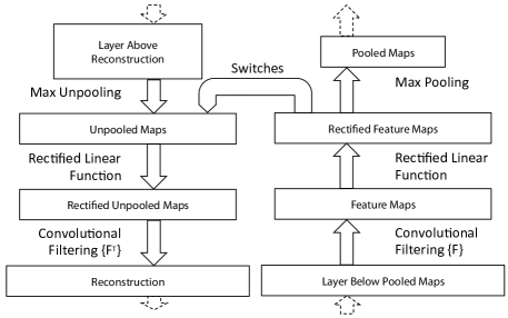
To examine a convnet, a deconvnet is attached to each of its layers, as illustrated in Fig. 1(top), providing a continuous path back to image pixels. To start, an input image is presented to the convnet and features computed throughout the layers. To examine a given convnet activation, we set all other activations in the layer to zero and pass the feature maps as input to the attached deconvnet layer. Then we successively (i) unpool, (ii) rectify and (iii) filter to reconstruct the activity in the layer beneath that gave rise to the chosen activation. This is then repeated until input pixel space is reached.

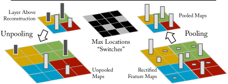
Unpooling: In the convnet, the max pooling operation is non-invertible, however we can obtain an approximate inverse by recording the locations of the maxima within each pooling region in a set of switch variables. In the deconvnet, the unpooling operation uses these switches to place the reconstructions from the layer above into appropriate locations, preserving the structure of the stimulus. See Fig. 1(bottom) for an illustration of the procedure.

Rectification: The convnet uses relu non-linearities, which rectify the feature maps thus ensuring the feature maps are always positive. To obtain valid feature reconstructions at each layer (which also should be positive), we pass the reconstructed signal through a relu non-linearity.

Filtering: The convnet uses learned filters to convolve the feature maps from the previous layer. To invert this, the deconvnet uses transposed versions of the same filters, but applied to the rectified maps, not the output of the layer beneath. In practice this means flipping each filter vertically and horizontally.

Projecting down from higher layers uses the switch settings generated by the max pooling in the convnet on the way up. As these switch settings are peculiar to a given input image, the reconstruction obtained from a single activation thus resembles a small piece of the original input image, with structures weighted according to their contribution toward to the feature activation. Since the model is trained discriminatively, they implicitly show which parts of the input image are discriminative. Note that these projections are not samples from the model, since there is no generative process involved.

Figure 1: Top: A deconvnet layer (left) attached to a convnet layer (right). The deconvnet will reconstruct an approximate version of the convnet features from the layer beneath. Bottom: An illustration of the unpooling operation in the deconvnet, using switches which record the location of the local max in each pooling region (colored zones) during pooling in the convnet.

3 Training Details

We now describe the large convnet model that will be visualized in Section 4. The architecture, shown in Fig. 3, is similar to that used by (Krizhevsky et al., 2012) for ImageNet classification. One difference is that the sparse connections used in Krizhevsky’s layers 3,4,5 (due to the model being split across 2 GPUs) are replaced with dense connections in our model. Other important differences relating to layers 1 and 2 were made following inspection of the visualizations in Fig. 6, as described in Section 4.1.

The model was trained on the ImageNet 2012 training set (1.3 million images, spread over 1000 different classes). Each RGB image was preprocessed by resizing the smallest dimension to 256, cropping the center 256x256 region, subtracting the per-pixel mean (across all images) and then using 10 different sub-crops of size 224x224 (corners $+$ center with(out) horizontal flips). Stochastic gradient descent with a mini-batch size of 128 was used to update the parameters, starting with a learning rate of $10^{-2}$, in conjunction with a momentum term of $0.9$. We anneal the learning rate throughout training manually when the validation error plateaus. Dropout (Hinton et al., 2012) is used in the fully connected layers (6 and 7) with a rate of 0.5. All weights are initialized to $10^{-2}$ and biases are set to 0.

Visualization of the first layer filters during training reveals that a few of them dominate, as shown in Fig. 6(a). To combat this, we renormalize each filter in the convolutional layers whose RMS value exceeds a fixed radius of $10^{-1}$ to this fixed radius. This is crucial, especially in the first layer of the model, where the input images are roughly in the [-128,128] range. As in (Krizhevsky et al., 2012), we produce multiple different crops and flips of each training example to boost training set size. We stopped training after 70 epochs, which took around 12 days on a single GTX580 GPU, using an implementation based on (Krizhevsky et al., 2012).

4 Convnet Visualization

Using the model described in Section 3, we now use the deconvnet to visualize the feature activations on the ImageNet validation set.

Feature Visualization: Fig. 2 shows feature visualizations from our model once training is complete. However, instead of showing the single strongest activation for a given feature map, we show the top 9 activations. Projecting each separately down to pixel space reveals the different structures that excite a given feature map, hence showing its invariance to input deformations. Alongside these visualizations we show the corresponding image patches. These have greater variation than visualizations as the latter solely focus on the discriminant structure within each patch. For example, in layer 5, row 1, col 2, the patches appear to have little in common, but the visualizations reveal that this particular feature map focuses on the grass in the background, not the foreground objects.

Figure 2: Visualization of features in a fully trained model. For layers 2-5 we show the top 9 activations in a random subset of feature maps across the validation data, projected down to pixel space using our deconvolutional network approach. Our reconstructions are not samples from the model: they are reconstructed patterns from the validation set that cause high activations in a given feature map. For each feature map we also show the corresponding image patches. Note: (i) the the strong grouping within each feature map, (ii) greater invariance at higher layers and (iii) exaggeration of discriminative parts of the image, e.g. eyes and noses of dogs (layer 4, row 1, cols 1). Best viewed in electronic form.

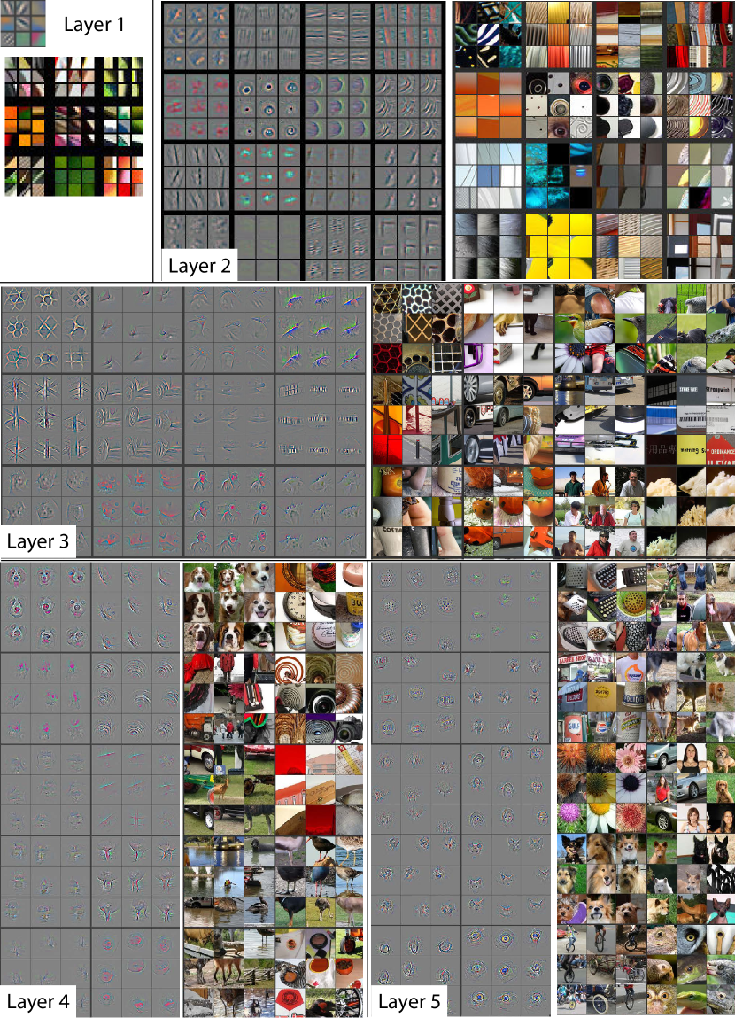
The projections from each layer show the hierarchical nature of the features in the network. Layer 2 responds to corners and other edge/color conjunctions. Layer 3 has more complex invariances, capturing similar textures (e.g. mesh patterns (Row 1, Col 1); text (R2,C4)). Layer 4 shows significant variation, but is more class-specific: dog faces (R1,C1); bird’s legs (R4,C2). Layer 5 shows entire objects with significant pose variation, e.g. keyboards (R1,C11) and dogs (R4).

Figure 3: Architecture of our 8 layer convnet model. A 224 by 224 crop of an image (with 3 color planes) is presented as the input. This is convolved with 96 different 1st layer filters (red), each of size 7 by 7, using a stride of 2 in both x and y. The resulting feature maps are then: (i) passed through a rectified linear function (not shown), (ii) pooled (max within 3x3 regions, using stride 2) and (iii) contrast normalized across feature maps to give 96 different 55 by 55 element feature maps. Similar operations are repeated in layers 2,3,4,5. The last two layers are fully connected, taking features from the top convolutional layer as input in vector form (6 $\cdot$ 6 $\cdot$ 256 = 9216 dimensions). The final layer is a $C$-way softmax function, $C$ being the number of classes. All filters and feature maps are square in shape.

Feature Evolution during Training: Fig. 4 visualizes the progression during training of the strongest activation (across all training examples) within a given feature map projected back to pixel space. Sudden jumps in appearance result from a change in the image from which the strongest activation originates. The lower layers of the model can be seen to converge within a few epochs. However, the upper layers only develop develop after a considerable number of epochs (40-50), demonstrating the need to let the models train until fully converged.

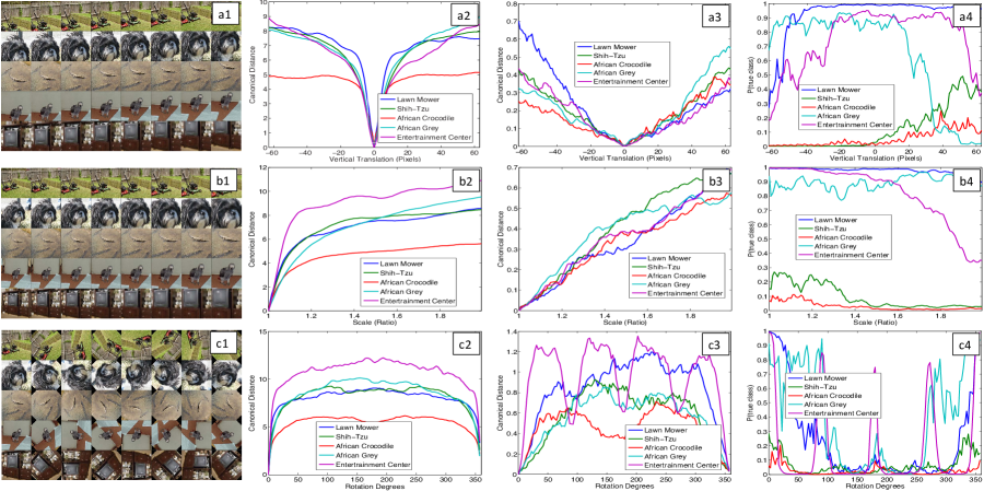
Feature Invariance: Fig. 5 shows 5 sample images being translated, rotated and scaled by varying degrees while looking at the changes in the feature vectors from the top and bottom layers of the model, relative to the untransformed feature. Small transformations have a dramatic effect in the first layer of the model, but a lesser impact at the top feature layer, being quasi-linear for translation & scaling. The network output is stable to translations and scalings. In general, the output is not invariant to rotation, except for object with rotational symmetry (e.g. entertainment center).

Figure 4: Evolution of a randomly chosen subset of model features through training. Each layer’s features are displayed in a different block. Within each block, we show a randomly chosen subset of features at epochs [1,2,5,10,20,30,40,64]. The visualization shows the strongest activation (across all training examples) for a given feature map, projected down to pixel space using our deconvnet approach. Color contrast is artificially enhanced and the figure is best viewed in electronic form.

Figure 5: Analysis of vertical translation, scale, and rotation invariance within the model (rows a-c respectively). Col 1: 5 example images undergoing the transformations. Col 2 & 3: Euclidean distance between feature vectors from the original and transformed images in layers 1 and 7 respectively. Col 4: the probability of the true label for each image, as the image is transformed.

4.1 Architecture Selection

While visualization of a trained model gives insight into its operation, it can also assist with selecting good architectures in the first place. By visualizing the first and second layers of Krizhevsky et al. ’s architecture (Fig. 6(b) & (d)), various problems are apparent. The first layer filters are a mix of extremely high and low frequency information, with little coverage of the mid frequencies. Additionally, the 2nd layer visualization shows aliasing artifacts caused by the large stride 4 used in the 1st layer convolutions. To remedy these problems, we (i) reduced the 1st layer filter size from 11x11 to 7x7 and (ii) made the stride of the convolution 2, rather than 4. This new architecture retains much more information in the 1st and 2nd layer features, as shown in Fig. 6(c) & (e). More importantly, it also improves the classification performance as shown in Section 2.

Figure 6: (a): 1st layer features without feature scale clipping. Note that one feature dominates. (b): 1st layer features from (Krizhevsky et al., 2012). (c): Our 1st layer features. The smaller stride (2 vs 4) and filter size (7x7 vs 11x11) results in more distinctive features and fewer “dead” features. (d): Visualizations of 2nd layer features from (Krizhevsky et al., 2012). (e): Visualizations of our 2nd layer features. These are cleaner, with no aliasing artifacts that are visible in (d).

4.2 Occlusion Sensitivity

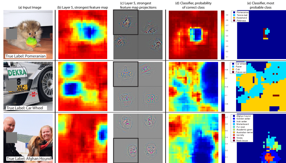
With image classification approaches, a natural question is if the model is truly identifying the location of the object in the image, or just using the surrounding context. Fig. 7 attempts to answer this question by systematically occluding different portions of the input image with a grey square, and monitoring the output of the classifier. The examples clearly show the model is localizing the objects within the scene, as the probability of the correct class drops significantly when the object is occluded. Fig. 7 also shows visualizations from the strongest feature map of the top convolution layer, in addition to activity in this map (summed over spatial locations) as a function of occluder position. When the occluder covers the image region that appears in the visualization, we see a strong drop in activity in the feature map. This shows that the visualization genuinely corresponds to the image structure that stimulates that feature map, hence validating the other visualizations shown in Fig. 4 and Fig. 2.

Figure 7: Three test examples where we systematically cover up different portions of the scene with a gray square (1st column) and see how the top (layer 5) feature maps ((b) & (c)) and classifier output ((d) & (e)) changes. (b): for each position of the gray scale, we record the total activation in one layer 5 feature map (the one with the strongest response in the unoccluded image). (c): a visualization of this feature map projected down into the input image (black square), along with visualizations of this map from other images. The first row example shows the strongest feature to be the dog’s face. When this is covered-up the activity in the feature map decreases (blue area in (b)). (d): a map of correct class probability, as a function of the position of the gray square. E.g. when the dog’s face is obscured, the probability for “pomeranian” drops significantly. (e): the most probable label as a function of occluder position. E.g. in the 1st row, for most locations it is “pomeranian”, but if the dog’s face is obscured but not the ball, then it predicts “tennis ball”. In the 2nd example, text on the car is the strongest feature in layer 5, but the classifier is most sensitive to the wheel. The 3rd example contains multiple objects. The strongest feature in layer 5 picks out the faces, but the classifier is sensitive to the dog (blue region in (d)), since it uses multiple feature maps.

4.3 Correspondence Analysis

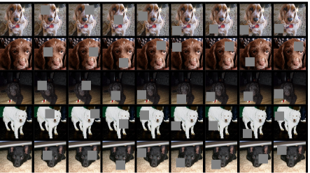
Deep models differ from many existing recognition approaches in that there is no explicit mechanism for establishing correspondence between specific object parts in different images (e.g. faces have a particular spatial configuration of the eyes and nose). However, an intriguing possibility is that deep models might be implicitly computing them. To explore this, we take 5 randomly drawn dog images with frontal pose and systematically mask out the same part of the face in each image (e.g. all left eyes, see Fig. 8). For each image $i$, we then compute: $\epsilon^{l}_{i}=x^{l}_{i}-\tilde{x}^{l}_{i}$, where $x^{l}_{i}$ and $\tilde{x}^{l}_{i}$ are the feature vectors at layer $l$ for the original and occluded images respectively. We then measure the consistency of this difference vector $\epsilon$ between all related image pairs $(i,j)$: $\Delta_{l}=\sum_{i,j=1,i\neq j}^{5}\mathcal{H}(\text{sign}(\epsilon^{l}_{i}),\text{sign}(\epsilon^{l}_{j}))$, where $\mathcal{H}$ is Hamming distance. A lower value indicates greater consistency in the change resulting from the masking operation, hence tighter correspondence between the same object parts in different images (i.e. blocking the left eye changes the feature representation in a consistent way). In Table 1 we compare the $\Delta$ score for three parts of the face (left eye, right eye and nose) to random parts of the object, using features from layer $l=5$ and $l=7$. The lower score for these parts, relative to random object regions, for the layer $5$ features show the model does establish some degree of correspondence.

Figure 8: Images used for correspondence experiments. Col 1: Original image. Col 2,3,4: Occlusion of the right eye, left eye, and nose respectively. Other columns show examples of random occlusions.

	Mean Feature	Mean Feature
	Sign Change	Sign Change
Occlusion Location	Layer 5	Layer 7
Right Eye	$0.067\pm 0.007$	$0.069\pm 0.015$
Left Eye	$0.069\pm 0.007$	$0.068\pm 0.013$
Nose	$0.079\pm 0.017$	$0.069\pm 0.011$
Random	$0.107\pm 0.017$	$0.073\pm 0.014$

Table 1: Measure of correspondence for different object parts in 5 different dog images. The lower scores for the eyes and nose (compared to random object parts) show the model implicitly establishing some form of correspondence of parts at layer 5 in the model. At layer 7, the scores are more similar, perhaps due to upper layers trying to discriminate between the different breeds of dog.

5 Experiments

5.1 ImageNet 2012

This dataset consists of 1.3M/50k/100k training/validation/test examples, spread over 1000 categories. Table 2 shows our results on this dataset.

Using the exact architecture specified in (Krizhevsky et al., 2012), we attempt to replicate their result on the validation set. We achieve an error rate within $0.1\%$ of their reported value on the ImageNet 2012 validation set.

Next we analyze the performance of our model with the architectural changes outlined in Section 4.1 ($7\times 7$ filters in layer 1 and stride $2$ convolutions in layers 1 & 2). This model, shown in Fig. 3, significantly outperforms the architecture of (Krizhevsky et al., 2012), beating their single model result by $1.7\%$ (test top-5). When we combine multiple models, we obtain a test error of ${\bf 14.8\%}$, the best published performance on this dataset (despite only using the 2012 training set). We note that this error is almost half that of the top non-convnet entry in the ImageNet 2012 classification challenge, which obtained $26.2\%$ error (Gunji et al., 2012).

	Val	Val	Test
Error %	Top-1	Top-5	Top-5
(Gunji et al., 2012)	-	-	$26.2$
(Krizhevsky et al., 2012), 1 convnet	$40.7$	$18.2$	$--$
(Krizhevsky et al., 2012), 5 convnets	$38.1$	$16.4$	$16.4$
(Krizhevsky et al., 2012)∗, 1 convnets	$39.0$	$16.6$	$--$
(Krizhevsky et al., 2012)∗, 7 convnets	$36.7$	$15.4$	$15.3$
Our replication of
(Krizhevsky et al., 2012), 1 convnet	$40.5$	$18.1$	$--$
1 convnet as per Fig. 3	$38.4$	$16.5$	$--$
5 convnets as per Fig. 3 – (a)	$36.7$	$15.3$	$15.3$
1 convnet as per Fig. 3 but with
layers 3,4,5: 512,1024,512 maps – (b)	$37.5$	$16.0$	$16.1$
6 convnets, (a) & (b) combined	$\bf{36.0}$	$\bf{14.7}$	$\bf{14.8}$

Table 2: ImageNet 2012 classification error rates. The $*$ indicates models that were trained on both ImageNet 2011 and 2012 training sets.

Varying ImageNet Model Sizes: In Table 3, we first explore the architecture of (Krizhevsky et al., 2012) by adjusting the size of layers, or removing them entirely. In each case, the model is trained from scratch with the revised architecture. Removing the fully connected layers (6,7) only gives a slight increase in error. This is surprising, given that they contain the majority of model parameters. Removing two of the middle convolutional layers also makes a relatively small different to the error rate. However, removing both the middle convolution layers and the fully connected layers yields a model with only 4 layers whose performance is dramatically worse. This would suggest that the overall depth of the model is important for obtaining good performance. In Table 3, we modify our model, shown in Fig. 3. Changing the size of the fully connected layers makes little difference to performance (same for model of (Krizhevsky et al., 2012)). However, increasing the size of the middle convolution layers goes give a useful gain in performance. But increasing these, while also enlarging the fully connected layers results in over-fitting.

	Train	Val	Val
Error %	Top-1	Top-1	Top-5
Our replication of
(Krizhevsky et al., 2012), 1 convnet	$35.1$	$40.5$	$18.1$
Removed layers 3,4	$41.8$	$45.4$	$22.1$
Removed layer 7	$27.4$	$40.0$	$18.4$
Removed layers 6,7	$27.4$	$44.8$	$22.4$
Removed layer 3,4,6,7	$71.1$	$71.3$	$50.1$
Adjust layers 6,7: 2048 units	$40.3$	$41.7$	$18.8$
Adjust layers 6,7: 8192 units	$26.8$	$40.0$	$18.1$
Our Model (as per Fig. 3)	$33.1$	$38.4$	$16.5$
Adjust layers 6,7: 2048 units	$38.2$	$40.2$	$17.6$
Adjust layers 6,7: 8192 units	$22.0$	$38.8$	$17.0$
Adjust layers 3,4,5: 512,1024,512 maps	$18.8$	$\bf{37.5}$	$\bf{16.0}$
Adjust layers 6,7: 8192 units and
Layers 3,4,5: 512,1024,512 maps	$\bf{10.0}$	$38.3$	$16.9$

Table 3: ImageNet 2012 classification error rates with various architectural changes to the model of (Krizhevsky et al., 2012) and our model (see Fig. 3).

5.2 Feature Generalization

The experiments above show the importance of the convolutional part of our ImageNet model in obtaining state-of-the-art performance. This is supported by the visualizations of Fig. 2 which show the complex invariances learned in the convolutional layers. We now explore the ability of these feature extraction layers to generalize to other datasets, namely Caltech-101 (Fei-fei et al., 2006), Caltech-256 (Griffin et al., 2006) and PASCAL VOC 2012. To do this, we keep layers 1-7 of our ImageNet-trained model fixed and train a new softmax classifier on top (for the appropriate number of classes) using the training images of the new dataset. Since the softmax contains relatively few parameters, it can be trained quickly from a relatively small number of examples, as is the case for certain datasets.

The classifiers used by our model (a softmax) and other approaches (typically a linear SVM) are of similar complexity, thus the experiments compare our feature representation, learned from ImageNet, with the hand-crafted features used by other methods. It is important to note that both our feature representation and the hand-crafted features are designed using images beyond the Caltech and PASCAL training sets. For example, the hyper-parameters in HOG descriptors were determined through systematic experiments on a pedestrian dataset (Dalal & Triggs, 2005). We also try a second strategy of training a model from scratch, i.e. resetting layers 1-7 to random values and train them, as well as the softmax, on the training images of the dataset.

One complication is that some of the Caltech datasets have some images that are also in the ImageNet training data. Using normalized correlation, we identified these few “overlap” images and removed them from our Imagenet training set and then retrained our Imagenet models, so avoiding the possibility of train/test contamination.

Caltech-101: We follow the procedure of (Fei-fei et al., 2006) and randomly select 15 or 30 images per class for training and test on up to 50 images per class reporting the average of the per-class accuracies in Table 4, using 5 train/test folds. Training took 17 minutes for 30 images/class. The pre-trained model beats the best reported result for 30 images/class from (Bo et al., 2013) by 2.2%. The convnet model trained from scratch however does terribly, only achieving 46.5%.

	Acc %	Acc %
# Train	15/class	30/class
(Bo et al., 2013)	$-$	$81.4\pm 0.33$
(Jianchao et al., 2009)	$73.2$	$84.3$
Non-pretrained convnet	$22.8\pm 1.5$	$46.5\pm 1.7$
ImageNet-pretrained convnet	$\bf{83.8\pm 0.5}$	$\bf{86.5\pm 0.5}$

Table 4: Caltech-101 classification accuracy for our convnet models, against two leading alternate approaches.

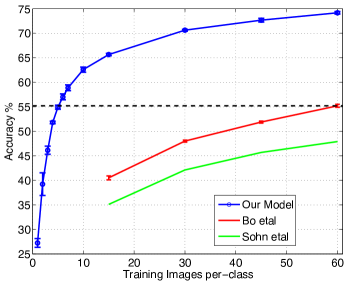
Caltech-256: We follow the procedure of (Griffin et al., 2006), selecting 15, 30, 45, or 60 training images per class, reporting the average of the per-class accuracies in Table 5. Our ImageNet-pretrained model beats the current state-of-the-art results obtained by Bo et al. (Bo et al., 2013) by a significant margin: 74.2% vs 55.2% for 60 training images/class. However, as with Caltech-101, the model trained from scratch does poorly. In Fig. 9, we explore the “one-shot learning” (Fei-fei et al., 2006) regime. With our pre-trained model, just 6 Caltech-256 training images are needed to beat the leading method using 10 times as many images. This shows the power of the ImageNet feature extractor.

	Acc %	Acc %	Acc %	Acc %
# Train	15/class	30/class	45/class	60/class
(Sohn et al., 2011)	$35.1$	$42.1$	$45.7$	$47.9$
(Bo et al., 2013)	$40.5\pm 0.4$	$48.0\pm 0.2$	$51.9\pm 0.2$	$55.2\pm 0.3$
Non-pretr.	$9.0\pm 1.4$	$22.5\pm 0.7$	$31.2\pm 0.5$	$38.8\pm 1.4$
ImageNet-pretr.	$\bf{65.7\pm 0.2}$	$\bf{70.6\pm 0.2}$	$\bf{72.7\pm 0.4}$	$\bf{74.2\pm 0.3}$

Table 5: Caltech 256 classification accuracies.

Figure 9: Caltech-256 classification performance as the number of training images per class is varied. Using only 6 training examples per class with our pre-trained feature extractor, we surpass best reported result by (Bo et al., 2013).

PASCAL 2012: We used the standard training and validation images to train a 20-way softmax on top of the ImageNet-pretrained convnet. This is not ideal, as PASCAL images can contain multiple objects and our model just provides a single exclusive prediction for each image. Table 6 shows the results on the test set. The PASCAL and ImageNet images are quite different in nature, the former being full scenes unlike the latter. This may explain our mean performance being $3.2\%$ lower than the leading (Yan et al., 2012) result, however we do beat them on 5 classes, sometimes by large margins.

Acc %	[A]	[B]	Ours	Acc %	[A]	[B]	Ours
Airplane	92.0	97.3	96.0	Dining tab	63.2	77.8	67.7
Bicycle	74.2	84.2	77.1	Dog	68.9	83.0	87.8
Bird	73.0	80.8	88.4	Horse	78.2	87.5	86.0
Boat	77.5	85.3	85.5	Motorbike	81.0	90.1	85.1
Bottle	54.3	60.8	55.8	Person	91.6	95.0	90.9
Bus	85.2	89.9	85.8	Potted pl	55.9	57.8	52.2
Car	81.9	86.8	78.6	Sheep	69.4	79.2	83.6
Cat	76.4	89.3	91.2	Sofa	65.4	73.4	61.1
Chair	65.2	75.4	65.0	Train	86.7	94.5	91.8
Cow	63.2	77.8	74.4	Tv	77.4	80.7	76.1
Mean	74.3	82.2	79.0	# won	0	15	5

Table 6: PASCAL 2012 classification results, comparing our Imagenet-pretrained convnet against the leading two methods ([A]= (Sande et al., 2012) and [B] = (Yan et al., 2012)).

5.3 Feature Analysis

We explore how discriminative the features in each layer of our Imagenet-pretrained model are. We do this by varying the number of layers retained from the ImageNet model and place either a linear SVM or softmax classifier on top. Table 7 shows results on Caltech-101 and Caltech-256. For both datasets, a steady improvement can be seen as we ascend the model, with best results being obtained by using all layers. This supports the premise that as the feature hierarchies become deeper, they learn increasingly powerful features.

	Cal-101	Cal-256
	(30/class)	(60/class)
SVM (1)	$44.8\pm 0.7$	$24.6\pm 0.4$
SVM (2)	$66.2\pm 0.5$	$39.6\pm 0.3$
SVM (3)	$72.3\pm 0.4$	$46.0\pm 0.3$
SVM (4)	$76.6\pm 0.4$	$51.3\pm 0.1$
SVM (5)	$\bf{86.2\pm 0.8}$	$65.6\pm 0.3$
SVM (7)	$\bf{85.5\pm 0.4}$	$\bf{71.7\pm 0.2}$
Softmax (5)	$82.9\pm 0.4$	$65.7\pm 0.5$
Softmax (7)	$\bf{85.4\pm 0.4}$	$\bf{72.6\pm 0.1}$

Table 7: Analysis of the discriminative information contained in each layer of feature maps within our ImageNet-pretrained convnet. We train either a linear SVM or softmax on features from different layers (as indicated in brackets) from the convnet. Higher layers generally produce more discriminative features.

6 Discussion

We explored large convolutional neural network models, trained for image classification, in a number ways. First, we presented a novel way to visualize the activity within the model. This reveals the features to be far from random, uninterpretable patterns. Rather, they show many intuitively desirable properties such as compositionality, increasing invariance and class discrimination as we ascend the layers. We also showed how these visualization can be used to debug problems with the model to obtain better results, for example improving on Krizhevsky et al. ’s (Krizhevsky et al., 2012) impressive ImageNet 2012 result. We then demonstrated through a series of occlusion experiments that the model, while trained for classification, is highly sensitive to local structure in the image and is not just using broad scene context. An ablation study on the model revealed that having a minimum depth to the network, rather than any individual section, is vital to the model’s performance.

Finally, we showed how the ImageNet trained model can generalize well to other datasets. For Caltech-101 and Caltech-256, the datasets are similar enough that we can beat the best reported results, in the latter case by a significant margin. This result brings into question to utility of benchmarks with small (i.e. $<10^{4}$) training sets. Our convnet model generalized less well to the PASCAL data, perhaps suffering from dataset bias (Torralba & Efros, 2011), although it was still within $3.2\%$ of the best reported result, despite no tuning for the task. For example, our performance might improve if a different loss function was used that permitted multiple objects per image. This would naturally enable the networks to tackle the object detection as well.

References

- Bengio et al. (2007) Bengio, Y., Lamblin, P., Popovici, D., and Larochelle, H. Greedy layer-wise training of deep networks. In NIPS, pp. 153–160, 2007.
- Berkes & Wiskott (2006) Berkes, P. and Wiskott, L. On the analysis and interpretation of inhomogeneous quadratic forms as receptive fields. Neural Computation, 2006.
- Bo et al. (2013) Bo, L., Ren, X., and Fox, D. Multipath sparse coding using hierarchical matching pursuit. In CVPR, 2013.
- Ciresan et al. (2012) Ciresan, D. C., Meier, J., and Schmidhuber, J. Multi-column deep neural networks for image classification. In CVPR, 2012.
- Dalal & Triggs (2005) Dalal, N. and Triggs, B. Histograms of oriented gradients for pedestrian detection. In CVPR, 2005.
- Donahue et al. (2013) Donahue, J., Jia, Y., Vinyals, O., Hoffman, J., Zhang, N., Tzeng, E., and Darrell, T. DeCAF: A deep convolutional activation feature for generic visual recognition. In arXiv:1310.1531, 2013.
- Erhan et al. (2009) Erhan, D., Bengio, Y., Courville, A., and Vincent, P. Visualizing higher-layer features of a deep network. In Technical report, University of Montreal, 2009.
- Fei-fei et al. (2006) Fei-fei, L., Fergus, R., and Perona, P. One-shot learning of object categories. IEEE Trans. PAMI, 2006.
- Griffin et al. (2006) Griffin, G., Holub, A., and Perona, P. The caltech 256. In Caltech Technical Report, 2006.
- Gunji et al. (2012) Gunji, N., Higuchi, T., Yasumoto, K., Muraoka, H., Ushiku, Y., Harada, T., and Kuniyoshi, Y. Classification entry. In Imagenet Competition, 2012.
- Hinton et al. (2006) Hinton, G. E., Osindero, S., and The, Y. A fast learning algorithm for deep belief nets. Neural Computation, 18:1527–1554, 2006.
- Hinton et al. (2012) Hinton, G.E., Srivastave, N., Krizhevsky, A., Sutskever, I., and Salakhutdinov, R. R. Improving neural networks by preventing co-adaptation of feature detectors. arXiv:1207.0580, 2012.
- Jarrett et al. (2009) Jarrett, K., Kavukcuoglu, K., Ranzato, M., and LeCun, Y. What is the best multi-stage architecture for object recognition? In ICCV, 2009.
- Jianchao et al. (2009) Jianchao, Y., Kai, Y., Yihong, G., and Thomas, H. Linear spatial pyramid matching using sparse coding for image classification. In CVPR, 2009.
- Krizhevsky et al. (2012) Krizhevsky, A., Sutskever, I., and Hinton, G.E. Imagenet classification with deep convolutional neural networks. In NIPS, 2012.
- Le et al. (2010) Le, Q. V., Ngiam, J., Chen, Z., Chia, D., Koh, P., and Ng, A. Y. Tiled convolutional neural networks. In NIPS, 2010.
- LeCun et al. (1989) LeCun, Y., Boser, B., Denker, J. S., Henderson, D., Howard, R. E., Hubbard, W., and Jackel, L. D. Backpropagation applied to handwritten zip code recognition. Neural Comput., 1(4):541–551, 1989.
- Sande et al. (2012) Sande, K., Uijlings, J., Snoek, C., and Smeulders, A. Hybrid coding for selective search. In PASCAL VOC Classification Challenge 2012, 2012.
- Sohn et al. (2011) Sohn, K., Jung, D., Lee, H., and Hero III, A. Efficient learning of sparse, distributed, convolutional feature representations for object recognition. In ICCV, 2011.
- Torralba & Efros (2011) Torralba, A. and Efros, A. A. Unbiased look at dataset bias. In CVPR, 2011.
- Vincent et al. (2008) Vincent, P., Larochelle, H., Bengio, Y., and Manzagol, P. A. Extracting and composing robust features with denoising autoencoders. In ICML, pp. 1096–1103, 2008.
- Yan et al. (2012) Yan, S., Dong, J., Chen, Q., Song, Z., Pan, Y., Xia, W., Huang, Z., Hua, Y., and Shen, S. Generalized hierarchical matching for sub-category aware object classification. In PASCAL VOC Classification Challenge 2012, 2012.
- Zeiler et al. (2011) Zeiler, M., Taylor, G., and Fergus, R. Adaptive deconvolutional networks for mid and high level feature learning. In ICCV, 2011.