Towards a continuum model for particle-induced velocity fluctuations in suspension flow through a stenosed geometry

Abstract

Non-particulate continuum descriptions allow for computationally efficient modeling of suspension flows at scales that are inaccessible to more detailed particulate approaches. It is well known that the presence of particles influences the effective viscosity of a suspension and that this effect has thus to be accounted for in macroscopic continuum models. The present paper aims at developing a non-particulate model that reproduces not only the rheology but also the cell-induced velocity fluctuations, responsible for enhanced diffusivity. The results are obtained from a coarse-grained blood model based on the lattice Boltzmann method. The benchmark system comprises a flow between two parallel plates with one of them featuring a smooth obstacle imitating a stenosis. Appropriate boundary conditions are developed for the particulate model to generate equilibrated cell configurations mimicking an infinite channel in front of the stenosis. The averaged flow field in the bulk of the channel can be described well by a non-particulate simulation with a matched viscosity. We show that our proposed phenomenological model is capable to reproduce many features of the velocity fluctuations.

I Introduction

The presence of particles in a flowing suspension causes macroscopically relevant effects via small disturbances of the local velocity of the suspending medium even for laminar homogeneous flows. This effect can augment the transport through the suspension zydney88 ; ishikawa08 . An important example is blood which is a suspension mostly consisting of red blood cells (RBCs) in blood plasma. Of special interest for medical applications is the transport of plasma molecules which due to their dimensions can be assumed to follow the streamlines of the flow and which play a crucial role in blood clotting phenomena. While advances in the development of coarse-grained blood models have been made, simulations of realistic vessel geometries at particulate resolution are still computationally expensive janoschek10 ; melchionna11 . Therefore, continuous descriptions of blood are applied frequently to study flows at large scales, compared to single cells, eventually supported by a continuous description of the effective transport of cellular and molecular blood constituents boyd05 ; mikhal12 ; sorensen99 .

The present work aims instead at developing a continuous description of the fluid velocity fluctuations and its comparison with large-scale particulate simulations in an infinite channel with a single constriction. A similar geometry is modeled, for example, in Ref. ishikawa07 . Defining appropriate boundary conditions for the inlet and outlet is not trivial in the case of suspensions. Section II briefly introduces the coarse-grained particulate blood model janoschek10 employed here. Section III contains a description of the required boundary conditions in a parallel implementation. Section IV deals with the reconstruction of the flow field and of the plasma velocity fluctuations in a non-particulate simulation. Conclusions are drawn in Section V.

II Simulation method

In an earlier work, a simplified particulate blood model was developed janoschek10 . RBCs are described as oblate spheroids coupled to a lattice Boltzmann (LB) method succi01 that accounts for the blood plasma. One lattice spacing resembles $0.667\,\upmu\mathrm{m}$, one LB time step $6.80\times 10^{-8}\,\mathrm{s}$. All parameters are chosen as in Ref. janoschek10 . A pair of mutual forces

$$\mathbf{F}^{+}=2n_{r}^{\text{eq}}(\bar{\rho},\mathbf{u}{=}\mathbf{0})\mathbf{c}_{r}\text{\quad and\quad}\mathbf{F}^{-}=-\mathbf{F}^{+}$$ (1)

at lattice links connecting two cells corrects for the lack of fluid pressure at cell-cell interfaces. $n_{r}^{\mathrm{eq}}(\bar{\rho},\mathbf{u})$ stands for the LB equilibrium distribution function for density $\bar{\rho}$ and velocity $\mathbf{u}$ of the fluid and $\mathbf{c}_{r}$ for the respective lattice vector. The present simulations are the first application of this model to a situation where—due to the drop of the pressure $P$ induced by the stenosis—the fluid density $\rho\sim P$ varies macroscopically across a system with many cells. Under these conditions, the global average $\bar{\rho}$ in Eq. (1) has to be replaced by a local average $(\bar{\rho}_{i}+\bar{\rho}_{j})/2$ between cells $i$ and $j$ to prevent artificial attraction or repulsion. $\bar{\rho}_{\alpha}$ is an average over all fluid sites at the surface of cell $\alpha$. Further, $\bar{\rho}_{i}$ is used as the new fluid density wherever a lattice site occupied by cell $i$ before is freed and to compute Eq. (1) at direct cell-wall links. Sometimes a slight mass drift is observed whereas a constant density $\bar{\rho}$ makes significant spatial variations of $\rho$ impossible in the presence of many cells. Therefore, all densities are rescaled periodically to keep the global average density constant. In the simulations below, the required rescaling factor differs by less than $10^{-3}$ from unity if rescaling is performed every $1000$ time steps.

Since Eq. (1) does not account for dissipation at cell-cell contacts, a further adaption is made: the force on cell $i$ resulting from a link to a site of cell $j$ is computed not from Eq. (1) but assuming fluid at distribution $n_{r}^{\mathrm{eq}}((\bar{\rho}_{i}+\bar{\rho}_{j})/2,\mathbf{u}_{j})$ at the site belonging to $j$. $\mathbf{u}_{j}$ is $j$’s local velocity half-way along the link. The resulting forces on two cells remain opposite but equal up to first order in velocity. Similarly, for cell-wall links, a fluid distribution $n_{r}^{\mathrm{eq}}(\bar{\rho}_{i},\mathbf{0})$ is assumed at the wall site. At a cell volume fraction of $\Phi\approx 0.43$, the new contact rule leads to an enhancement of the relative suspension viscosity $\mu_{\mathrm{r}}$ by $0.5$ to $1$ or about $10\,\%$ to $30\,\%$ for shear rates $50\,\mathrm{s}^{-1}<\dot{\gamma}<2\times 10^{3}\,\mathrm{s}^{-1}$. Accurate sub-lattice corrections for the hydrodynamic interactions of rigid spheroidal particles near contact have been presented recently janoschek13 .

III Periodic inflow boundary conditions

The transition length that a suspension needs to flow through a channel until a macroscopically stable state is achieved is known to be particularly large because of the time required for the particles to re-distribute in response to the laterally inhomogeneous flow nott94 . Since an appropriately long simulation volume is computationally too expensive, one could close the geometry in the flow direction with periodic boundary conditions and simulate for times long enough that each cell and each volume of fluid passes the system several times. There is the concrete risk, however, that because of the same effect nott94 the suspension would retain a memory of the stenosis and the simulation would describe not the flow through a stenosed channel but, in fact, the flow through an infinite series of stenoses. Appropriate boundary conditions are required that provide the cell configurations expected for a long channel without stenosis. The configuration expected for a long channel, however, is not known a priori. A solution is to develop boundary conditions that allow to independently simulate a periodic sub-volume resembling an infinitely long channel while the resulting configurations are fed into the inlet of the volume that contains the stenosis. The cells leaving the stenosed sub-volume are then discarded.

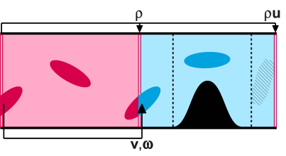
Figure 1: Schematic outline of the boundary conditions: fluid density $\rho$ and mass flow $\rho\mathbf{u}$ are copied from the first lattice layer of the periodic sub-volume to the first and last layer of the non-periodic volume, respectively. Translational and rotational cell velocities $\mathbf{v}$ and $\boldsymbol{\omega}$ of original periodic cells are imposed on copies in the non-periodic inlet region. The dashed lines indicate the end of this region and the start of the outflow region where cells are replaced with fluid.

The full procedure is sketched in Fig. 1. Copies of model cells in the periodic sub-volume are generated as soon as they approach the periodic boundary. While the copied cells are entering the non-periodic volume, their motion is still prescribed by the motion of the original cells. Once the cells in the non-periodic sub-volume have reached a longitudinal position about one cell diameter away from the entrance layer, the connection to the original cells is dismissed and the copied cells interact with the fluid and the surrounding cells as free particles. Before a cell in the non-periodic sub-volume reaches the last lattice layer, the sites occupied by it are replaced with fluid initialized according to the local rigid body motion of the cell and the average fluid density $\bar{\rho}_{i}$. On-site boundary conditions hecht10 impose the density $\rho$ and the mass flow $\rho\mathbf{u}$ obtained for every site of the first lattice layer of the periodic sub-volume on the first and the last layer of the non-periodic sub-volume, respectively. If, in the case of the mass flow, the source position is occupied by a model cell, an estimate is made based on its rigid body motion and the average fluid density.

In a parallel implementation, additional communication in the longitudinal direction is required with respect to a conventional three-dimensional domain decomposition scheme with periodically closed topology. The necessary communication steps are sketched exemplarily for the case of a two-dimensional decomposition into $5\times 2$ computational domains in Fig. 2. First, two-way communication is needed to establish the link to close the first sub-volume of the system periodically. Second, the density and mass flow need to be transferred to the processes holding the first and the last lattice layer of the remaining non-periodic volume. Similarly, the cell velocities from the beginning of the periodic sub-volume have to be sent to the beginning of the non-periodic sub-volume. The last step might involve communication to more than one destination process if the end of the entrance region (drawn as dashed line in Fig. 2(b)) lies in another domain than the sub-volume interface.

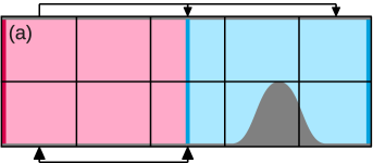
Figure 2: Communication requirements of the boundary conditions. Here an example is shown for the case of a decomposition into $5\times 2$ domains. Arrows indicate the direction along which information is sent. For (a) the plasma, the on-site boundary conditions require data from the periodic sub-volume which itself needs to be closed periodically. For (b) the cells, communication is required for the periodic boundaries as well and to prescribe the cell motion in the non-periodic entrance region.

The simulations are driven by a volume force $g_{z}$ in $z$-direction acting on every site within the periodic sub-volume. At sites occupied by a cell, the force is incorporated by the cell locally. $g_{z}$ is updated to a new value $g_{z}^{*}=g_{z}M_{z}^{*}/M_{z}$ at empirically determined time intervals in order to steer the mass flow $M_{z}$ towards an analytically estimated value $M_{z}^{*}$ for which the maximum flow velocity is close to $0.1$ in lattice units as a compromise between short simulation runs and the stability of the LB method. The resulting quotient of the maximum velocity $u_{\mathrm{max}}$ and the half-width of the opening of the constriction, an estimate for the average shear rate, amounts to ${\approx}5\times 10^{4}\,\mathrm{s}^{-1}$ in physical units. Though such shear rates, as the maximum flow velocity $u_{\mathrm{max}}\approx 1\,\mathrm{m}/\mathrm{s}$, under physiological conditions are not known for vessels with a diameter of only $85\,\upmu\mathrm{m}$ (see Ref. robertson08 ), the geometry can be understood as a very rough simplification of a real pathological stenosis and its partially curved geometry provides an interesting and well-defined test case. The Reynolds number is $\mathrm{Re}=\rho Hu_{\mathrm{max}}/(\mu_{\mathrm{r}}\mu_{0})\approx 9$ with the plasma viscosity $\mu_{0}$ when defined using the viscosity of the blood model for high shear rates as obtained in separate simulations.

IV Reconstruction of flow velocities and their fluctuations

The following study is performed for flow between two planar walls at a distance of $85\,\upmu\mathrm{m}$ in the $x$-direction and a length of $341\,\upmu\mathrm{m}$ in the $z$-direction. In the $y$-direction, the system is periodic with a depth of $85\,\upmu\mathrm{m}$. The lower wall carries a sinusoidal “stenosis” with a maximum height $H=42\,\upmu\mathrm{m}$. A mid-link bounce-back scheme ensures no-slip conditions at all walls. Fig. 3 shows an equilibrated snapshot of both the periodic and the non-periodic sub-volume. The volume fraction $\Phi=0.4$ leads to a total of ${\sim}10^{4}$ cells. After the constriction, a cell-free region develops in which recirculation is found. The flow velocity in $z$-direction $\langle u_{z}\rangle$ is reproduced in a continuous simulation without cells but with a viscosity matched to the high-shear viscosity of the blood model at $\Phi\approx 0.4$ which is achieved with an LB relaxation time of $\tau=2.15$. The averaging “$\langle\ldots\rangle$” is performed over equilibrated samples at different times and the periodic $y$-direction.

Figure 3: Snapshot of both sub-volumes after equilibration at a cell volume fraction of $\Phi=0.4$.

Fig. 4 compares the velocity fields $\langle u_{z}(z,x)\rangle$ from the particulate and $u_{z}^{=}(z,x)$ from the non-particulate simulation. Also the absolute and relative differences $u_{z}^{-}=u_{z}^{=}-\langle u_{z}\rangle$ and $|u_{z}^{-}/u_{z}^{+}|$ with $u_{z}^{+}=u_{z}^{=}+\langle u_{z}\rangle$ are plotted. Of course, the continuous model does not take into account the $\Phi$-induced deviations of $\mu_{\mathrm{r}}$ close to the solid walls. Thus, $u_{z}^{=}$ is too low in the otherwise cell-free boundary layers and consequently too high in the central region of the channel since the flow rate is kept constant. Still, the macroscopic features of the velocity field are reproduced relatively well. The relative difference is less than $10\,\%$ in the bulk region but higher than $50\,\%$ close to the walls and particularly in the recirculation zone which has two reasons: the low velocities there, which make small absolute differences more visible, and cell-depletion effects.

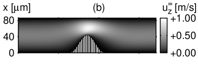
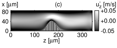
Figure 4: Comparison of (a) $\langle u_{z}\rangle$ at $\Phi=0.4$ and (b) $u_{z}^{=}$ at $\Phi=0$ with matched viscosity. (c) and (d) show the absolute and relative differences.

Fluctuations of the flow velocity $\mathbf{u}$ are quantified by the standard deviation

$$V=\operatorname{stdev}\,\mathbf{u}=\left[\sum_{\alpha=x,y,z}\left(\left\langle u_{\alpha}^{2}\right\rangle-\left\langle u_{\alpha}\right\rangle^{2}\right)\right]^{1/2}\text{ .}$$ (2)

The lateral profile $V(x)$ distant from the constriction is plotted in Fig. 5. $V$ reaches a maximum about one cell diameter away from the wall but does not increase further for shorter distances. Directly at the wall, no fluid is present and $V$ is zero. In the center of the channel, $V$ approximates a constant value of about one third of its maximum. In between, a roughly linear increase towards the wall is observed.

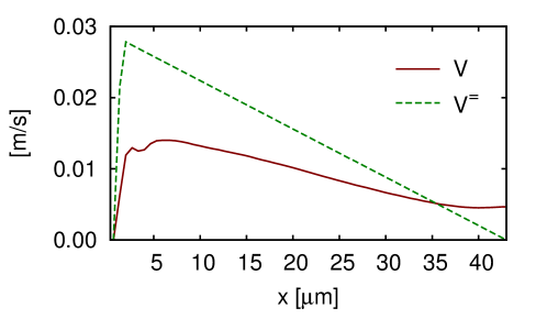
Figure 5: Lateral profile of the fluid velocity fluctuations $V$ without constriction. Shown is half of the channel cross section with the center at the right. Simulation data is compared to the dimensional estimate $V^{=}$ defined in Eq. (3) based on the shear rate in a continuous simulation.

Assuming that in the bulk of the suspension the time scale relevant for $V$ is the inverse undisturbed shear rate $\dot{\gamma}^{-1}$, which at scales much larger than single cells can easily be obtained from a non-particulate simulation, and that the relevant length scale must be of the order of the size of the cells, a dimensional estimate

$$V^{=}\simeq\dot{\gamma}R_{\parallel}$$ (3)

for $V$ induced by cells with shorter half-axes $R_{\parallel}$ is made. Also this estimate is plotted in Fig. 5, where the shear rate is obtained numerically from the continuous simulation as the derivative $\dot{\gamma}=\partial_{x}u_{z}^{=}$. For a Poiseuille flow, $\dot{\gamma}$ is a linear function of the lateral position and reaches its maximum at the wall. The decrease directly at the wall visible in Fig. 5 is caused by the absence of fluid at the wall itself and by artefacts of the numerical derivation. Eq. (3) reproduces the order of magnitude of the plasma velocity fluctuations correctly with an over-prediction of less than a factor two in the largest part of the plot. Also the linear dependence on the lateral position is observed for $V$ as well, at least in parts of the curve. The two regions where deviations from the linear shape are visible have a width of about one cell diameter and can indeed be attributed to cell effects: since cells cannot pass the vessel wall, the cell concentration immediately near to the wall is reduced and the motion of cells close to the wall is hindered. Both effects reduce cell-induced velocity fluctuations. On the other hand, even the plasma at the channel center, where the averaged shear rate vanishes, is disturbed by nearby cells that at their off-center position experience non-zero shear.

At last the applicability of the model to the full geometry with the stenosis is demonstrated. This requires the scalar shear rate to be determined in an isotropic way as $\dot{\gamma}=\sqrt{2D_{\mathrm{II}}}$, similarly as in Ref. boyd07 based on the second invariant $D_{\mathrm{II}}=\operatorname{Tr}S_{\alpha\beta}^{2}-\operatorname{Tr}^{2}S_{\alpha\beta}$ of the numerically computed strain rate tensor $S_{\alpha\beta}=(\partial_{\beta}u_{\alpha}^{=}+\partial_{\alpha}u_{\beta}^{=})/2$ assuming incompressibility $\operatorname{Tr}S_{\alpha\beta}=0$ where both $\alpha$ and $\beta$ stand for $x$ and $z$. For the whole geometry, Fig. 6 compares the resulting $V^{=}$ to $V$. While, as already in Fig. 5, the agreement is not perfect, many features of $V$ are reproduced qualitatively and it has to be pointed out that the correct order of magnitude is well captured without fitting parameters. As expected from Fig. 5, the absolute deviations are strongest at the walls and at the center of the channel, especially at the constriction where $\dot{\gamma}$ is highest. Still, the relative errors are below $50\,\%$ in large parts of the geometry.

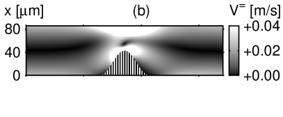
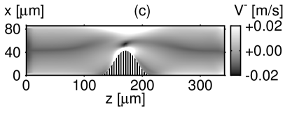
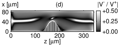
Figure 6: Comparison of (a) $V$ as obtained from a particulate simulation at $\Phi=0.4$ and (b) the reconstruction $V^{=}$ defined in Eq. (3) based on the isotropic shear rate obtained from a non-particulate simulation ($\Phi=0$) with matched viscosity. (c) and (d) show the absolute and relative differences $V^{-}=V^{=}-V$ and $|V^{-}/V^{+}|$ with $V^{+}=V^{=}+V$.

V Conclusions

Boundary conditions suitable for efficient modeling of equilibrated suspension flow through an infinite channel followed by a single stenosis were implemented in a parallel LB code. The time-averaged flow field produced by a coarse-grained particulate blood model was reproduced by a non-particulate model with a matched viscosity. Moreover, the cell-induced plasma velocity fluctuations in the bulk of the suspension can be well understood from a simple dimensional argument and therefore may be reproduced qualitatively from the non-particulate simulation.

A continuous model for blood can be run at reduced resolution and therefore allows to simulate flows in larger geometries more efficiently, stretching to arteries or veins boyd05 ; mikhal12 . The estimate Eq. (3) would allow to equip such models with a qualitative prediction of the RBC-induced plasma velocity fluctuations. The combined model might be useful for studying transport phenomena in geometries inaccessible to the more expensive particulate blood models. In view of these applications the deviations of the continuous model at cell-depleted boundary layers are no serious limitation since these scales would not be resolved in a continuous simulation at a practical spatial resolution. A next important step would be to connect the velocity fluctuations to an effective diffusivity for scalar transport in the medium.

References

- (1) A. L. Zydney and C. K. Colton, PhysicoChem. Hydrodyn. 10, 77 (1988).
- (2) T. Ishikawa and T. Yamaguchi, Phys. Rev. E 77, 041402 (2008).
- (3) F. Janoschek, F. Toschi, and J. Harting, Phys. Rev. E 82, 056710 (2010).
- (4) S. Melchionna, Macromolecular Theory and Simulations 20, 548 (2011).
- (5) J. Boyd, J. Buick, J. A. Cosgrove, and P. Stansell, Phys. Med. Biol. 50, 4783 (2005).
- (6) J. Mikhal and B. J. Geurts, J. Math. Biol., doi:10.1007/s00285-012-0627-5 (2012).
- (7) E. N. Sorensen, G. W. Burgreen, W. R. Wagner, and J. F. Antaki, Annals of Biomedical Engineering 27, 436 (1999).
- (8) T. Ishikawa, N. Kawabata, Y. Imai, K. Tsubota, and T. Yamaguchi, Journal of Biomechanical Science and Engineering 2, 12 (2007).
- (9) S. Succi, The Lattice Boltzmann Equation for Fluid Dynamics and Beyond (Oxford University Press, 2001).
- (10) F. Janoschek, J. Harting, and F. Toschi, Accurate lubrication corrections for spherical and non-spherical particles in discretized fluid simulations. Submitted for publication—preprint at arXiv:1308.6482 (2013).
- (11) P. R. Nott and J. F. Brady, J. Fluid Mech. 275, 157 (1994).
- (12) M. Hecht and J. Harting, J. Stat. Mech. Theor. Exp. 2010, P01018 (2010).
- (13) A. M. Robertson, A. Sequeira, and M. V. Kameneva, Hemodynamical flows (Springer, 2008), p. 63.
- (14) J. Boyd, J. M. Buick, and S. Green, Phys. Fluids 19, 093103 (2007).