Inverse counting statistics for stochastic and open quantum systems: the characteristic polynomial approach

Abstract

We consider stochastic and open quantum systems with a finite number of states, where a stochastic transition between two specific states is monitored by a detector. The long-time counting statistics of the observed realizations of the transition, parametrized by cumulants, is the only available information about the system. We present an analytical method for reconstructing generators of the time evolution of the system compatible with the observations. The practicality of the reconstruction method is demonstrated by the examples of a laser-driven atom and the kinetics of enzyme-catalyzed reactions. Moreover, we propose cumulant-based criteria for testing the non-classicality and non-Markovianity of the time evolution, and lower bounds for the system dimension. Our analytical results rely on the close connection between the cumulants of the counting statistics and the characteristic polynomial of the generator, which takes the role of the cumulant generating function.

1 Introduction

When probing a physical system we often face the problem that only a small part of its evolution is accessible to direct observation. Notably, in some cases, the entire available information consists of observable time-discrete events, indicating that a stochastic transition between two states of the system has been realized. Examples of such events are photons emitted by fluorescent ions [1] or nitrogen-vacancy centers [2], single electrons passing through quantum dots [3, 4, 5], individual steps of processive motor proteins [6] or product molecules generated in enzyme-catalyzed reactions [7, 8, 9]. Common to all is that the observation of the system is restricted to a simple counting process of certain discrete events by a detector.

In this paper we ask the question: What can be learned about the physical system if the counting statistics of these events is the only available information? To be specific, the long-time counting statistics is the discrete probability distribution $p(n)$, expressing the probability that exactly $n$ events occur within a sufficiently long time interval $[0,t]$. The distribution $p(n)$ is conveniently parametrized in terms of its cumulants, where non-zero higher order cumulants indicate deviations from Gaussian behaviour. Our goal is to exploit these deviations in order to recover the hidden structure and evolution of the system from the observational data.

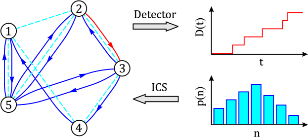
Figure 1: A detector monitors a stochastic transition between two specific states (red arrow) of a system with $N$ states connected by stochastic and quantum transitions (arrows and dashed lines). The long-time counting statistics of the events $p(n)$ obtained from the detector signal $D(t)$ contains sufficient information to reconstruct the generators governing the time evolution of the system.

In answering the above question, we present several results that elucidate the relation between the evolution of the system and the observed counting statistics. Most importantly, we identify the characteristic polynomial of the time-independent generator, governing the time evolution, as the central object of our study. The characteristic polynomial is shown to have two essential properties: First, it can be reconstructed from a finite number of cumulants, and second, it takes the role of the cumulant generating function. As an immediate consequence, we find that for an open quantum system with dimension $N$ at most $2(N^{2}-1)$ cumulants of the observed counting statistics are independent. Building on these results, we further design cumulant-based tests to identify non-classical and non-Markovian time evolutions, and to estimate the system dimension $N$. Moreover, we suggest an analytical method for reconstructing generators compatible with the observations. We find that the result of the reconstruction process is not necessarily unique, i.e., different generators may lead to identical observed counting statistics. By analogy to problems such as inverse scattering theory [10] we refer to our methods collectively as inverse counting statistics (ICS).

The theory of ICS is a new member of a family of methods to discern the properties of a system from observational data. Part of these methods have the objective of reconstructing specific system properties, such as quantum state tomography [11, 12, 13, 14], which addresses the problem of efficiently determining the state of a physical system by measuring a complete set of observables. Various methods, on the other hand, are based on inequalities for selected system properties; these inequalities are tested against experimental observations. The most established test for the non-classicality of the evolution of a system is the Leggett-Garg inequality [15, 16], whose experimental violation was demonstrated with nitrogen-vacancy defects [17] and which may be used to evidence non-classical electron transport in nano-structures [18]. The advantages of cumulant-based inequalities for probing non-classicality of current correlations in mesoscopic junctions and a related cumulant-based Bell test have been recently discussed in Refs. [19, 20]. Furthermore, identifying non-Markovian evolutions has become a subject of increasing interest and several measures of non-Markovianity in quantum systems have been proposed [21, 22, 23]. For determining the dimension of quantum systems, the concept of dimension witness has been introduced [24] and experimentally applied [25]. The dimensionality of stochastic systems in the context of enzyme dynamics was shown to be directly related to the so-called randomness parameter [6, 8, 9].

The theory of ICS is of course related to the methods of full counting statistics (FCS) [26, 27, 28, 29, 30, 31, 32] and large deviation theory [33, 34, 35, 36]. These methods have been successfully applied to a wide range of stochastic and quantum systems, notably in mesoscopic physics [32]. In fact, measurements of higher order cumulants of electronic current fluctuations have been achieved in tunnel junctions [37, 38] and in Coulomb blockaded quantum dots [3, 4, 5]. In general, FCS and large deviation theory are aimed at determining the counting statistics of observable events if the generator of the time evolution and all system parameters are known a priori. Therefore these methods are not directly applicable to the inverse problem considered here.

The structure of this paper is as follows: In section 2 we introduce the underlying model and recall the basics of the theory of FCS. In section 3 we give the details of the methods of ICS by establishing the connection between the characteristic polynomial and the cumulants of the counting statistics. Furthermore, we describe the cumulant-based tests and the analytical method for reconstructing the generator of the time evolution. To illustrate the capacities of ICS we present specific reconstruction examples in section 4. We end with the conclusions in section 5.

2 Model and prerequisites

While keeping the discussion broad we consider a specific system for clarity. This system consists of $N$ orthogonal states, connected by stochastic and quantum transitions (cf. Fig 1). The state of the system is described by the density operator $\rho(t)$ whose time evolution is governed by the master equation

$$\frac{\mathrm{d}}{\mathrm{d}t}\rho(t)=\mathcal{L}\rho(t)\,,$$ (1)

with $\mathcal{L}$ the time-independent Markovian generator. The formal solution of Eq. (1) is given by $\rho(t)=\mathrm{e}^{\mathcal{L}t}\rho(0)$. We focus specifically on the long-time limit of the evolution of the system and presume that Eq. (1) has a unique steady state $\rho_{s}$ defined by $\mathcal{L}\rho_{s}=0$, i.e., the generator $\mathcal{L}$ has a unique zero eigenvalue.

We want our model to cover two scenarios: In the classical limit, the system evolves according to a time-continuous Markov process [39] with only stochastic transitions, whereas in the general case we deal with an open quantum system [40, 41]. The model can also be seen as a continuous-time extension of hidden quantum Markov models studied in Ref. [42]. The generator $\mathcal{L}$ in Lindblad form acts on $\rho$ as

$$\mathcal{L}\rho=-\mathrm{i}[H,\rho]+\sum_{i\neq j}\Big{(}{L}^{\phantom{{\dagger}}}_{ij}\rho{L}^{\dagger}_{ij}-\frac{1}{2}\{{L}^{\dagger}_{ij}{L}^{\phantom{{\dagger}}}_{ij},\rho\}\Big{)}\,,$$ (2)

where ${L}^{\phantom{{\dagger}}}_{ij}$ and ${L}^{\dagger}_{ij}$ are Lindblad operators and $\{\>\,,\>\}$ stands here for the anticommutator. The Lindblad operators are of the form $L_{ij}=\sqrt{\kappa_{ij}}|{i}\rangle\langle{j}|$ and describe stochastic transitions from state $|{j}\rangle$ to state $|{i}\rangle$ with time-independent rates $\kappa_{ij}\geq 0$. The time-independent Hamiltonian operator $H$ is expressed as a Hermitian matrix in the basis $\{|{i}\rangle\}$, fixed by the stochastic transitions. A priori, this model has $2N^{2}-N$ real-valued parameters: $N^{2}-N$ transition rates $\kappa_{ij}$, $(N^{2}-N)/2$ complex-valued off-diagonal elements of $H$, and $N$ real-valued diagonal elements of $H$. For many systems of interest, part of the stochastic or quantum transitions between states are identically zero; the non-zero transitions are conveniently depicted as a graph (cf. Fig 1).

We assume that the detector monitors a single stochastic transition $|{j_{*}}\rangle\rightarrow|{i_{*}}\rangle$ between two selected states $|{j_{*}}\rangle$ and $|{i_{*}}\rangle$ with perfect efficiency. The detector produces a time-continuous signal $D(t)$, containing the number $n\geq 0$ of events observed up to the time $t$ (cf. Fig. 1). The combined state of the system and detector after the $n$-th incoherent event is given by the $n$-resolved density operator $\rho_{n}(t)$, where the additional index specifies the state of the detector [43].

The presented model is applicable to many interesting settings, in particular to stochastic and quantum mechanical transport problems [32, 39]. In this case, $N-1$ states describe different particle configurations and the remaining state is identified with the empty state of the system. Transitions that involve a change in the number of particles are interpreted as particle transfers between the system and external reservoirs, and the detector measures particle currents and fluctuations.

2.1 Established results from FCS

Let us briefly recall useful results from the theory of FCS (see Ref. [31] for details) and define quantities of interest for the rest of the paper. The density operator of the system and detector $\rho_{n}(t)$ satisfies the $n$-resolved master equation $\partial_{t}\rho_{n}(t)=\mathcal{L}^{(0)}\rho_{n}(t)+\mathcal{L}^{(1)}\rho_{n-1}(t)$, where the generator has been separated into two parts as $\mathcal{L}=\mathcal{L}^{(0)}+\mathcal{L}^{(1)}$. In terms of matrix elements, $\mathcal{L}^{(1)}={L}^{\phantom{{\dagger}}}_{i_{*}j_{*}}\rho{L}^{\dagger}_{i_{*}j_{*}}$ contains the only off-diagonal element corresponding to the transition $|{j_{*}}\rangle\rightarrow|{i_{*}}\rangle$ and $\mathcal{L}^{(0)}$ the remaining elements. The finite-difference equation for $\rho_{n}(t)$ is solved by using the discrete Laplace transform $\rho_{\xi}(t)=\sum_{n}\rho_{n}(t)\mathrm{e}^{\xi n}$ which obeys the equation

$$\frac{\mathrm{d}}{\mathrm{d}t}\rho_{\xi}(t)=\mathcal{L}_{\xi}\rho_{\xi}(t)\,,$$ (3)

where the deformed generator $\mathcal{L}_{\xi}=\mathcal{L}^{(0)}+\mathrm{e}^{\xi}\mathcal{L}^{(1)}$ has been introduced. The Fourier transform is often used instead of the Laplace transform, which corresponds to the replacement $\xi\rightarrow\mathrm{i}\xi$ throughout the paper.

A crucial observation of FCS and large deviation theory is that the cumulant generating function $G(\xi)=\log\mathbb{E}\big{[}\mathrm{e}^{\xi D}\big{]}$, where $\mathbb{E}\big{[}\!\cdot\!\big{]}$ stands for the expectation, is connected to the eigenvalue of smallest magnitude $\lambda(\xi)$ of the deformed generator $\mathcal{L}_{\xi}$ through the relation $\lim_{t\rightarrow\infty}G(\xi)/t=\lambda(\xi)$ [33, 36]. In other words, $\lambda(\xi)$ corresponds to the unique zero eigenvalue of $\mathcal{L}$ in the limit $\xi\rightarrow 0$. In the long-time limit, the cumulants $C_{\nu}$ of the probability distribution $p(n)$ of the detector variable $D(t)$ are then given by

$$C_{\nu}=\frac{\partial^{\nu}G(\xi)}{\partial\xi^{\nu}}\bigg{|}_{\xi=0}=t\,\frac{\partial^{\nu}\lambda(\xi)}{\partial\xi^{\nu}}\bigg{|}_{\xi=0}\qquad\nu\geq 1\,.$$ (4)

Using Eq. (4) therefore allows us to determine the counting statistics of the detector variable $D(t)$, in particular its average $\mathbb{E}\big{[}D\big{]}=C_{1}$ and variance ${\rm Var}(D)=C_{2}$, provided that the deformed generator $\mathcal{L}_{\xi}$ is known. Since all cumulants $C_{\nu}$ increase linearly with time $t$, we introduce the scaled cumulants $c_{\nu}=C_{\nu}/t$.

Corresponding results for the purely classical Markov process are obtained by restricting the previous derivations to the occupation probabilities $\rho_{ii}$. It is then convenient to introduce the probability vector $p=\{\rho_{ii},i=1,\ldots,N\}$ and the stochastic generator $\mathcal{L}^{\rm cl}$ acting on $p$. In practice, $\mathcal{L}^{\rm cl}$ and the quantum generator $\mathcal{L}^{\rm qm}$ are represented by $N\times N$ and $N^{2}\times N^{2}$ matrices, respectively, and $\rho=\{\rho_{ij},\,i,j=1,\ldots,N\}$ is a vector in Liouville space with $N^{2}$ components. Unless necessary, we will not explicitly distinguish between stochastic and open quantum systems and consider a generic generator of dimension $M\times M$.

3 Inverse counting statistics

We now present the general theory of ICS, which enables us to analyze the system by using the information provided by measured cumulants. The main results of ICS are of two kinds: The first (§3.3) is formulated as a cumulant-based test for non-classicality, non-Markovianity and system dimension $N$; the second (§3.4) aims at the reconstruction of generator of the time evolution. Both are based on the close relation between the characteristic polynomial of the generator and the cumulants, which will be established first.

3.1 Characteristic polynomial of the generator

Most studies of stochastic or quantum systems focus on the spectrum of the generator, e.g., the Hamiltonian of the system. The characteristic polynomial is rarely used even though it contains the same information as the spectrum provided that the system is finite-dimensional. A notable exception is the polynomial-based approach to quantum mechanical perturbation theory by Raghunathan [44]. The significant advantage of the characteristic polynomial over the spectrum is that it is always possible to obtain analytical expressions for the former. This particular feature will be fully exploited in the following. In contrast, analytical expressions for the spectrum, i.e., the roots of the characteristic polynomial, cannot be found in general.

We here consider the characteristic polynomial $P_{\xi}(x)=\det[x\mathcal{I}-\mathcal{L}_{\xi}]$ of the deformed generator $\mathcal{L}_{\xi}$, with $\mathcal{I}$ the identity matrix. Generally, $P_{\xi}(x)$ of degree $M$ can be written as

$$P_{\xi}(x)=x^{M}+a_{M-1}x^{M-1}+\sum_{\mu=0}^{M-2}a_{\mu}(\xi)x^{\mu}\,.$$ (5)

The coefficients $a_{\mu}(\xi)$ are given by the sum over the principal minors of order $(M-\mu)$ of the deformed generator $\mathcal{L}_{\xi}$ [45, 46] and depend on the variable $\xi$, except for the coefficient $a_{M-1}$. The general expressions for the coefficients $a_{\mu}(\xi)$ are unwieldy, but can be readily calculated for system dimensions of interest. Particularly simple exceptions are $a_{M-1}=-\tr[\mathcal{L}_{\xi}]$ and $a_{0}(\xi)=(-1)^{M}\det[\mathcal{L}_{\xi}]$. Note that each generator $\mathcal{L}_{\xi}$ has a unique characteristic polynomial $P_{\xi}(x)$, whereas to a given generic polynomial there may correspond none, one or several generators $\mathcal{L}_{\xi}$.

In its factored form, $P_{\xi}(x)$ yields the entire spectrum $\sigma_{\xi}$ of the generator, including $\lambda(\xi)$, and it thus contains more information than the cumulant generating function $G(\xi)$. Consequently, generators $\mathcal{L}_{\xi}$ with identical characteristic polynomials $P_{\xi}(x)$ produce the same counting statistics and will be referred to as being equivalent. The characteristic polynomial is therefore perfectly suited for studying symmetries with respect to transformations of $\mathcal{L}_{\xi}$ that leave the counting statistics unchanged. Specifically, $P_{\xi}(x)$ is invariant under arbitrary similarity transformations of the generator $\mathcal{L}_{\xi}\rightarrow T^{-1}\mathcal{L}_{\xi}T$. However, the structure of $\mathcal{L}_{\xi}$ imposed by Eq. (2) is not preserved under similarity transformations, i.e., the transformed matrix is generally not a valid generator. Structure-preserving transformations are, for instance, permutations applied to the matrix elements of $\mathcal{L}_{\xi}$. These transformations preserve the characteristic polynomial $P_{\xi}(x)$ and the structure of $\mathcal{L}_{\xi}$.

It is instructive to consider the example of a stochastic system with unidirectional transitions between nearest-neighbours, i.e., $\kappa_{i+1,i}>0$ for $i=1,\ldots,N$ with periodic boundary conditions and all other rates zero. In this case, the generator $\mathcal{L}_{\xi}^{\rm cl}$ is a triangular matrix, except for a single element, and has the characteristic polynomial

$$P^{\rm cl}_{\xi}(x)=(-1)^{N}\left[\,\prod_{i=1}^{N}(x+\kappa_{i+1,i})-\mathrm{e}^{\xi}\prod_{i=1}^{N}\kappa_{i+1,i}\right].$$ (6)

Clearly, $P^{\rm cl}_{\xi}(x)$ is invariant under any permutation of the rates $\kappa_{i+1,i}$ and hence there are $N!$ equivalent generators related by permutations which yield identical counting statistics. In addition, the statistics of the observations is independent of the position of the detector.

3.2 Reconstruction of characteristic polynomials from cumulants

The characteristic polynomial $P_{\xi}(x)$ plays an important role in ICS since it can be reconstructed from a finite number of cumulants. Reconstructing the full generating function $G(\xi)$ from cumulants, for example, by exploiting Eq. (4), may be possible for a few special cases. To our knowledge there is however no general method available.

To start with, we parametrize $P_{\xi}(x)$ in a more convenient way. In view of the local dependence of the cumulants $c_{\nu}$ on the eigenvalue $\lambda(\xi)$ according to Eq. (4) we constrain our analysis to the properties of $P_{\xi}(x)$ in the vicinity of $\xi=0$. We consider the Taylor expansion of the coefficients $a_{\mu}(\xi)$ around $\xi=0$, which yields

$$P_{\xi}(x)=x^{M}+a_{M-1}x^{M-1}+\sum_{\mu=0}^{M-2}\sum_{k=0}^{\infty}\frac{a_{\mu}^{(k)}\xi^{k}}{k!}\,x^{\mu}\,,$$ (7)

with the shorthand notation $a_{\mu}^{(k)}\equiv\partial_{\xi}^{k}a_{\mu}(\xi)|_{\xi=0}$ and in particular $a_{\mu}\equiv a_{\mu}(\xi)|_{\xi=0}$. Since $a_{\mu}(\xi)$ depends on $\xi$ only through the factor $\mathrm{e}^{\xi}$ in the generator $\mathcal{L}_{\xi}$ we find that $a_{\mu}^{(k)}=a_{\mu}^{(1)}\equiv a_{\mu}^{\prime}$ for all $k\geq 2$. After simplifying Eq. (7) we can rewrite $P_{\xi}(x)$ in the compact form

$$P_{\xi}(x)=P_{\xi}(x)\big{|}_{\xi=0}+\partial_{\xi}P_{\xi}(x)\big{|}_{\xi=0}\,(\mathrm{e}^{\xi}-1)\,.$$ (8)

The characteristic polynomial $P_{\xi}(x)$ in the vicinity of $\xi=0$ is thus fully determined by the pair of polynomials $P_{\xi}(x)|_{\xi=0}$ and $\partial_{\xi}P_{\xi}(x)|_{\xi=0}$, or equivalently parametrized by $2(M-1)$ of the coefficients $a_{\mu}$ and $a_{\mu}^{\prime}$, with $\mu=0,\ldots,M$. Explicitly, the polynomials $P_{\xi}(x)\big{|}_{\xi=0}$ and $\partial_{\xi}P_{\xi}(x)\big{|}_{\xi=0}$ are specified by the two sets of $M-1$ coefficients $\{a_{1},\ldots,a_{M-1}\}$ and $\{a_{0}^{\prime},\ldots,a_{M-2}^{\prime}\}$, respectively, where we have taken into account that $a_{0}=a_{M-1}^{\prime}=a_{M}^{\prime}=0$ and $a_{M}=1$ are fixed.

Next, the direct relation between the cumulants $c_{\nu}$ and the characteristic polynomial $P_{\xi}(x)$ is established. We note that the equality $P_{\xi}[\lambda(\xi)]=0$ holds by definition of the characteristic polynomial. By repeatedly taking the total derivative of this equality with respect to $\xi$ and evaluating it at $\xi=0$, we can generate the (infinite) set of equations

$$h_{\ell}(a_{\mu},a_{\mu}^{\prime},c_{\nu})\equiv\frac{\mathrm{d}^{\ell}P_{\xi}[\lambda(\xi)]}{\mathrm{d}\xi^{\ell}}\bigg{|}_{\xi=0}=0\qquad\ell\geq 1\,.$$ (9)

We observe that Eqs. (9) relate the quantities $a_{\mu}$, $a^{\prime}_{\mu}$ and $c_{\nu}$, taking account of the relations $c_{\nu}=\partial^{\nu}_{\xi}\lambda(\xi)|_{\xi=0}$ for $\nu\geq 1$ and $\lambda(\xi)|_{\xi=0}=0$. For instance, the first three functions $h_{\ell}(a_{\mu},a_{\mu}^{\prime},c_{\nu})$ are given by

$$\eqalign{h_{1}&=a_{0}^{\prime}+a_{1}c_{1}\,,\\ h_{2}&=a_{0}^{\prime}+a_{1}c_{2}+2a_{1}^{\prime}c_{1}+2a_{2}c_{1}^{2}\,,\\ h_{3}&=a_{0}^{\prime}+a_{1}c_{3}+3a_{1}^{\prime}(c_{1}+c_{2})+6a_{2}c_{1}c_{2}+6a_{2}^{\prime}c_{1}^{2}+6a_{3}c_{1}^{3}\,.}$$ (10)

As can be seen from Eq. (8) each function $h_{\ell}$ is linear in the coefficients $a_{\mu}$, $a_{\mu}^{\prime}$. Moreover, considering $h_{\ell}$ as a function of $a_{\mu}$ and $a_{\mu}^{\prime}$, we observe that only $h_{\ell}$ with $\ell\geq\mu$ depend on the coefficient $a_{\mu}$, and consequently all $h_{\ell}$ with $\ell=1,\ldots,M$ are linearly independent, regardless of the values of the $c_{\nu}$. Lastly, Eqs. (9) are inhomogeneous for $\ell\geq M$ because constant terms are generated by the term $\lambda^{M}(\xi)$.

Using Eqs. (9) we can reconstruct the characteristic polynomial $P_{\xi}(x)$ from the first $2(M-1)$ cumulants $c_{\nu}$. To this end, we choose the first $2(M-1)$ equations $h_{\ell}(a_{\mu},a_{\mu}^{\prime},c_{\nu})=0$ with the cumulants $c_{\nu}$ as fixed arguments and solve the resulting linear system for the coefficients $a_{\mu}$, $a_{\mu}^{\prime}$. Aside from exceptional cases, the linear system has a unique solution for the $2(M-1)$ coefficients $a_{\mu}$ and $a_{\mu}^{\prime}$, thereby yielding a unique $P_{\xi}(x)$. We stress that the reconstruction of the characteristic polynomial $P_{\xi}(x)$ does not guarantee the existence of a generator $\mathcal{L}_{\xi}$ compatible with the first $2(M-1)$ cumulants $c_{\nu}$. However, if the cumulants $c_{\nu}$ indeed result from an evolution governed by a generator $\mathcal{L}_{\xi}$ then the reconstructed $P_{\xi}(x)$ is the unique characteristic polynomial of $\mathcal{L}_{\xi}$.

From the reconstructed charateristic polynomial $P_{\xi}(x)$ all cumulants of higher order $c_{\nu}$, with $\nu>2(M-1)$, can be found. One way of doing so is to evaluate $\lambda(\xi)$, equivalent to the generating function $G(\xi)$, and subsequently use Eq. (4). We now introduce a direct analytical method, which again is based solely on $P_{\xi}(x)$ and thus avoids the evaluation of $G(\xi)$. Instead of solving Eqs. (9) for the coefficients $a_{\mu}$, $a_{\mu}^{\prime}$ with fixed cumulants $c_{\nu}$, we assume that the coefficients are known and solve Eqs. (9) recursively for the cumulants $c_{\nu}$. We illustrate the procedure by evaluating the first three (scaled) cumulants, the average, variance and skewness:

$$\eqalign{c_{1}&=-\frac{a_{0}^{\prime}}{a_{1}}\,,\\ c_{2}&=-\frac{a_{0}^{\prime}+2a_{1}^{\prime}c_{1}+2a_{2}c_{1}^{2}}{a_{1}}\,,\\ c_{3}&=-\frac{a_{0}^{\prime}+3a_{1}^{\prime}c_{1}+6a_{2}^{\prime}c_{1}^{2}+6a_{3}c_{1}^{3}+3a_{1}^{\prime}c_{2}+6a_{2}c_{1}c_{2}}{a_{1}}\,,\\ }$$ (11)

where cumulants $c_{\nu}$ are expressed in terms of $a_{\mu}$, $a_{\mu}^{\prime}$ and cumulants $c_{\eta}$ with $\eta<\nu$.

In summary, we have two complementary methods at our disposal, which enable us (i) to reconstruct $P_{\xi}(x)$ from a finite number of cumulants and (ii) to find all cumulants from a given $P_{\xi}(x)$. The characteristic polynomial $P_{\xi}(x)$ thus completely replaces the cumulant generating function $G(\xi)$. This remarkable property also suggests an alternative to the standard methods of FCS: Evaluating (zero-frequency) cumulants within FCS usually requires the calculation of the eigenvalue $\lambda(\xi)$ or the regular part of the resolvant of $\mathcal{L}_{\xi}$ [31]. In this traditional way, analytical results can only be obtained for small system dimensions. In contrast, our polynomial-based procedure is efficient and direct: It suffices to calculate $P_{\xi}(x)$ for a given $\mathcal{L}_{\xi}$, which yields the coefficients $a_{\mu}\equiv a_{\mu}(\xi)|_{\xi=0}$ and $a_{\mu}^{\prime}\equiv\partial_{\xi}a_{\mu}(\xi)|_{\xi=0}$, and then to use Eqs. (11). Analytical results for all cumulants $c_{\nu}$ can be obtained for any generator $\mathcal{L}_{\xi}$ regardless of the system dimension, including $\mathcal{L}_{\xi}$ with more general Lindblad operators than in Eq. (2). In particular, the Fano factor

$$F\equiv\frac{c_{2}}{c_{1}}=1+\frac{2a_{0}^{\prime}a_{2}}{a_{1}^{2}}-\frac{2a_{1}^{\prime}}{a_{1}}$$ (12)

is readily found in this way. In general, calculating cumulants recursively seems to be more efficient than finding the full cumulant generating function $G(\xi)$. Recursive schemes for calculating cumulants of high orders have also been exploited in traditional FCS [29, 30, 31].

3.3 Tests for non-classicality, non-Markovianity and system dimension

Table 1: We design several tests based on the fact that the number of independent cumulants is at most $N_{p}$. If more than $N_{p}$ independent cumulants are observed in an experiment we can discard the hypothesis under given prior assumptions.

Prior Assumptions	Hypothesis
Markovian, Dimension $N$	Classicality
Classical, Dimension $N$	Markovianity
Quantum, Dimension $N$	Markovianity
Classical, Markovian	Dimension $N$
Quantum, Markovian	Dimension $N$

The reconstruction of the characteristic polynomial makes it possible to design tests for distinguishing between different types of evolutions and system dimensions. The tests are based on the observation that for a finite-dimensional Markovian system, with the Lindblad evolution according to Eq. (2), the number of independent cumulants is finite. Indeed, as shown previously, $P_{\xi}(x)$ can be reconstructed from the first $N_{p}=2(M-1)$ cumulants and serves as a cumulant generating function. Thus, the number of independent cumulants is at most $N_{p}$. The specific value of $N_{p}$ depends on the assumptions about the underlying model as regarding classicality, Markovianity and system dimension. If now one of the assumptions is considered on the level of a hypothesis and the number of independent cumulants exceeds the upper limit $N_{p}$, we can reject this initial hypothesis.

As a concrete example, consider a system with two dimensions and Markovian dynamics (‘assumptions’). We want to test whether the dynamics is classical (‘hypothesis’) or not. The system may describe a resonance fluorescence experiment with trapped ions [1] or nitrogen-vacancy centers [2], in which the counting statistics of emitted photons is analyzed. Suppose the available cumulants are $\tilde{c}_{1}$, $\tilde{c}_{2}$ and $\tilde{c}_{3}$, where the tilde marks quantities obtained from measurements. Given $\tilde{c}_{1}$ and $\tilde{c}_{2}$, and under the hypothesis that the dynamics is classical we find from Eqs. (10) for the classical case with $M=N$

$$\tilde{P}^{\rm cl}_{\xi}(x)=x^{2}+\frac{2\tilde{c}_{1}^{2}}{\tilde{c}_{1}-\tilde{c}_{2}}x-\frac{2\tilde{c}_{1}^{3}}{\tilde{c}_{1}-\tilde{c}_{2}}(\mathrm{e}^{\xi}-1)\,.$$ (13)

The predicted classical value of the third cumulant $c^{\rm cl}_{3}=\tilde{c}_{1}+3\tilde{c}_{2}(\tilde{c}_{2}/\tilde{c}_{1}-1)$ then follows from Eq. (11). If the predicted and measured value differ, i.e., $c^{\rm cl}_{3}\neq\tilde{c}_{3}$, then the dynamics of the system is necessarily non-classical. This conclusion relies on the prior assumption that the system is two-dimensional and Markovian, but the argument can be immediately adapted to different combinations of assumptions and hypotheses, as summarized in Table 1. The generic structure of the test is as follows:

1. The first $N_{p}+1$ cumulants of the counting statistics are measured.

2. From the first $N_{p}$ cumulants the characteristic polynomial $P_{\xi}(x)$ is reconstructed in accord with the prior assumptions (classicality, Markovianity or system dimension).

3. The cumulant $c_{N_{p}+1}$ is predicted from $P_{\xi}(x)$ and compared to the measured value of $c_{N_{p}+1}$.

4. If the predicted and measured value of $c_{N_{p}+1}$ differ then the measured cumulant is independent from the lower-order cumulants. Therefore the dynamics of the system cannot be generated by $\mathcal{L}_{\xi}$ and the hypothesis is discarded.

Inevitable experimental uncertainties lead of course to probabilistic rather than sharp test results; however, the result can always be corroborated by measuring and comparing more high-order cumulants and/or using a longer time base for the measurement.

Note that the test does not verify the existence of a generator $\mathcal{L}_{\xi}$ compatible with the first $N_{p}$ cumulants; this problem is addressed in the next section. As a consequence, the predicted and measured values of $c_{N_{p}+1}$ can differ for two reasons: Either the generator $\mathcal{L}_{\xi}$ compatible with the first $N_{p}$ cumulants makes a false prediction about the measurement result, or the generator does not exist, also leading to a false prediction. In fact, the existence of a characteristic polynomial compatible with measurements already imposes restrictions on the cumulants. We see from Eq. (13), for instance, that for the classical two-state system it is required that $\tilde{c}_{1}\neq\tilde{c}_{2}$. Moreover, as pointed out in Ref. [24], one can only provide a lower bound on the unknown dimension of the system. In our case, the test reveals that the system dimension must be at least $N_{p}+1$ and consequently we cannot test for arbitrary dimensions $N$.

3.4 Reconstruction of generators from characteristic polynomials

Even though $P_{\xi}(x)$ contains essential information about the system, it is still desirable to reconstruct the generator $\mathcal{L}_{\xi}$ from cumulants. By using the generator together with Eq. (1) we can determine the full time evolution of the system and the steady state $\rho_{s}$. The reconstruction furthermore allows us to find restrictions imposed on the cumulants that warrant the existence of a generator.

For the reconstruction we have to solve the following inverse problem: Find the values of the parameters entering the structured generator $\mathcal{L}_{\xi}$ such that it reproduces the observed cumulants $\tilde{c}_{\nu}$. The necessary and sufficient condition for $\mathcal{L}_{\xi}$ to generate the cumulants $\tilde{c}_{\nu}$ is

$$P_{\xi}(x)=\tilde{P}_{\xi}(x)\,,$$ (14)

where $\tilde{P}_{\xi}(x)$ is the reconstructed characteristic polynomial and $P_{\xi}(x)$ is the characteristic polynomial of $\mathcal{L}_{\xi}$. We recall that while $P_{\xi}(x)$ is invariant under similarity transformations, the structured generator $\mathcal{L}_{\xi}$ is not, which restricts the number of solutions to the inverse problem considerably.

Let us outline the direct analytical approach to solving the inverse problem. We exploit the fact that analytical expressions are available for $P_{\xi}(x)$ and hence for the coefficients $a_{\mu}$, $a_{\mu}^{\prime}$. The latter are multivariate polynomials of degree $M-\mu$ in the parameters of the model; the parameters are collected into the set $S$ for convenience. Equation (14) is thus equivalent to the system of $2(M-1)$ polynomial equations

$$\eqalign{a_{\mu}(S)&=\tilde{a}_{\mu}\,,\\ a_{\mu}^{\prime}(S)&=\tilde{a}_{\mu}^{\prime}\,.}$$ (15)

From a geometrical point of view, each equation defines an algebraic variety in the parameter space corresponding to $S$, and the solution of Eqs. (15) is given by the intersection of these varieties [47, 48].

It is not necessarily the case that all polynomial equations (15) are algebraically independent, which can be checked, in principle, by using the standard methods of algebraic geometry [47, 48]. To take this into account we introduce $N_{i}\leq 2(M-1)$, the number of algebraically independent equations. If the number of parameters $|S|$ is larger than $N_{i}$, the generator $\mathcal{L}_{\xi}$ cannot be determined by our approach. Otherwise, if $|S|\leq N_{i}$, we can determine all structured $\mathcal{L}_{\xi}$ compatible with Eq. (14) in two steps: First, we select $|S|$ independent equations from Eqs. (15) and solve the resulting polynomial system, which reduces the original solution space to a finite discrete set, denoted $B$. Subsequently, we discard all solutions in $B$ that do not satisfy the full set of Eqs. (15), which finally leaves us with the solutions of the inverse problem.

The first step results in the polynomial system

$$\eqalign{a_{\alpha}(S)&=\tilde{a}_{\alpha}\,,\\ a_{\beta}^{\prime}(S)&=\tilde{a}_{\beta}^{\prime}\,,}$$ (16)

where the indices $\alpha,\beta\in\{0,\ldots,M-1\}$ are used to select $|S|$ of the $N_{i}$ independent polynomial equations. In practice, it is advisable to select polynomials with the smallest possible degrees for solving Eqs. (16). At this point, we invoke Bézout’s theorem [47, 48], stating that Eqs. (16) generally have a finite number of solutions, forming the set $B$. More precisely, if we admit complex solutions, the number of distinct solutions is at most $\prod_{k}d_{k}$, where $d_{k}$ is the degree of each polynomial in Eqs. (16). This upper bound scales as $|S|!$ and therefore increases faster than exponentially with the system dimension $N$. The number of solutions can however be significantly reduced by initially restricting the parameter space, most importantly, to real-valued solutions for stochastic systems.

After selecting from $B$ all solutions that solve the full set of Eqs. (15) we are left with zero, one or a finite number of solutions. No valid solution indicates that the underlying model is not compatible with the observed cumulants $\tilde{c}_{\nu}$, e.g., false assumptions are made about the dimension $N$. More than one solution is found if several equivalent generators exist, which by definition cannot be distinguished by the detector. Additional information about the system, such as state occupation probabilities, can be used to single out a unique generator $\mathcal{L}_{\xi}$. Alternatively, several independent detectors can be employed to reduce the number of solutions.

3.5 Embedding of the classical into a quantum model

The dimension of $\mathcal{L}_{\xi}$ is an important factor in the reconstruction because it sets the number of conditions in Eqs. (15) and hence an upper bound for $N_{i}$. The number of conditions scales as $N$ for classical systems and $N^{2}$ for quantum systems, whereas the number of parameters $|S|$ typically scales as $N^{2}$ in both cases. Therefore, ICS applied to classical systems seems to be limited to small dimensions because of the condition $|S|\leq N_{i}$.

We can avoid this problem to some extent by treating the classical system as quantum with a trivial Hamiltonian $H\equiv 0$ in Eq. (2), thereby embedding the classical into a quantum model. The resulting quantum generator $\mathcal{L}^{\rm qm}_{\xi}$, according to Eq. (2), for an actual classical system is sparse and block diagonal, i.e., $\mathcal{L}^{\rm qm}_{\xi}$ separates into the block $\mathcal{L}^{\rm cl}_{\xi}$ and the diagonal block $\mathcal{L}^{\rm coh}_{\xi}$ for the coherences, as exemplified by the generator in Eq. (27). The block $\mathcal{L}^{\rm coh}_{\xi}$ contains elements stemming from the terms $-\frac{1}{2}\{{L}^{\dagger}_{ij}{L}^{\phantom{{\dagger}}}_{ij},\rho\}$ in Eq. (2), which in the long-time limit destroy all coherences $\rho_{i\neq j}$ that may exist initially. As a consequence, the steady-state evolutions resulting from the generators $\mathcal{L}^{\rm qm}_{\xi}$ and $\mathcal{L}^{\rm cl}_{\xi}$ are the same, and the steady-state coherences are identically zero.

The point of interest for the reconstruction is of course the relation between the classical characteristic polynomial $P^{\rm cl}_{\xi}(x)$ and quantum mechanical polynomial $P^{\rm qm}_{\xi}(x)$ obtained from the embedding. The characteristic polynomial of the block-structured generator $\mathcal{L}^{\rm qm}_{\xi}$ factorizes as

$$P^{\rm qm}_{\xi}(x)=P^{\rm cl}_{\xi}(x)P^{\rm coh}_{\xi}(x)\,.$$ (17)

The additional conditions we gain from treating the classical system as quantum mechanical therefore originate from the polynomial $P^{\rm coh}_{\xi}(x)$, which can be made explicit by writing Eq. (14) in two parts as $P^{\rm cl}_{\xi}(x)=\tilde{P}^{\rm cl}_{\xi}(x)$ and $P^{\rm coh}_{\xi}(x)=\tilde{P}^{\rm coh}_{\xi}(x)$.

In practice, starting from $2(N-1)$ measured cumulants of the classical system we reconstruct $\tilde{P}^{\rm cl}_{\xi}(x)$, and in turn generate the first $2(N^{2}-1)$ cumulants. Using these $2(N^{2}-1)$ cumulants we then proceed as for a quantum system to find the rates $\kappa_{ij}$. In this way, the embedding strategy extends the use of ICS to classical systems of larger dimension.

4 Practical reconstruction examples

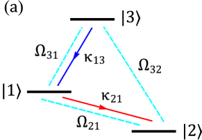
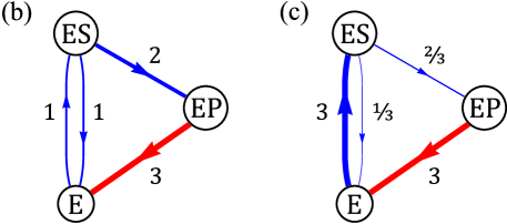
Figure 2: The counting statistics of the monitored stochastic transition (red arrow) is used the reconstruct the generator of the time evolution. (a) Three atomic states in $\Lambda$-type configuration are connected by stochastic and coherent transitions (arrows and dashed lines). The statistics of the spontaneous decay of state $|{1}\rangle$ is used to determine the decay rates $\kappa_{21}$, $\kappa_{13}$ and Rabi frequencies $\Omega_{32}$, $\Omega_{21}$, $\Omega_{31}$. (b) An enzyme-catalyzed reaction is modelled by stochastic transitions (arrows) between three states: empty enzyme $({\rm E})$, enzyme-substrate complex $({\rm ES})$ and enzyme-product complex $({\rm EP})$. The counting statistics of the product molecules is used to determine the transition rates. The observed statistics is identical for the two sets of rates shown in (b) and (c).

We illustrate the reconstruction of generators with concrete examples. For the stochastic two-state system, we present the general solutions of Eqs. (16) in terms of the measured cumulants $\tilde{c}_{\nu}$. As further examples we consider a laser-driven atomic system and the Michaelis-Menten kinetics of enzymatic reactions. In the latter cases, we produce the first $2(N^{2}-1)$ cumulants for a fixed set of parameters and afterwards reconstruct generators $\mathcal{L}_{\xi}$ compatible with these cumulants. Incidentally, this application of ICS constitutes a general method for either verifying the uniqueness of a generator or revealing symmetries of the system that are not immediately apparent from the characteristic polynomial $P_{\xi}(x)$. An example for the characteristic polynomial approach in connection with traditional FCS will be presented elsewhere [49].

4.1 Stochastic two-state system

We first reconsider the classical two-state system with the detector at the transition $|{1}\rangle\rightarrow|{2}\rangle$. The corresponding generator reads

$$\mathcal{L}_{\xi}^{\rm cl}=\bigg{(}\begin{array}[]{cc}-\kappa_{21}&\kappa_{12}\\ \mathrm{e}^{\xi}\kappa_{21}&-\kappa_{12}\end{array}\bigg{)}$$ (18)

and the characteristic polynomial is

$$P_{\xi}^{\rm cl}=x^{2}+(\kappa_{21}+\kappa_{12})x-\kappa_{21}\kappa_{12}(\mathrm{e}^{\xi}-1)\,.$$ (19)

The reconstructed characteristic polynomial $\tilde{P}_{\xi}(x)$ is given by Eq. (13). To find the parameters $S=\{\kappa_{21},\kappa_{12}\}$ of the generator $\mathcal{L}_{\xi}^{\rm cl}$ we have to solve Eq. (16), i.e., the polynomial system

$$\tilde{a}_{1}=\kappa_{21}+\kappa_{12}=\frac{2\tilde{c}_{1}^{2}}{\tilde{c}_{1}-\tilde{c}_{2}}\,,\qquad\tilde{a}_{0}^{\prime}=-\kappa_{21}\kappa_{12}=-\frac{2\tilde{c}_{1}^{3}}{\tilde{c}_{1}-\tilde{c}_{2}}\,,$$ (20)

with the solutions $\{\kappa_{21},\kappa_{12}\}=\{\kappa_{+},\kappa_{-}\}$ and $\{\kappa_{21},\kappa_{12}\}=\{\kappa_{-},\kappa_{+}\}$, where

$$\kappa_{\pm}=\frac{\tilde{c}_{1}^{2}\pm\tilde{c}_{1}^{3/2}\sqrt{2\tilde{c}_{2}-\tilde{c}_{1}}}{\tilde{c}_{1}-\tilde{c}_{2}}\,.$$ (21)

The fact that we obtain two solutions is in agreement with Bézout’s theorem and reflected in the symmetry of the characteristic polynomial $P_{\xi}^{\rm cl}$, which is a special case of Eq. (6). It follows from Eq. (21) that a classical generator $\mathcal{L}_{\xi}^{\rm cl}$ exists for cumulants restricted to the regime $\tilde{c}_{1}>\tilde{c}_{2}\geq\frac{1}{2}\tilde{c}_{1}$. In particular, there is no generator $\mathcal{L}_{\xi}^{\rm cl}$ corresponding to an observed super-Poissonian ($\tilde{c}_{2}>\tilde{c}_{1}$) counting statistics.

4.2 Laser-driven atom with spontaneous decay

We next consider a three atomic states in a $\Lambda$-type configuration [50], where the counting statistics is obtained by observing emitted photons (cf. Fig. 2). The three states $|{1}\rangle$, $|{2}\rangle$ and $|{3}\rangle$ are connected by coherent transitions, parametrized by the Rabi frequencies $\Omega_{ij}$. We assume that the on-site energies of the states are negligible, as is the case for near-resonant laser-driving, so that the Hamiltonian $H$ has the form

$$H=\frac{1}{2}\sum_{i>j}\Omega_{ij}\left(|{i}\rangle\langle{j}|+|{j}\rangle\langle{i}|\right)\,.$$ (22)

Spontaneous decay is modelled by the stochastic transitions $|{3}\rangle\rightarrow|{1}\rangle$ and $|{1}\rangle\rightarrow|{2}\rangle$ with decay rates $\kappa_{13}$ and $\kappa_{21}$, respectively, where the latter is monitored by the detector. The generator of the evolution of the density matrix $\rho=\{\rho_{11},\rho_{12},\ldots,\rho_{33}\}$ reads

$$\mathcal{L}_{\xi}^{\rm qm}=\left(\begin{array}[]{ccccccccc}-\kappa_{21}&\frac{\mathrm{i}}{2}\Omega_{21}&\frac{\mathrm{i}}{2}\Omega_{31}&-\frac{\mathrm{i}}{2}\Omega_{21}&0&0&-\frac{\mathrm{i}}{2}\Omega_{31}&0&\kappa_{13}\\ \frac{\mathrm{i}}{2}\Omega_{21}&-\frac{1}{2}\kappa_{21}&\frac{\mathrm{i}}{2}\Omega_{32}&0&-\frac{\mathrm{i}}{2}\Omega_{21}&0&0&-\frac{\mathrm{i}}{2}\Omega_{31}&0\\ \frac{\mathrm{i}}{2}\Omega_{31}&\frac{\mathrm{i}}{2}\Omega_{32}&-\frac{1}{2}\delta&0&0&-\frac{\mathrm{i}}{2}\Omega_{21}&0&0&-\frac{\mathrm{i}}{2}\Omega_{31}\\ -\frac{\mathrm{i}}{2}\Omega_{21}&0&0&-\frac{1}{2}\kappa_{21}&\frac{\mathrm{i}}{2}\Omega_{21}&\frac{\mathrm{i}}{2}\Omega_{31}&-\frac{\mathrm{i}}{2}\Omega_{32}&0&0\\ \mathrm{e}^{\xi}\kappa_{21}&-\frac{\mathrm{i}}{2}\Omega_{21}&0&\frac{\mathrm{i}}{2}\Omega_{21}&0&\frac{\mathrm{i}}{2}\Omega_{32}&0&-\frac{\mathrm{i}}{2}\Omega_{32}&0\\ 0&0&-\frac{\mathrm{i}}{2}\Omega_{21}&\frac{\mathrm{i}}{2}\Omega_{31}&\frac{\mathrm{i}}{2}\Omega_{32}&-\frac{1}{2}\kappa_{13}&0&0&-\frac{\mathrm{i}}{2}\Omega_{32}\\ -\frac{\mathrm{i}}{2}\Omega_{31}&0&0&-\frac{\mathrm{i}}{2}\Omega_{32}&0&0&-\frac{1}{2}\delta&\frac{\mathrm{i}}{2}\Omega_{21}&\frac{\mathrm{i}}{2}\Omega_{31}\\ 0&-\frac{\mathrm{i}}{2}\Omega_{31}&0&0&-\frac{\mathrm{i}}{2}\Omega_{32}&0&\frac{\mathrm{i}}{2}\Omega_{21}&-\frac{1}{2}\kappa_{13}&\frac{\mathrm{i}}{2}\Omega_{32}\\ 0&0&-\frac{\mathrm{i}}{2}\Omega_{31}&0&0&-\frac{\mathrm{i}}{2}\Omega_{32}&\frac{\mathrm{i}}{2}\Omega_{31}&\frac{\mathrm{i}}{2}\Omega_{32}&-\kappa_{13}\\ \end{array}\right),$$

with $\delta=\kappa_{21}+\kappa_{13}$, from which the (albeit large) analytical expression for the characteristic polynomial $P_{\xi}^{\rm qm}(x)$ is readily found.

For the set of dimensionless decay rates and Rabi frequencies $\{\kappa_{21},\kappa_{13},\Omega_{32},\Omega_{21},\Omega_{31}\}=\{5,4,3,2,1\}$ we produce the first $16$ cumulants $\tilde{c}_{\nu}=\{0.98,0.35,-0.04,\ldots\}$. These are used to reconstruct the characteristic polynomial $\tilde{P}_{\xi}^{\rm qm}(x)$ in terms of the coefficients $\tilde{a}_{\mu}$ and $\tilde{a}_{\mu}^{\prime}$. As a possible choice for the polynomial system in Eq. (16) we select the five polynomial equations

$$\qquad\eqalign{\tilde{a}_{6}^{\prime}=-\frac{1}{2}\kappa_{21}\Omega_{21}^{2}\,,\\ \tilde{a}_{5}^{\prime}=-\frac{3}{2}\kappa_{13}\kappa_{21}\Omega_{21}^{2}-\frac{1}{2}\kappa_{13}\kappa_{21}\Omega_{32}^{2}-\frac{3}{4}\kappa_{21}^{2}\Omega_{21}^{2}\,,\\ \tilde{a}_{8}=3(\kappa_{13}+\kappa_{21})\,,\phantom{\frac{1}{1}}\\ \tilde{a}_{7}=\frac{7}{2}(\kappa_{21}^{2}+\kappa_{13}^{2})+\frac{17}{2}\kappa_{13}\kappa_{21}+\frac{3}{2}(\Omega_{31}^{2}+\Omega_{32}^{2}+\Omega_{21}^{2})\,,\\ \tilde{a}_{6}=4(\kappa_{21}\Omega_{32}^{2}+\kappa_{13}\Omega_{21}^{2})+\frac{37}{4}(\kappa_{21}\kappa_{13}^{2}+\kappa_{13}\kappa_{21}^{2})+\frac{13}{4}(\kappa_{21}\Omega_{31}^{2}+\kappa_{13}\Omega_{32}^{2})\\ \qquad+\>2(\kappa_{13}^{3}+\kappa_{21}^{3})+\frac{11}{4}(\kappa_{21}\Omega_{21}^{2}+\kappa_{13}\Omega_{31}^{2})\,.\\ }$$ (23)

The original parameters of the model are recovered by solving Eqs. (23), however, with all possible sign changes of the Rabi frequencies, i.e., $\{\kappa_{21},\kappa_{13},\Omega_{32},\Omega_{21},\Omega_{31}\}=\{5,4,\pm 3,\pm 2,\pm 1\}$. It can be immediately verified that the characteristic polynomial $P^{\rm qm}_{\xi}(x)$ and Eqs. (23) depend only on the square of the Rabi frequencies, which results in the sign symmetry with eight equivalent generators. The example illustrates that by observing the spontaneous decay of state $|{1}\rangle$ we can determine the magnitude of all Rabi frequencies $\Omega_{ij}$ and spontaneous decay rates $\kappa_{ij}$ of the atomic system.

4.3 Michaelis-Menten kinetics with fluorescent product molecules

Finally, we apply ICS to enzymatic reactions that are described by the Michaelis-Menten kinetics [7, 8, 9]. The kinetics of a single enzyme can be modelled by a stochastic three-state system, where the states correspond to empty enzyme $({\rm E})\equiv|{1}\rangle$, the enzyme-substrate complex $({\rm ES})\equiv|{2}\rangle$ and the enzyme-product complex $({\rm EP})\equiv|{3}\rangle$ [51]. The enzyme-substrate binding is a reversible process while the other transitions are assumed to be unidirectional (cf. Fig. 2). The counting statistics is obtained from monitoring the transition $({\rm EP})\rightarrow({\rm E})$ through the detection of single fluorescent product molecules [7].

For this biological scenario, we produce cumulants for the dimensionless rates $\{\kappa_{21},\kappa_{12},\kappa_{32},\kappa_{13}\}=\{1,1,2,3\}$ with the detector at the transition $|{3}\rangle\rightarrow|{1}\rangle$. Considering the system as being classical we obtain the generator

$$\mathcal{L}_{\xi}^{\rm cl}=\left(\begin{array}[]{ccc}-\kappa_{21}&\kappa_{12}&\mathrm{e}^{\xi}\kappa_{13}\\ \kappa_{21}&-\kappa_{12}-\kappa_{32}&0\\ 0&\kappa_{32}&-\kappa_{13}\\ \end{array}\right)$$ (24)

and the characteristic polynomial

$$\qquad\eqalign{P_{\xi}^{\rm cl}&=x^{3}+(\kappa_{12}+\kappa_{13}+\kappa_{21}+\kappa_{32})x^{2}+(\kappa_{12}\kappa_{13}+\kappa_{13}\kappa_{21}+\kappa_{13}\kappa_{32}+\kappa_{21}\kappa_{32})x\\ &\qquad-\kappa_{13}\kappa_{21}\kappa_{32}(\mathrm{e}^{\xi}-1)\,.}$$ (25)

The classical polynomial $P_{\xi}^{\rm cl}(x)$ yields the three polynomial constraints

$$\eqalign{\tilde{a}_{1}&=\kappa_{12}\kappa_{13}+\kappa_{13}\kappa_{21}+\kappa_{13}\kappa_{32}+\kappa_{21}\kappa_{32}\,,\\ \tilde{a}_{2}&=\kappa_{12}+\kappa_{13}+\kappa_{21}+\kappa_{32}\,,\\ \tilde{a}_{0}^{\prime}&=-\kappa_{13}\kappa_{21}\kappa_{32}\,,}$$ (26)

which are not sufficient to determine the four unknown rates $\kappa_{ij}$. Therefore, we have to treat the system as quantum mechanical and use $16$ cumulants to reconstruct the block-structured quantum generator

$$\mathcal{L}_{\xi}^{\rm qm}=\left(\begin{array}[]{ccccccccc}-\kappa_{21}&\kappa_{12}&\mathrm{e}^{\xi}\kappa_{13}&&&&&&\\ \kappa_{21}&-\kappa_{12}-\kappa_{32}&0&&&&&&\\ 0&\kappa_{32}&-\kappa_{13}&&&&&\mbox{\huge 0}&\\ &&&-\frac{1}{2}\delta_{1}&&&&&\\ &&&&-\frac{1}{2}\delta_{1}&&&&\\ &&&&&-\frac{1}{2}\delta_{2}&&&\\ &\mbox{\huge 0}&&&&&-\frac{1}{2}\delta_{2}&&\\ &&&&&&&-\frac{1}{2}\delta_{3}&\\ &&&&&&&&-\frac{1}{2}\delta_{3}\\ \end{array}\right),$$ (27)

where parts acting on the occupation probabilities and coherences are separated, and with $\delta_{1}=\kappa_{13}+\kappa_{21}$, $\delta_{2}=\kappa_{12}+\kappa_{21}+\kappa_{32}$ and $\delta_{3}=\kappa_{12}+\kappa_{13}+\kappa_{32}$. Producing the cumulants $\tilde{c}_{\nu}=\{0.64,0.32,0.12,\ldots\}$ and following the same steps as for the atomic system, we recover the original rates and the additional solution $\{\kappa_{21},\kappa_{12},\kappa_{32},\kappa_{13}\}=\{3,\frac{1}{3},\frac{2}{3},3\}$. We thus find two generators that are not trivially related and yield the same counting statistics for the product molecules. The original rates describe an enzyme with a low enzyme-substrate binding efficiency whereas the second solution identifies a bottleneck in the substrate-product conversion (cf. Fig. 2).

The steady-state occupation probabilities are $p=\{\frac{9}{14},\frac{3}{14},\frac{1}{7}\}$ and $p=\{\frac{3}{14},\frac{9}{14},\frac{1}{7}\}$ for the original and additional solution, respectively, and the classical characteristic polynomial reads

$$P_{\xi}^{\rm cl}(x)=x^{3}+7x^{2}+14x-6(\mathrm{e}^{\xi}-1)\,.$$ (28)

The sum of the rates $\kappa_{ij}$ is identical to the coefficient $a_{N-1}$ of $P_{\xi}^{\rm cl}(x)$, which holds for any stochastic system and provides a convenient consistency check. We see that in this specific case the counting statistics of the observed product molecules is not sufficient to determine the rates $\kappa_{ij}$ uniquely. Occupation probabilities would nevertheless provide the possibility to discriminate between the two sets of rates.

5 Conclusions

We have addressed the problem of finding the properties of a finite-dimensional stochastic or open quantum system from the counting statistics of observable time-discrete events, a scenario encountered in many experimental situations. The first crucial step toward the solution of this newly posed problem was the reconstruction the characteristic polynomial of the deformed generator from a finite number of cumulants by merely solving a linear system. It was moreover shown that the cumulant generating function can be replaced by characteristic polynomial, from which all cumulants can be determined recursively.

By exploiting the fact that only a finite number of the cumulants are independent we have proposed cumulant-based tests for identifying non-classicality, non-Markovianity and a lower bound for the system dimension. In particular, the non-classicality of a Markovian system with dimension $N$ can be identified by measuring the first $2N-1$ cumulants. In contrast to specific state preparations required for similar tests, we only require the system to be in the steady state as we utilize information that naturally leaks out of the system.

As the second important step of ICS, we have suggested a direct analytical approach to the reconstruction of the generator. While perfectly adequate for systems of small dimension this approach requires the solution of potentially large polynomial systems, currently a limiting factor of ICS. Formulated in terms of the spectrum $\sigma_{\xi}$, the reconstruction of the generator falls into the class of structured inverse eigenvalue problems (SIEP) [52, 10]. In order to apply ICS to larger systems and to cope with inevitable measurement errors we plan to develop efficient and robust numerical methods to solve the polynomial system in Eq. (16) or the equivalent SIEP.

The results of ICS also shed light on the established theory of FCS. It was shown that different generators, i.e., different sets of system parameters, can lead to identical observed counting statistics. Our reconstruction procedure suggests that these equivalent generators form finite discrete sets. The problem of non-uniqueness, an essential aspect of counting statistics, has so far not been directly addressed in the framework of FCS. The characteristic polynomial approach to calculating (zero-frequency) cumulants according to Eqs. (11) offers in addition a potentially useful alternative to the traditional methods of FCS.

Measuring cumulants of high order is experimentally demanding, but in principal a problem of acquiring sufficient data to determine the cumulants with the required precision. Cumulants up to $15$th order can be measured in electronic currents through mesoscopic systems [5] and high order cumulants have been recently used to characterize ⁸⁷Rb spin ensembles prepared in non-Gaussian states [53]. Interesting stochastic systems to which ICS can be applied are abundant, for example, data transfer in computer networks, traffic problems and biological processes. We believe that ICS as an analytical tool will contribute to a better understanding of these systems.

References

References

- [1] F. Diedrich and H. Walther. Nonclassical radiation of a single stored ion. Phys. Rev. Lett. 58, 203 (1987).
- [2] F. Jelezko and J. Wrachtrup. Single defect centres in diamond: a review. Phys. Status Solidi A 203, 3207 (2006).
- [3] S. Gustavsson, R. Leturcq, B. Simovič, R. Schleser, T. Ihn, P. Studerus, K. Ensslin, D. C. Driscoll, and A. C. Gossard. Counting statistics of single electron transport in a quantum dot. Phys. Rev. Lett. 96, 076605 (2006).
- [4] S. Gustavsson, R. Leturcq, M. Studer, I. Shorubalko, T. Ihn, K. Ensslin, D. C. Driscoll, and A. C. Gossard. Electron counting in quantum dots. Surf. Sci. Rep. 64, 191 (2009).
- [5] C. Flindt, C. Fricke, F. Hohls, T. Novotnỳ, K. Netočnỳ, T. Brandes, and R. J. Haug. Universal oscillations in counting statistics. Proc. Natl. Acad. Sci. 106, 10116 (2009).
- [6] A. B. Kolomeisky and M. E. Fisher. Molecular motors: a theorist’s perspective. Annu. Rev. Phys. Chem. 58, 675 (2007).
- [7] B. P. English, W. Min, A. M. van Oijen, K. T. Lee, G. Luo, H. Sun, B. J. Cherayil, S.C. Kou, and X. S. Xie. Ever-fluctuating single enzyme molecules: Michaelis-Menten equation revisited. Nat. Chem. Biol. 2, 87 (2005).
- [8] J. R. Moffitt, Y. R. Chemla, and C.s Bustamante. Methods in statistical kinetics. Methods Enzymol. 475, 221 (2010).
- [9] J. R. Moffitt and C. Bustamante. Extracting signal from noise: kinetic mechanisms from a Michaelis–Menten-like expression for enzymatic fluctuations. FEBS Journal (2013).
- [10] A. Kirsch. An introduction to the mathematical theory of inverse problems. Springer, (2011).
- [11] K. Vogel and H. Risken. Determination of quasiprobability distributions in terms of probability distributions for the rotated quadrature phase. Phys. Rev. A 40, 2847 (1989).
- [12] M. G. A. Paris and J. Řeháček, editors. Quantum State Estimation, volume 649 of Lecture Notes in Physics, Springer, (2004).
- [13] T. Baumgratz, D. Gross, M. Cramer, and M. B. Plenio. Scalable reconstruction of density matrices. Phys. Rev. Lett. 111, 020401 (2013).
- [14] T. Baumgratz, A. Nüßeler, M. Cramer, and M. B. Plenio. A scalable maximum likelihood method for quantum state tomography. Preprint arXiv:1308.2395 (2013). Accepted for publication in NJP.
- [15] A. J. Leggett and A. Garg. Quantum mechanics versus macroscopic realism: Is the flux there when nobody looks? Phys. Rev. Lett. 54, 857 (1985).
- [16] C. Emary, N. Lambert, and F. Nori. Leggett-Garg inequalities. Preprint arXiv:1304.5133 (2013).
- [17] G. Waldherr, P. Neumann, S. F. Huelga, F. Jelezko, and J. Wrachtrup. Violation of a temporal Bell inequality for single spins in a diamond defect center. Phys. Rev. Lett. 107, 090401 (2011).
- [18] N. Lambert, C. Emary, Y.-N. Chen, and F. Nori. Distinguishing quantum and classical transport through nanostructures. Phys. Rev. Lett. 105, 176801 (2010).
- [19] A. Bednorz and W. Belzig. Quasiprobabilistic interpretation of weak measurements in mesoscopic junctions. Phys. Rev. Lett. 105, 106803 (2010).
- [20] A. Bednorz and W. Belzig. Proposal for a cumulant-based Bell test for mesoscopic junctions. Phys. Rev. B 83, 125304 (2011).
- [21] M. M. Wolf, J. Eisert, T. S. Cubitt, and J. I. Cirac. Assessing non-Markovian quantum dynamics. Phys. Rev. Lett. 101, 150402 (2008).
- [22] H.-P. Breuer, E.-M. Laine, and J. Piilo. Measure for the degree of non-Markovian behavior of quantum processes in open systems. Phys. Rev. Lett. 103, 210401 (2009).
- [23] Á. Rivas, S. F. Huelga, and M. B. Plenio. Entanglement and non-Markovianity of quantum evolutions. Phys. Rev. Lett. 105, 050403 (2010).
- [24] N. Brunner, S. Pironio, A. Acin, N. Gisin, A. A. Méthot, and V. Scarani. Testing the dimension of Hilbert spaces. Phys. Rev. Lett. 100, 210503 (2008).
- [25] M. Hendrych, R. Gallego, M. Mičuda, N. Brunner, A. Acín, and J. P. Torres. Experimental estimation of the dimension of classical and quantum systems. Nat. Physics 8, 588 (2012).
- [26] L. S. Levitov, H.-W. Lee, and G. B. Lesovik. Electron counting statistics and coherent states of electric current. J. Math. Phys. 37, 4845 (1996).
- [27] W. Belzig and Y. V. Nazarov. Full counting statistics of electron transfer between superconductors. Phys. Rev. Lett. 87, 197006 (2001).
- [28] D. A. Bagrets and Y. V. Nazarov. Full counting statistics of charge transfer in Coulomb blockade systems. Phys. Rev. B 67, 085316 (2003).
- [29] R. Sánchez, G. Platero, and T. Brandes. Resonance fluorescence in transport through quantum dots: noise properties. Phys. Rev. Lett. 98, 146805 (2007).
- [30] C. Flindt, T. Novotnỳ, A. Braggio, M. Sassetti, and A.-P. Jauho. Counting statistics of non-Markovian quantum stochastic processes. Phys. Rev. Lett. 100, 150601 (2008).
- [31] C. Flindt, T. Novotnỳ, A. Braggio, and A.-P. Jauho. Counting statistics of transport through Coulomb blockade nanostructures: high-order cumulants and non-Markovian effects. Phys. Rev. B 82, 155407 (2010).
- [32] Y. V. Nazarov and Y. M. Blanter. Quantum transport: introduction to nanoscience. Cambridge University Press, (2009).
- [33] B. Derrida and J. L. Lebowitz. Exact large deviation function in the asymmetric exclusion process. Phys. Rev. Lett. 80, 209 (1998).
- [34] J. L. Lebowitz and H. Spohn. A Gallavotti–Cohen-type symmetry in the large deviation functional for stochastic dynamics. J. Stat. Phys. 95, 333 (1999).
- [35] B. Derrida. Non-equilibrium steady states: fluctuations and large deviations of the density and of the current. J. Stat. Mech.: Theor. Exp. 2007, P07023 (2007).
- [36] H. Touchette. The large deviation approach to statistical mechanics. Phys. Rep. 478, 1 (2009).
- [37] B. Reulet, J. Senzier, and D. E. Prober. Environmental effects in the third moment of voltage fluctuations in a tunnel junction. Phys. Rev. Lett. 91, 196601 (2003).
- [38] Yu. Bomze, G. Gershon, D. Shovkun, S. Levitov, L. and M. Reznikov. Measurement of counting statistics of electron transport in a tunnel junction. Phys. Rev. Lett. 95, 176601 (2005).
- [39] N. G. Van Kampen. Stochastic processes in physics and chemistry. Elsevier, (2007).
- [40] H. P. Breuer and F. Petruccione. The theory of open quantum systems. Oxford University Press, (2002).
- [41] Á. Rivas and S. F. Huelga. Open quantum systems. An introduction. Springer, (2011).
- [42] A. Monras, A. Beige, and K. Wiesner. Hidden quantum markov models and non-adaptive read-out of many-body states. Preprint arXiv:1002.2337 (2010).
- [43] P. Zoller, M. Marte, and D. F. Walls. Quantum jumps in atomic systems. Phys. Rev. A 35, 198 (1987).
- [44] P. Raghunathan. The characteristic polynomial approach to the solution of quantum chemical perturbation problems. Proc. Indian Acad. Sci. (Chem. Sci.) 90, 467 (1981).
- [45] C. C. MacDuffee. The theory of matrices. Courier Dover Publications, (2004).
- [46] R. A. Horn and C. R. Johnson. Matrix analysis. Cambridge University Press, (2012).
- [47] D. A. Cox. Ideals, varieties, and algorithms: an introduction to computational algebraic geometry and commutative algebra. Springer, (2007).
- [48] N. R. Reilly. Introduction to applied algebraic systems. Oxford University Press, (2010).
- [49] L. D. Contreras-Pulido et al. (to be published).
- [50] M. Fleischhauer, A. Imamoglu, and J. P. Marangos. Electromagnetically induced transparency: optics in coherent media. Rev. Mod. Phys. 77, 633 (2005).
- [51] H. Qian and E. L. Elson. Single-molecule enzymology: stochastic Michaelis-Menten kinetics. Biophysical chemistry 101, 565–576 (2002).
- [52] M. T. Chu and G. H. Golub. Structured inverse eigenvalue problems. Acta Numerica 11, 1 (2002).
- [53] B. Dubost, M. Koschorreck, M. Napolitano, N. Behbood, R. J. Sewell, and M. W. Mitchell. Efficient quantification of non-Gaussian spin distributions. Phys. Rev. Lett. 108, 183602 (2012).