Analyticity of Quantum States in One-Dimensional Tight-Binding Model

Abstract

Analytical complexity of quantum wavefunction whose argument is extended into the complex plane provides an important information about the potentiality of manifesting complex quantum dynamics such as time-irreversibility, dissipation and so on. We examine Pade approximation and some complementary methods to investigate the complex-analytical properties of some quantum states such as impurity states, Anderson-localized states and localized states of Harper model. The impurity states can be characterized by simple poles of the Pade approximation, and the localized states of Anderson model and Harper model can be characterized by an accumulation of poles and zeros of the Pade approximated function along a critical border, which implies a natural boundary (NB). A complementary method based on shifting the expansion-center is used to confirm the existence of the NB numerically, and it is strongly suggested that the both Anderson-localized state and localized states of Harper model have NBs in the complex extension. Moreover, we discuss an interesting relationship between our research and the natural boundary problem of the potential function whose close connection to the localization problem was discovered quite recently by some mathematicians. In addition, we examine the usefulness of the Pade approximation for numerically predicting the existence of NB by means of two typical examples, lacunary power series and random power series.

I Introduction

Poincare has proved that almost all the classical systems are nonintegrable and the phase space of the nonintegrable systems contain chaotic invariant set almost everywhere, although their measure might not be appreciably large as proved by KAM theory gutzwiller91 . The chaotic sets play a crucial role for the formation of the local and global paths which connect every physically significant portions in the phase space and realizes statistical ensemble as is typically exemplified by the microcanonical ensemble. On the chaotic sets it is very hard to reverse the evolution of classical chaotic dynamics in time because of the exponential orbital instability. The instability results in irreversible loss of phase space information and may cause the onset of dissipative phenomena. Accordingly, the role of the chaotic instability is particularly important as an origin of irreversibility in the classical systems with small number of degrees of freedom.

On the other hand, in closed quantum systems, the strength of dynamical instability is much weakened yamada96 ; yamada02 ; the exponential instability of classical chaos is not allowed because of the discreteness of energy levels, and, more basically, because of the uncertainty principle that do not allow the emergency of arbitrary small scale phase space structure resulting from the chaotic instability. It causes the localization effect which severely suppresses the time-irreversible transportation process such as chaotic diffusion casati96 . Indeed, the localization effect was originally discovered for the low-dimensional disordered quantum system and was considered as a strong manifestation of the robustness of quantum coherence anderson58 ; abrahams10 . It is ordinarily emphasized that the quantum dynamics is coherent and exhibits the typical interference phenomena which seems to be often classically paradoxical aharanov59 ; bell04 . The coupling with macroscopic degrees of freedom surely makes the quantum system irreversible and incoherent caldeira85 , however, if the system is isolated from the macroscopic degrees of freedoms, the coherent and interference nature seems to be a stable characteristics of quantum systems, which is strongly desired in the application to the quantum communication nielsen00 .

In spite of the handicaps of quantum dynamics for actualizing the time-irreversibility, quantum systems exhibits surprising ability of restoring the time-irreversibile natures under some weak conditions. In low-dimensional quantum disordered systems and quantum chaos systems the localization effect mentioned above is destroyed by the couplings with other degree of freedom casati79 ; adachi88 ; miller99 ; yamada02 and/or increments of spatial dimensionality goda99 ; kuzovkov04 . Indeed, extensive investigations of the disordered quantum systems and quantum chaos systems lead us to a completely opposite view about the quantum dynamics peres84 ; shiokawa95 ; gorin06 ; jacquod09 ; yamada12a ; yamada12b : it is naturally unstable and exhibits time-irreversibility even if its number of degrees of freedom is small and do not couple with macroscopic degrees of freedom. Moreover, the systems often undergoes a phase transition to spontaneously recover an apparently irreversible nature if the coupling strength with the degrees of freedom exceeds a critical value decided by Planck constant as we demonstrated in Refs.ikeda93 ; kolovsky94 .

The attempts we would like to present here is to discuss what mathematical structure of the wavefunction is responsible for the irreversibility in quantum dynamics. We take the quantum wavefunctions before the transition to the apparently time-irreversible states, and investigate its analytical structure by extending the argument of wavefunction, which is usually a real variable, into the complex plane. In the concrete, we examine singularity of various localized states of the one-dimensional tight binding models. This is because symptom of anomalous singularity of these quantum states may be developed in the extended complex plane although these quantum states are analytically smooth and shows no anomalous features on the real space due to the normal convergence.

We present some explicit results for localized quantum states of Harper model harper55 ; last95 ; jitomirskaya95 ; wilkinson94 ; hiramoto88 ; aubry80 ; ostlund84 ; ketoja95 ; satija99 ; Jazaeri01 and also for the localized quantum states, namely, impurity states and Anderson localized states of disordered one-dimensional tight binding models.ishii73 ; lifshiz88 ; stollmann01 . As far as we know, this is the first attempt to investigate the complex analytical characteristics of wavefunction in a closed quantum system.

It should be compared with the multifractal analysis to investigate morphological complexity of the wavefunctions. Multifractal analysis as well as scaling analyses of wavefunction have been already used to characterize the statistical fluctuation of the wavefunction in the some tight-binding models aoki83 ; soukoulis84 ; pietronero87 ; siebesma87 ; schreiber90 ; berry96 ; wojcik00 . However,the multifractal analysis limit themselves to the analysis of the singularity on the real coordinates. On the other hand, we are concerned with singularities of the wavefunction in the complex plane. It may be even said that the real space singularity is an occasional realization of more general complex-space singularities on the real plane. In a previous paper, we regarded the Anderson localized state as a “potentially irreversible” quantum state yamada02 although it evidently lacks the time-irreversible nature. We are thinking that the singularities in the complex space contains the essential information about the “potential time-irreversibility” of the quantum systems. In particular, we are interested in the accumulation of singularities which is called natural boundary (NB). It is not possible to analytically continue a function given in a certain domain when singularity points accumulate along the border of domain. Then we can say that the function has a NB beyond which there is no way of extending the function analytically outside of the domain. This is the very motivation why we are interested in the singularities in the complexified observables.

Unfortunately we know no example of time-irreversible system (with small number of degrees of freedom) which allows analytical investigation, and so we have to develop numerical method elucidating the singularity properties of quantum states. For this purpose, we adapt the following two numerical methods; Pade approximation, and expansion-center-shift method. The Pade approximation has been used to detect the singularity of functions by the distribution of poles and zeros of the approximated rational functions baker70 ; baker75 ; baker96 . In particular, we are interested in the role of numerical Pade approximation for functions with the NB and/or unknown singularity yamada13a ; yamada13b .

In Sect.II, we give a brief explanation for the Pade approximation, and apply it to the lacunary and random power series that are known to have the NB, and we confirm the numerical applicability of the Pade approximation for the functions with a NB.

In Sect.III, we explain the expansion-center-shift method which decides the positions of the singularities by shifting the expansion center and evaluating the convergence. It can be used for confirming the properties of singularities predicted by the Pade approximation from a different view point.

In Sect.IV, we present the results of the Pade approximation applied to the quantum states of tight-binding models. Impurity state and Anderson-localized states of disordered tight-binding models and localized states of Harper model are examined. It is suggested that the impurity states have only simple poles but Anderson-localized states and localized states of Harper model have the NB in the complex plane.

In Sect.V, The expansion-center-shift is applied to the three cases examined in Sect.IV, and the results claimed there are confirmed.

In Sect.VI, we discuss an interesting relationship between the singularity structures associated with the potential and the localization problem in the one-dimensional tight-binding model developed by Breuer and Simon breuer11 ; costin .

In the last section, we summarize the results and give a discussion about the physical meaning of the results and the connection with occurrence of irreversibility in the quantum systems.

In appendices, some additional data including a result for a dynamically localized state in the Harper model are given. And some mathematical theorems for lacunary power series and random power series which are useful in reading the main text are also given ahlfors66 ; korner93 ; remmert10 .

II Pade Approximation and Natural Boundary:An overview

In this section we briefly introduce Pade approximation as a numerical method to detect the singularity of some functions with a NB.

II.1 Pade Approximation

For a given function $f(z)$ a truncated Taylor expansion about zero of order $N$ is given as,

$$f^{[N]}(z)=\sum_{n=0}^{N}c_{n}z^{n},$$ (1)

where ${c_{n}}$ denotes the coefficients of the expansion. Consider the rational function defined as a ratio of two polynomials,

$$f^{[L|M]}(z)\equiv\frac{P_{L}(z)}{Q_{M}(z)},$$

with

$$P_{L}(z)=a_{0}+a_{1}z+a_{2}z^{2}+....a_{L}z^{L},$$

$$Q_{M}(z)=1+b_{1}z+b_{2}z^{2}+.......b_{M}z^{M}.$$ (2)

Pade approximation is to approximate $f^{[N]}(z)$ by $f^{[L|M]}(z)$ up to the highest possible order. A unique approximation exists for any choice of $M$ and $L$ such that $N=L+M$ within the order $O(z^{N})$ as,

$$f(z)-f^{[L|M]}(z)=O(z^{L+M+1}),$$ (3)

which is sometimes called $[L|M]$ Pade approximation.

Mathematically, Pade approximation is used to estimate analyticity of functions. Indeed, Pade approximations are usually superior to Taylor expansions when the functions contain poles because of the use of rational function. The Pade approximation is often significant even beyond the radius of convergence. Although the convergence of Pade approximation has not been clarified yet for general functions except for some class of functions with simple singularities, Pade approximation has been applied to investigate singularities with even more complex structures. For example, the convergence properties associated with the conjugate function of KAM invariant tori in nearly integrable Hamiltonian maps was extensively studied, and the natural boundary, which is a border of analyticity on which singularities are accumulated can be captured well by the Pade approximation berretti90 ; berretti92 ; falcolini92 ; llave94b ; berretti95 ; berretti01 .

In particular, note that the $[M|M]$ Pade approximation or $[M|M+1]$ Pade approximation is equivalent to a truncated continued fraction brezinski91 . Hereafter, we use the diagonal Pade approximation, $L=M$, of order $M\leq 65$ to estimate the singularity of the functions because of the good convergence and limitation due to the round-off errors and other source of errors. It is not mathematically clear that how poles of Pade approximated function describe various types of singularities such as brunch cut and natural boundary although the convergence property of diagonal Pade approximation established only for meromorphic and single valued functions nuttall70 ; pommerenke73 ; stahl98 . The singularity of the function $f(z)$ is approximated by the $M$ poles of $P_{M}(z)$ (and also the $M$ zeros of $Q_{M}(z)$) when the $[M|M]$ Pade approximation is used for the function.

In the present paper, we are interested in the NB of quantum wavefunction, we focus our attention to the Pade approximation of NB. The numerical examples applying Pade approximation to some functions with various types of singularity will be summarized in a separated paper.

As will be discussed in the present paper, NB is by no means a mathematical object but a physical object which originates a serious effect on complex quantum physics. Quite recently, it is shown that the breakup of KAM tori by NB results in a drastic effect on the tunnelling process in nearly integrable systems shudo12 . Moreover, recently, it has been strongly suggested that the susceptibility of the two dimensional Ising model has a NB in the complex temperature plane associated with the singularity of the partition function guttmann96 ; nickel99 ; orrick01 ; chan11 .

II.2 Application of Pade approximation to functions with a NB

In this section we examine the applicability of Pade approximation to investigating the analyticity of some well-known test functions with a NB on $|z|=1$. This will provide a preliminary information about what occurs in the Pade approximation of the NB. Then, we use the angular-representation $f_{r}(\theta)$ of the functions with fixing the polar component $r$ appropriately:

$$f_{r}(\theta)=f(z=re^{i\theta})=\sum_{n=0}^{\infty}c_{n}(re^{i\theta})^{n}.$$ (4)

Note that the modulus $r$ works as a convergence factor of the series because the series well converges for $r<1$. Typically we take $r=1$ on the unit circle or $r=0.98$ inside the circle in the following numerical calculations.

II.2.1 Example 1: Lacunary series

As the first example, we would like to apply Pade approximation to the following lacunary series

$$f_{Fib}(z)=\sum_{n=0}^{\infty}z^{F_{n}},$$ (5)

where $F_{n}$ is $n$th Fibonacci number. This function also has natural boundary on $|z|=1$. For this particular example, one can show that the Pade approximated function has an exact form given as

$$f^{[F_{N}]}_{Fib}(z) \sim f^{[\frac{F_{N}}{2}|\frac{F_{N}}{2}]}_{Fib}(z)$$ (6)

$$= \frac{A^{F_{N}}_{Fib}(z)}{1+z^{F_{N-4}}-z^{F_{N-2}}}.$$ (7)

The explicit form of the numerator $A^{F_{N}}_{Fib}(z)$ is given as,

$$A^{F_{N}}_{Fib}(z) = S_{N-4}(z)$$

$$+ [S_{N-8}(z)+z](f_{N-4}(z)-f_{N-2}(z))$$

$$+ [2f_{N-3}(z)+2f_{N-2}(z)+f_{N-3}(z)f_{N-6}(z)],$$

where $S_{L}(z)=\sum_{k=0}^{L}f_{k}(z)$, $f_{k}(z)=z^{F_{k}}$. Here we set $F_{-1}=F_{-2}=....=0$. Accordingly, the poles of the $[\frac{F_{N}}{2}|\frac{F_{N}}{2}]$ Pade approximation are given by the roots of a lacunary polynomial,

$$1+z^{F_{N-4}}-z^{F_{N-2}}=0.$$ (9)

In Fig.1 the numerical result of Pade approximation for $f_{Fib,r}(\theta)$ is shown. The poles and zeros are plotted for the $[56|56]$ Pade approximated function in Fig.1(a). The poles and zeros accumulate around $|z|=1$ with the increase of $M$. Some poles coincide numerically with zeros at very nice precision, and so the poles are cancelled by the zero, then the poles are ghost poles. The paired pole and zero is called “ghost pair”. So the distribution of unpaired poles are accumulated around $|z|=1$, and well mimics the NB.

In Fig.1(b), we express the original function $f_{Fib,r}(\theta)$ with the $[56|56]$ Pade approximated function, which indicate that the latter mimics quantitatively well the former. The singular structure of of original equation close to the NB is well reproduced.

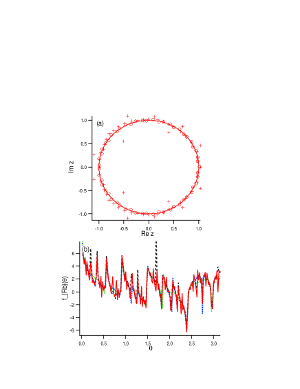
Figure 1: (Color online) (a) Distribution of poles($\bigcirc$) and zeros($+$) of the $[56|56]$ Pade approximated function for test function $f_{Fib}(z)$ with a NB on $|z|=1$. The unit circle is drawn to guide the eye. (b)The Pade approximated function $f_{Fib,r}^{[56|56]}(\theta)$, and exact function $f_{Fib,r}(\theta)$ in $\theta-$representation with $r=1.0$.

It can be expressed that the complex zeros of the polynomial (9) cluster near unit circle $|z|=1$ and the zeros distribute uniformly on the circle as $F_{N}\to\infty$ by Erdos-Turan type theorem in appendix B erdos50 ; amoroso96 ; odlyzko93 ; simon04a ; simon04b ; simon10 . Furthermore, we give other exact Pade approximated function for the other lacunary series in appendix A.

II.2.2 Example 2: Random power series

Let us examine the random power series as the second example:

$$f_{noise}(z) = \sum_{n=0}^{\infty}\epsilon r_{n}z^{n}.$$ (10)

Here the random sequence $\{r_{n}\}$ is independently and identically distributed (i.i.d.) random variable which take the value within $r_{n}\in[0,1]$, and $\epsilon$ is the strength of the randomness. It is shown that in general the noisy function has a NB on the unit circle $|z|=1$ with probability one. (See Gilewicz’s theorem in appendix B.)

Figure 2 shows distribution of poles and zeros of the $[50|50]$ Pade approximated function for $f_{noise}(z)$. The poles inside the unit circle $|z|=1$ are cancelled with zeros at a very nice precision, forming the ghost pairs. On the other hand, the poles and zeros pairs accumulated around $|z|=1$ form close pairs but are not exactly cancelled. Such close pairs are sometimes called as Froissart doublets. They approximate well the NB of the random power series on $|z|=1$.

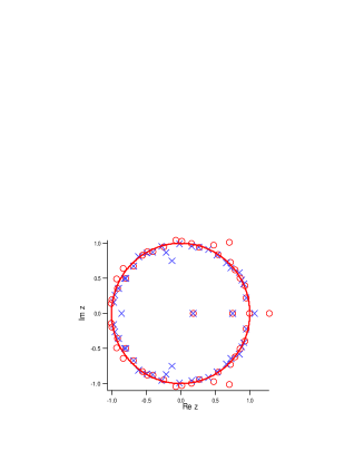
Figure 2: (Color online) Distribution of poles ($\bigcirc$) and zeros ($\times$) of Pade approximated function $f_{noise}^{[50|50]}(z)$ for a random power series $f_{noise}(z)$ with the noise strength $\epsilon=1$. The unit circle is drawn to guide the eye.

In this case, it has been often noticed that the complex zeros of the random polynomial also distribute uniformly on the unit circle $|z|=1$ as a limit $N\to\infty$. (See Erdos-Turan type theorem in appendix B.) The relation between the distribution of zeros of the polynomials with random coefficients and the pole-zero pairs distribution of the Pade approximated function is interesting and future problem.

III Detection of singularities by expansion-center-shift

In this section, we give a simple idea to investigate the singularity of the functions based on estimation of the convergence radius of power expansion about the shifted center. This numerical method can take up the slack result by the Pade approximation.

III.1 expansion-center-shift

We consider the following function $F(z)$ with convergence radius $R_{c}=1$, which is expanded about $z=0$ as follows,

$$F(z)=\sum_{n=0}^{\infty}a_{n}z^{n}.$$ (11)

Here we would like to investigate whether the circle $|z|=1$ is a NB or not. To this end, we shift the expansion center from about origin to around the $|z|=1$, and estimate the convergence of the new expansion. Then, new expansion about the center $\omega=(1-\epsilon)e^{i\phi}$ inside of the convergence domain $|z|<1$ becomes,

$$F(z)=\sum_{m=0}^{\infty}b_{m}(z-\omega)^{m},$$ (12)

where $\epsilon(<1)$ denotes the distance from the convergence edge $|z|=1$ and $\phi$ is the argument of the center. We can express the coefficients $\{b_{m}\}$ in terms of the coefficients $\{a_{n}\}$ of the truncated Taylor series Eq.(11) as follows:

$$b_{m}\equiv F^{(m)}(\omega)/m!\simeq\sum_{n=m}^{N}F_{mn},$$ (13)

where

$$F^{(m)}(\omega) = \frac{d^{m}}{dz^{m}}F(\omega),$$ (14)

$$F_{mn} = \frac{n!}{m!(n-m)!}\omega^{n-m}a_{n}.$$ (15)

The new convergence radius of the function $F(z)$ can be given by the coefficients $\{b_{m}\}$ of the center-shifted expansion as,

$$R(\omega) = \lim_{m\rightarrow\infty}R_{\omega}(m)$$ (16)

$$\equiv \lim_{m\rightarrow\infty}\frac{1}{\sqrt[m]{|b_{m}|}}.$$ (17)

Accordingly, if the convergence radius becomes $R(\omega)=\epsilon$ for any angles $\phi$ of deviation when the center $\omega$ of the expansion is shifted close to the circle $|z|=1$ from its inside, we can guess the unit circle $|z|=1$ is the NB of the function. (See Fig.3.) We will call this direct method of searching for the singularities as ”expansion-center-shift”.

In appendix C, we give some technical remarks when we numerically apply the expansion-center-shift.

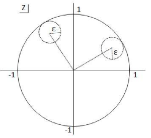
Figure 3: (Color online) Illustration of expansion-center-shift to confirm the existence of natural boundary on $|z|=1$. $\epsilon$ is the distance between the center $\omega$ of the expansion and the unit circle $|z|=1$.

III.2 Application of the expansion-center-shift to functions with poles and NB

Here, we give some numerical examples to which the expansion-center-shift is applied. In the case of lacunary series the nonzero expansion coefficients become more and more sparse with increase in the order of expansion, and thus it does not afford significant numerical result for the expansion-center-shift.

III.2.1 Example 1: artificially constructed functions with poles

As a first example we consider the following artificially constructed functions with some poles on the circle $|z|=1$ as,

$$f_{pole}(z)=\sum_{k}\frac{1}{z-z_{k}},$$ (18)

where $z_{k}={\rm exp}{i\theta_{k}}$.

Figure 4 shows the $m-$dependence of the convergence radius given by (16) for $f_{pole}(z)$ with poles at $z_{0}=1$, $z_{\pm 1}={\rm exp}\{\pm i\pi/8\}$. It is found that the convergence radius $R$ smoothly converges to $\epsilon$ when the location of the center $\omega$ of expansion is on the real axis, i.e. $\phi=0$, as seen in Figure 4(a). On the other hand, Figure 4(b) shows the convergence radius $R(m)$ as a function of $m$ when the arguments of the expansion center are taken as $\phi=0,\pi/32,\pi/16,\pi/8$ at a fixed $\epsilon=0.1$. As is expected, it asymptotically converge to the the distance between the expansion center $\omega$ and the location of the nearest pole. The distances are $0.1,0.137,0.211,0.1$ for $\phi=0,\pi/32,\pi/16,\pi/8$, respectively.

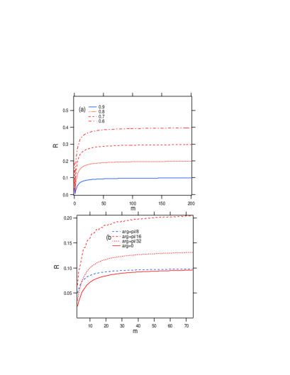
Figure 4: (Color online) Convergence property of $R(m)$ for an artificially constructed function $f_{pole}(z)$ with the poles at $z_{0}=1$, $z_{\pm 1}={\rm exp}\{\pm i\pi/8\}$. (a)The cases of the radius $\epsilon=0.4,0.3,0.2,0.1$ at a fixed $\phi=0$. (b)The cases of the argument $\phi=0,\pi/32,\pi/16,\pi/8$ at a fixed $\epsilon=0.1$.

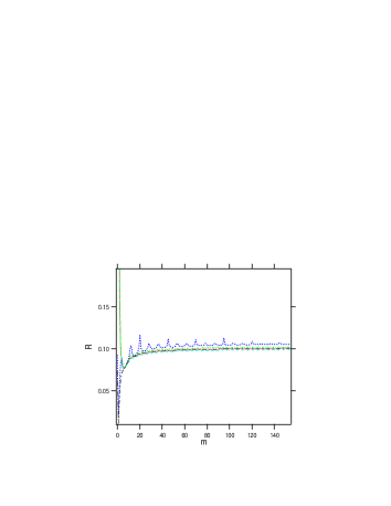
Figure 5: (Color online) Convergence property of $R(m)$ for the an artificially constructed function $f_{pole}(z)$ with 80 poles symmetrically distributed with a regular interval on the unit circle $|z|=1$. These results are shown for five randomly chosen arguments $\phi$ within $[0,\pi/4]$ and $\epsilon=0.1$.

Figure 5 shows the results for an artificially constructed function with 80 poles symmetrically distributed on the unit circle $|z|=1$. The convergence radius approach the value $\epsilon$ regardless of the argument $\phi$ of the expansion center. The fluctuation is cancelled due to superposition of the contribution from the many poles in the almost all cases.

As a result, the expansion-center-shift can numerically detect the singularities of the functions with poles on the unit circle $|z|=1$.

III.2.2 Example 2: Random power series

As a second example, let us apply the expansion-center-shift for the random power series which has a NB on the unit circle $|z|=1$ with probability 1.

Figure 6 shows the the variation $R(m)=|b_{m}|^{-1/m}$(Eq.(16)), at 6 different arguments of the expansion center taking $\epsilon=0.2$ and $\epsilon=0.1$. $R(m)$ converges to $\epsilon=1-|w|$ for all angles, which is consistent with the fact that $|z|=1$ is the NB.

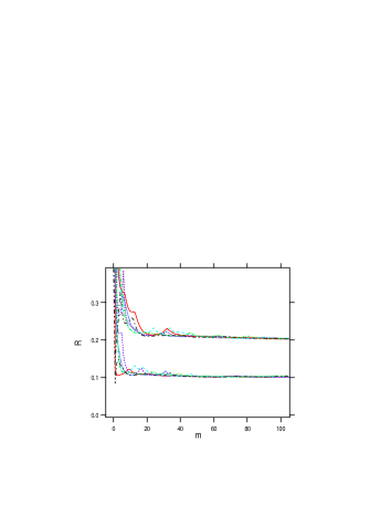
Figure 6: (Color online) Convergence property of $R(m)$ for the random power series. These results are $N=2000$ and $\epsilon=0.1,0.2$ for 6 different some arguments.

At the end, we list up some noteworthy facts when we use the expansion-center-shift: (i) it is applicable to detect singularity on a circle $|z|=1$ by using the rescaled expansion coefficients $\{a_{n}\}$ of order $O(1)$. (ii)it is a complementary method for Pade approximation which suggests the location of the singularity by the distribution of the poles and zeros around on $|z|=1$.

IV Analyticity of some quantum states I:Pade Approximation

In the following two sections, it will be shown that NB of the quantum wavefunctions can be numerically detected by Pade approximation and expansion-center-shift. In this section, we investigate the singularity of wavefunction by Pade approximation. To our best knowledge, this is the first attempt to characterize the singularity of wavefunction in the complex plane.

IV.1 Basic setting

We investigate the eigenstates of one-dimensional tight-binding model in the site representation of Shr$\ddot{o}$dinger equation $H|\Psi>=E|\Psi>$ a typical quantum states $\{u(n)\}$,

$$u(n-1)+u(n+1)+V_{n}u(n)=Eu(n),$$ (19)

where $u(n)=<n|\Psi>$, and $E$ and $V_{n}$ are energy of the system and the on-site energy, respectively. In this paper, fixed boundary condition, $u(0)=u(N)=0$, is used in order to make the all the amplitudes $\{u(n)\}$ real values, for simplicity. Here, $N$ denotes the system size. The following expression by the transfer matrix $T_{n}$ is sometime convenient.

$$\left(\begin{array}[]{c}u(n+1)\\ u(n)\\ \end{array}\right)=T_{n}\left(\begin{array}[]{c}u(n)\\ u(n-1)\\ \end{array}\right),$$ (24)

where

$$T_{n}=\left(\begin{array}[]{cc}E-V_{n}&-1\\ 1&0\\ \end{array}\right).$$ (27)

The Lyapunov exponent (Landauer exponent) is then defined in the thermodynamic limit $N\to\infty$ as,

$$\gamma=\lim_{N\to\infty}\frac{\log\parallel\prod^{N}_{n=1}T_{n}\parallel}{2N},$$ (28)

where $\parallel.\parallel$ is a matrix norm. The localization length $\xi$ is given by $\xi=1/\gamma$. This growth is also related to growth/decay properties of generalized eigenfunctions associated with the Schrodinger equation.

The Fourier representation of the eigenstate $u(n)$ is given as,

$$\Psi(p)=\frac{1}{\sqrt{N}}\sum_{n=1}^{N}e^{-ipn}u(n),$$ (29)

where $p=2\pi P/N,P=0,1,...,N-1$. It converges to an analytic function of continuous real variable $p$ by taking the limit $N\to\infty$ if the series $u(n)$ has a finite radius of convergence numerically. (A concrete example of convergence in the limit $N\to\infty$ is demonstrated for Harper model in Fig.8.) Moreover, we can straightforwardly extend the real continuous function $\Psi(p)$ by taking the limit $N\to\infty$ into the complex plane and shifting $p\to p+i\eta$, where $\eta(>0)$ is a real variable.

Before that, we consider $\Psi(p+i\eta)$ when the eigenfunction $\{u(n)\}$ is exponentially localized around a center of the localization $n_{0}(=0)$ in the lattice space.

$$\Psi(p+i\eta)=\frac{1}{\sqrt{N}}\sum_{n=-N_{L}}^{N_{R}}{\rm e}^{-inp}{\rm e}^{\eta n}u(n),$$ (30)

where $N_{L}$ and $N_{R}$ denote the left- and right-extremity of the lattice space, respectively. ($N=N_{L}+N_{R}$ and $N_{L}=N_{R}$ in our case.) We introduce a complex variable $z$ given by

$$z\equiv{\rm e}^{-ip}{\rm e}^{\eta}={\rm e}^{-i(p+i\eta)},$$ (31)

and divide the function $\Psi(z)$ into two parts as follows,

$$\Psi(z) = \Psi_{+}(z)+\Psi_{-}(z),$$ (32)

$$\Psi_{+}(z) = \frac{1}{\sqrt{N}}\sum_{n=0}^{N_{R}}z^{n}u(n),$$ (33)

$$\Psi_{-}(z) = \frac{1}{\sqrt{N}}\sum_{n=-1}^{-N_{L}}z^{n}u(n).$$ (34)

Here, $\Psi_{-}(z)$ is analytic in p-axis because the factor $e^{\eta n}$ works as the convergence factor for $n<0$, and the singularity of the quantum state $\Psi(z)$ comes from $\Psi_{+}(z)$.

In general, we have to use the expansion coefficients with the order $O(1)$ to keep the numerical accuracy of Pade approximation as far as possible, and to make the radius of convergence in order $O(1)$. Accordingly, we should apply Pade approximation to $\Psi_{+}(z)$ by using the rescaled coefficients $\{u(n)e^{\gamma n}\}$ of the exponentially localized quantum state and the rescaled variable $z/e^{\gamma}\to z$ in Eq.(30) where $\gamma$ is the Lyapunov exponent of the localized state.

IV.2 Impurity states

First of all, we examine the impurity localized states which is obtained by changing the value of the on-site energy at only two adjacent sites to different value from the other sites in the tight-binding model. Generally, the impurity problem can be exactly solved and the localized state decay exponentially from the localized center at the impurity site to the outward. (See Fig.7(a).) In this case, we used the amplitude $\{u(n)\}$ without the scaling by the exponential factor because it is particularly useful for distinguishing the true pole on real axis from the ghost ones around $|z|=1$ as shown below.

Figure 7(b) and (c) show the distribution of the pole-zero pairs of the diagonal Pade approximated function for the impurity localized states. There are poles inside and outside of the unit circle $|z|=1$. It follows that all zero-pole pairs are canceled with each other making ghost zero-pole pairs except for an isolated pole (and an isolated zero) on the real axis. The location of the true poles are stable for changing the order of the Pade approximation. Apparently, the impurity state with exponential localization can be characterized by a simple pole-type singularity in the Pade approximation. The distance of the isolated true pole from the origin gives the localization length of the impurity state.

@

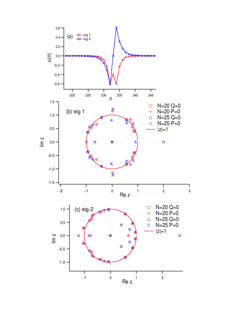
Figure 7: (Color online) Pade approximation for impurity localized states. (a)Typical symmetric impurity localized states($eig1$) and the anti-symmetric one($eig2$). (b),(c)Distribution of poles ($\bigcirc,\bigtriangleup$) and zeros ($+,\times$) of $[20|20]$ and $[25|25]$ Pade approximations for the two donor type impurity states. The unit circle is drawn to guide the eye.

IV.3 Localized states of Harper model

In this subsection, we apply Pade approximation to the localized eigenfunction of Harper model, in which the sequence of the on-site energy oscillates as $V_{n}=2V\cos(2\pi\alpha n)$ in the tight-binding model Eq.(19), where $\alpha$ is an irrational number, and $V$ is the potential strength. Due to the oscillation of on-site potential incommensurate with the lattice site all of the eigenstates are exponentially localized for $V>1$, but they are extended for $V<1$. The localization length is given by $1/\ln|V|(=\gamma^{-1})$ for $V>1$. Localization means that the eigenfunction is normalizable, ie., $\sum_{n}|u_{n}|^{2}<+\infty$. At the critical parameter value $V=1$, the eigenfunctions exhibit multifractal and their spectrum is conjectured to be singular continuous. Further, a quite interesting fact is that a diffusive motion very close to a normal diffusion is realized in the wavepacket propagation.

In general, eigenstates of the quasiperiodic systems are studied by using a rational approximation of the irrational number. Here we used Fibonacci rational approximation for the golden mean as $\alpha=F_{m-1}/F_{m}$. In practice, Fig 8 shows the discrete Fourier series expansion $\Psi(p)$ of the localized eigenstates of Harper model for three-different system size $N$. It is found that the Fourier series expansion $\Psi(p)$ of the localized state converges a continuous function with self-similar fluctuation in a limit $m\to\infty$ of the Fibonacci approximation.

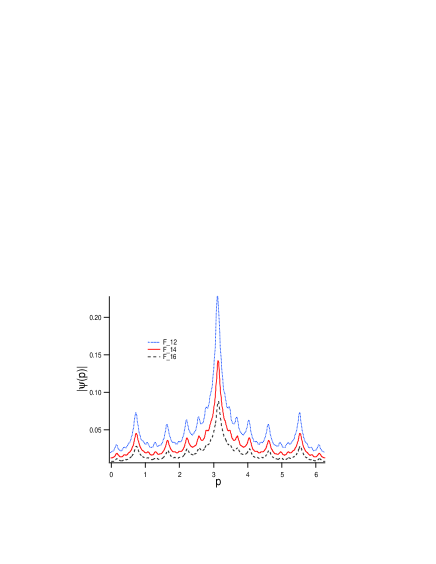
Figure 8: (Color online) The absolute value of the Fourier transformation $|\Psi(p)|$ of a localized state ($V=1.05$) of Harper model. All eigenfunctions are symmetric or antisymmetric because we set the system symmetric configuration the in the lattice space. The results are shown for $N=2F_{12}$, $N=2F_{14}$, $N=2F_{16}$. The ground states are used in each case for simplicity.

For $|z|<1$ the series $\Psi_{+}(z)$ converges absolutely and the limit $N\to\infty$ can be taken without any problem. Accordingly, in the numerical approach for the localized states, we can expect that the $\Psi_{+}(p)$ becomes an analytical function in a limit $N\to\infty$.

In addition, fortunately, in the case of the ground state of Harper model, the localized state continues to the critical state very smoothly as a limit $V\to 1+$ as seen in Fig.9. Accordingly, we can conjecture that even the localized state has essentially the same multifractal singular structure as the critical state if the exponential decaying factor is eliminated, which means to observe the localized state at the border of the analytic domain in the complex plane.

This observation motivates us to investigate the analyticity of a function $\Psi_{+}(z)=\sum_{n}s_{n}z^{n}$ of the localized eigenstates by using the scaled amplitude $s(n)=u(n)e^{\gamma|n|}$ for the eigenstate.

Note that, as mentioned in the last subsection, the factor $e^{-|n|\gamma}$ works as the convergence factor of the series $\sum_{n}u_{n}z^{n}$, and the Lyapunov exponent $\gamma$ corresponds to the depth $\eta$ of the analytic domain of the $\Psi_{+}(p)$ in the complex $p-$plane. As a result, we can directly study complicated fluctuation of the eigenstates by the rescaling procedure, which are associated with the singularity ketoja95 .

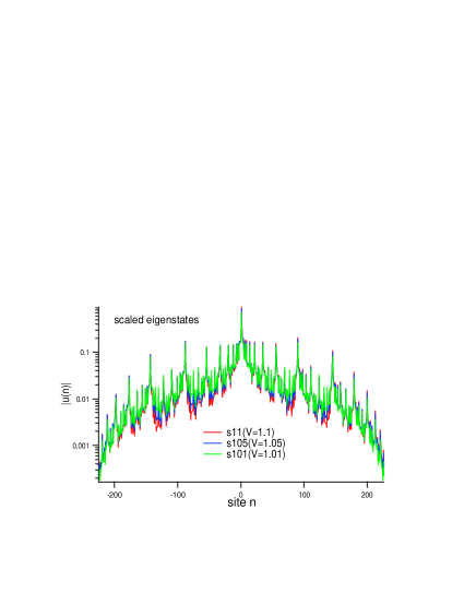
Figure 9: (Color online) The eigenstates scaled by the Lyapunov exponent $\gamma$, inverse localization length, of the Harper model with $V=1.1,1.05,1.01$. The ground states are used in each case.

We apply Pade approximation to the localized eigenstate of Harper model, where the ground state of Harper model with $V=1.1$ is taken as a typical example. As are seen in Fig.10 and Fig.11, the all zero-pole pairs are perfectly cancelled inside the circle $|z|<1$ , on the other hand, around $|z|=1$ and outside the circle the pairs are not cancelled. The distribution of the poles tend to cluster around $|z|=1$, which strongly suggests that $|z|=1$ is a NB as $N\to\infty$.

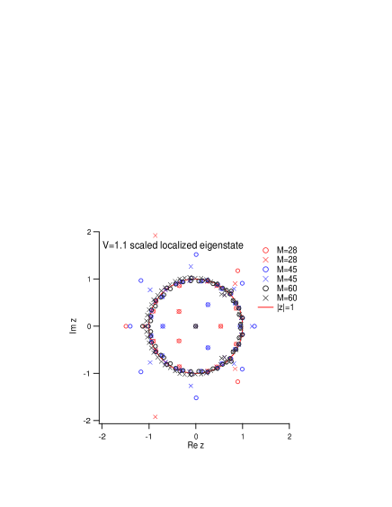
Figure 10: (Color online) Distribution of poles ($\bigcirc$) and zeros ($\times$) of the $[28|28],[45|45]$ and $[60|60]$ Pade approximations for the scaled localized state ($V=1.1$). The result is for the eigenstate in Fig.9. The unit circle is drawn to guide the eye.

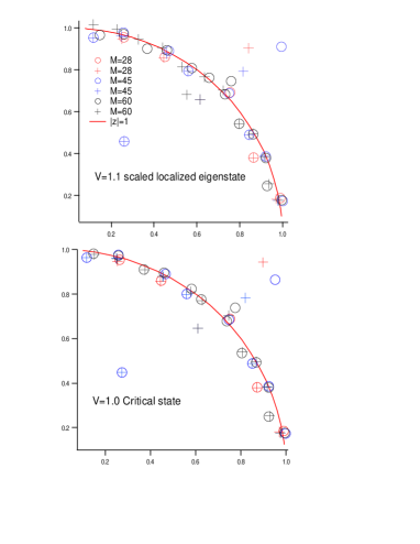
Figure 11: (Color online) (a)An expansion of Fig.10 and (b)the critical state($V=1.0$) of Harper model.

Figure 12 shows Pade approximated eigenfunctions and the exact eigenfunctions in the $\theta-$representation $\Phi_{r}(\theta)=\Phi(r{\rm e}^{i\theta})$ for the eigenstate of the Harper model with $V=1.1$. The similar result holds for the critical state because the shape of the scaled wavefunction of the localized state is almost similar to the critical state. The peak structures of the critical state and of the localized state almost coincide with each other even on the unit circle $|z|=1$($r=1$), and they perfectly coincide in the case of the $r=0.98$, which is very little inside the unit circle. These results strongly suggest that the localized ground state of Harper model has a NB on $|z|=1$ irrespective of the value of $V$ when we rescale the variable by the Lyapunov exponent. However, we should pay an attention to the following facts in the Harper model. (a)All the eigenstates have same localization length if the potential strength $V$ is same. (b)In the localization cases ($V>1$) the eigenstates rescaled by the Lyapunov exponent have the similar structure as the corresponding critical state ($V=1$), regardless of the potential strength. (c)The most important feature is self-dual at the potential strength $V=1$ (Aubry duality): the equation for the Fourier transform $\Psi(p)$ of $u(n)$ is identical to Eq.(19). The quantum eigenstates are extended for $V<1$, exponentially localized for $V>1$ and at the critical value $V=1$, the states are power-law localized. Accordingly, all claims for $V>1$ hold for the cases of $V<1$ in the conjugate representation.

As a result, we can expect that all the eigenstates of Harper model have a NB on $|z|=1$ in the limit $N\to\infty$ if we rescale by the Lyapunov exponent and transform the eigenfunctions. The scaling by the Lyapunov exponent ($\gamma\to 1/\log V$) is equivalent to elimination of the exponential factor from the amplitude of the eigenfunctions and to access to the convergence of radius of the series $\Psi(p)$.

Thus the complex structure of wavefunction observed on the real space only at the critical value $V=1$, which yields a normal diffusion that is seemingly a time-irreversible dynamics. However, the structure potentially exists in the complex plane as the NB even in the localized states with $V$ larger than the critical value.

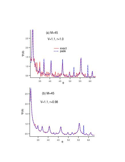
Figure 12: (Color online) Comparison of exact and the $[45|45]$ Pade approximated eigenstates in $\theta-$representation $\Psi_{r}(\theta)\equiv\Psi(r{\rm e}^{i\theta})$ fixed at (a)$r=|z|=1.0$, (b)$r=|z|=0.98$. Here the ground state of Harper model with $V=1.1$ is used.

Finally we would like to point out that the rescaled localized states $s(n)$ satisfies the following equation,

$$e^{-\gamma}s(n+1)+V_{n}s(n)+e^{\gamma}s(n-1)=Es(n).$$ (35)

Ketoja and Satija have directly investigated the fluctuation of the eigenstate of the scaled Harper equation. ketoja95 ; satija99 ; Jazaeri01 . This is nothing more than the eigenstates in non-Hermitian Harper model hatano96 .

IV.4 Anderson-localized states

The localized states of Harper model, as well as the Bloch states and the impurity states, are specific in the sense that the on-site energy follows an artificially constructed simple sequence. In this subsection, we deal with Anderson model that describes a more natural random systems with a statistically translational invariance.

All the eigenstates are exponentially localized when the sequence of the on-site energies $\{V_{n}\}$ are generated by i.i.d. random variables in the tight-binding model in Eq.(19). We take uniform distribution $V_{n}\in[-W,W]$, where $W$ denotes the disorder strength. Furstenberg’s convergence theorem on the product of matrices in Eq.(28) ensure the positive definite value of the Lyapunov exponent:

$$Prob(\gamma>0)=1,$$ (36)

with probability 1 for almost every energy if $\{V_{n}\}$ are i.i.d. random variables.

Let us apply the Pade approximation to a typical Anderson-localized state with exponential decay decorated by complicated fluctuation, as seen in Fig.13(a). Note that it is a typical double-hump state with two exponential peaks mott70 . Here we rescale an exponential decay part of the double-hump state with shape of two exponential peaks in Fig.13(b) and (c) by the numerically estimated Lyapunov exponent, and apply the Pade approximation for the rescaled state.

Figure 14(a) shows the pole-zero pairs of Pade approximation for the typical Anderson-localized state. All pole-zero pairs are cancelled inside the circle $|z|=1$ as is the case of the impurity localized state in Fig.7. However, it follows that in the Anderson-localized state some poles around the unit circle remains, and they are not canceled with zeros. The distribution of poles and zeroes seems to suggest the existence of the NB on $|z|=1$, but we can not give a definite conclusion. This is because, unlike Harper model, the fluctuation around the exponential decay of localized wavefunction is so wild that it mask the systematic decay within the number of sites available for finite-order Pade approximation. The suggestion, however, can be strongly supported by the complementary analysis in Sect. V and some considerations in Sect.VI.

As have been done for the simple examples with a NB in Sect.II and also for the Harper model in the last subsection, we confirmed the validity of Pade approximation by comparing the Pade-approximated eigenfunction with the original eigenfunction in the angle representation. Figure 14(b) shows the Pade approximated function can well reproduce the corresponding part of the original eigenfunction.

Generally, Pade approximation become less accurate with the decrease in the order of the approximation. In particular, it is less reliable when the sign of the coefficient fluctuates very wildly as is the case of the Anderson-localized states. Accordingly, it is rather difficult to distinguish the type of the singularity (finite many simple poles or NB) only by Pade approximation whose order is very limited. (See Fig.14(b))

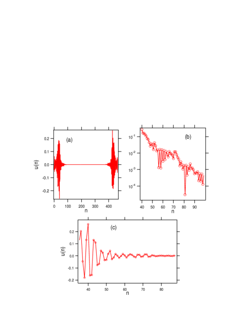
Figure 13: (Color online) (a)A typical ${u(n)}$ of Anderson-localized state at band edge in the Anderson model with $N=512$ and $W=1$. (b)A part of the exponentially localized state $|u(n)|$ in the semi-logarithmic scale. (c)A part of the amplitude of the localized state used in Pade approximation.

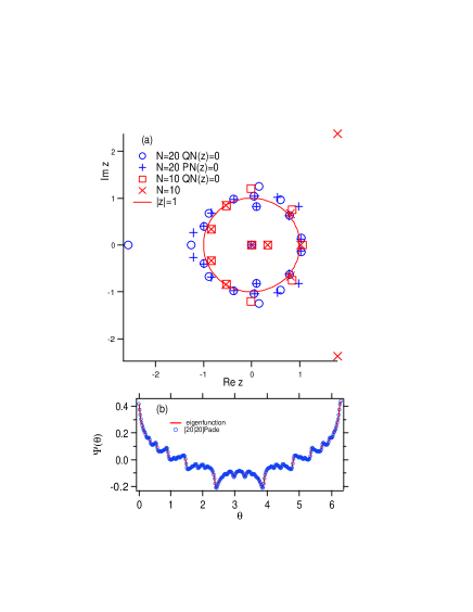
Figure 14: (Color online) (a)Distribution of poles ($\bigcirc,\Box$) and zeros ($+,\times$) of the $[10|10]$ and $[20|20]$ Pade approximated functions for the localized eigenstate. The unit circle is drawn to guide the eye. (b)The $[20|20]$ Pade approximated functions and the original wavefunction in $\theta-$representation with $r=1.0$. Note that only a part of the eigenstate used in the Pade approximation is shown.

Before closing this subsection, we comment on the fluctuation of the wavefunctions. Multifractal analysis of the fluctuations of Anderson-localized eigenstates in the one-dimensional disordered model shows multifractality of the rescaled eigenstates by the exponential factor pietronero87 . The scaled eigenstates have multifractal property in both inside and outside localization length.

It is natural to suppose that such a complicated fluctuation is due to the NB of the Anderson-localized states in the $p-$representation. However, unlike the Harper model, it is difficult to give a more accurate proof by a theoretical technique such as renormalization procedure, as shown in the last subsection.

V Analyticity of some quantum states II: expansion-center-shift

In this section, we apply the expansion-center-shift to the quantum eigenstates to strengthen our claim in the last section that the quantum localized states have a NB. In this method, much higher-order expansion coefficients than the Pade approximation are necessary to get accurate results.

V.1 Impurity states

First of all, we apply the expansion-center-shift to the impurity state rescaled by the numerically estimated exponential factor. Therefore, it is convincible that the impurity state is characterized by a simple isolated pole on the real axis based on a result of Pade approximation in the last section.

Figure 15(a) shows the results for the cases of the expansion centers being shifted to $\omega(=1-\epsilon)=0.8,~{}0.9$ on the real axis, i.e. the argument $\phi=0$. They are shown by solid lines for donor type impurity state and by dashed lines for accepter type impurity state, respectively. It is found that in the case of acceptor type impurity state the convergence of $R(m)=1/\sqrt[m]{|b_{m}|}$ is slower than that of donor type impurity state due to the alternating sign of the amplitude. Note that the acceptor impurity state is oscillatory localized with the same localization length as the donor impurity state. In all cases, the radius $R(m)$ converge to the expected value as $m$ increases. A convergence problem as seen in Sect.III does not occur in this case.

Next, fixing $1-|w|=\epsilon=0.1$, we examined the convergence property by changing the argument $\phi$ (arg$w$) for the donor type impurity state. As shown in Fig.15(b), $R$ converges well to the expected value in each case based on assumption that a simple pole is located at $z=1$. (Note that we used the rescaled impurity eigenstate.) In this case the convergence problem for larger $m$ comes up with increase value of the argument $\phi$, as we discussed in Sect.III and appendix C.

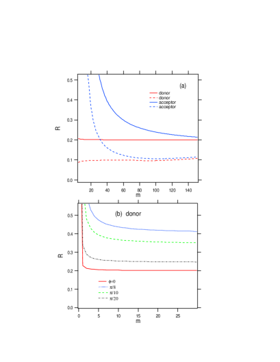
Figure 15: (Color online) Convergence property of $R(m)$ for the impurity states rescaled by exponential factor. (a)The cases of the $\epsilon=0.2,0.1$ with $\phi=0$ and (b)the cases of the argument $\phi=0,\pi/32,\pi/16,\pi/8$ with $\epsilon=0.1$ are shown.

As a result, the expansion-center-shift suggests that the impurity states can be characterized by simple pole at real axis that is consistent with the result by Pade approximation in the last section.

V.2 Localized eigenstates of Harper model

We will reexamine whether the unit circle $|z|=1$ is a NB of the localized state of Harper model ($V=1.02$) by the expansion-center-shift. We use the rescaled expansion coefficient $s(n)={\rm exp}(\gamma|n-n_{0}|)u(n)$ as in the Pade approximation, where $\gamma(=1/\log V)$ is the Lyapunov exponent and $n_{0}$ is a localization center of the localized state.

The convergence property is shown in Fig.16 by taking $|w|-1=\epsilon=0.2$ and $\epsilon=0.1$ for various values of $\phi={\rm}argw$. For all values of $\phi$ the $R(m)$ converges to the expected values, namely, $R(m)\to 0.2$ for $\epsilon=0.2$ and $R(m)\to 0.1$ for $\epsilon=0.1$, respectively. This fact means that at any point on $|w|=1-\epsilon$ the power series expansion of the wavefunction has the convergence radius $\epsilon$, and the singularities are densely distributed on $|z|=1$. The result suggests the unit circle is a NB of the localized eigenstates of Harper model.

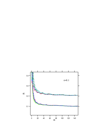
Figure 16: (Color online) Convergence property of $R(m)$ for the scaled localized state of Harper model ($V=1.02$). These results are shown for $N=2F_{16}=1974$ and $\epsilon=0.1,0.2$ with randomly selected 10 arguments of the expansion center.

V.3 Anderson-Localized eigenstates

Figure 17 shows a typical Anderson-localized state around the band center. The exponentially decaying part used in the expansion-center-shift is also shown. We take the rescaled amplitude $s(n)={\rm exp}(\gamma|n-n_{0}|)u(n)$ of the localized states, where $\gamma$ is the numerically estimated Lyapunov exponent of the localized eigenstate. As mentioned in Sect.III, we estimate the convergence radius $R(m)$ of the center-shifted power series about $w=(1-\epsilon){\rm e}^{i\theta}$. The convergence property is shown in Fig.18 for $\epsilon=0.1$ and many different arguments of the expansion center. The convergence of radius of new expansion about the center $\omega$ vicinity of $|z|=1$ strongly suggests the unit circle is a NB of the rescaled eigenstates as is conjectured by the Pade approximation.

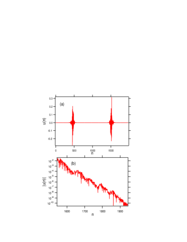
Figure 17: (Color online) (a)A typical Anderson-localized state $\{u(n)\}$ around the band center in the Anderson model with $N=2000$ and $W=1$. (b)A part of the exponentially localized state $|u(n)|$ in the semi-logarithmic scale used in the expansion-center-shift.

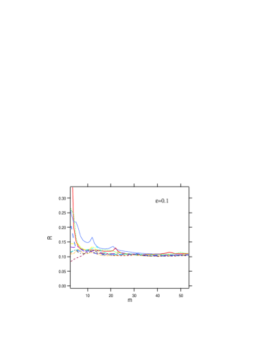
Figure 18: (Color online) Convergence property of $R(m)$ for the rescaled Anderson-localized state in Fig.17. These results are shown for $W=1$, $N=2000$ and $\epsilon=0.1$ for the expansion-center-shift with randomly selected 10 arguments of the expansion center.

VI Localized quantum states and NB of the potential

In this section, we discuss about an interesting relation between analyticity of the potential $V_{n}$ of one-dimensional tight-binding model and the eigenfunctions based on recently proved mathematical theorems. By the analyticity of potential $V_{n}$ we means the analyticity of the $Z-$transform $V(z)=\sum_{n}V_{n}z^{n}$, namely, the momentum representation of the potential function if we take $z={\rm e}^{-ip}$. We refer to $V(z)$ as the potential generating function (PGF) in the present paper.

G-M-P theorem goldsheid77 states that one-dimensional Schrodinger equation with an ergodic and stationary random potential have a positive Lyapunov exponent ($\gamma>0$) of the wavefunction with probability 1. The positive Lyapunov exponent is necessary-sufficient condition for a pure point set spectrum of the operator and all the eigenfunctions decay exponentially at $n\pm\infty$. For the random $V_{n}$ its PGF has a NB according to the Steinhaus’s theorem, and thus the presence of the pure point spectrum of random Schrodinger equation corresponds to the existence of the NB of PGF the random series. Recently, Breuer and Simon discovered a more general correspondence between the analyticity of PGF and the spectral property of the Schrodinger operators breuer11 .

Theorem 1a (Breuer-Simon 2011): Let $a_{n}(\omega)$ be a stationary, ergodic, bounded, nondeterministic process. Then for a.e. $\omega$, $f(z)=\sum_{n=0}^{\infty}a_{n}z^{n}$ has a strong NB.

On the other hand, in the localization problem of one-dimensional continuous/discrete Shrodinger operators, Kotani theory and its extended versions kotani82 ; simon83 ; kotani86 show more powerful results than G-M-P theorem.

Theorem 1b (Kotani 1982): If the potential sequence $V_{n}$ is nondeterministic under the conditions (i)stationarity, (ii)ergodicity, (iii)integrability, then there is no absolutely continuous (a.c.) spectrum of the operator.

The stationarity means a translation invariance of the sequence, and integrability is the boundedness of the ensemble average. And the stationarity and ergodicity ensure Kolmogorov $0-1$ law. In the Kotani’s meaning, roughly speaking, the non-deterministic potential sequence means that left-half part of the sequence can not determine whole of the right-half part of the sequence a.e. with respect to the probability measure.

Note that these conditions for the potential sequence is much weaker than the stationary random potential condition of the localization. Indeed, it will be the weakest sufficient condition for the occurrence of the weak localization (weak localization means there is no a.c. spectrum), and it is quite interesting that these conditions for the weak localization supports the presence of the NB of the PGF.

The above pair of theorems suggests that there is an interesting parallelism between the two properties that the potential has a NB and that the potential yields the weak localization.

An another pair of theorems implying this parallelism is for an apparently deterministic incommensurate potential with discontinuities,

Theorem 2a (Damanik-Killip 2005)damanik04 : Consider the tight-binding model with $V_{n}(\theta)=g(\alpha n+\theta)$, where $\alpha$ is irrational, g is bounded and periodic with period 1, and $g(z)\in[0,1]$. $g(z)$ is continuous except at finitely many points, at one of which it has different right and left limit. Then for a.e. $\theta$, the tight-binding model has no a.c. spectrum.

Theorem 2b (Breuer-Simon 2011): Let a function $g(z)$ be as in the Damanik-Killip. Then for all $\theta$, $f(z)=\sum_{n=0}^{\infty}g(\alpha n+\theta)z^{n}$ has a strong NB on $|z|=1$.

If we agree our assertion that the localized eigenstate has a NB is generally correct, then the parallelism holds for the two properties that the PGF has a NB and that the eigenfunction has a NB.

Note that the parallelism is only hold for the sufficient condition yielding the existence of NB and the occurrence of the weak localization. However, we emphasize that it is not exactly correct that whether the PGF has a NB or not respectively correspond to the localization or non-localization. Indeed, the Harper equation has a deterministic, analytic and incommensurate potential, and its PGF has no NB, but the Harper equation has localized eigenstates if the potential strength is large enough. Furthermore, there is another example. Suppose that the potential series is a lacunary series, then its PGF has a NB, but the corresponding sparse potential sequence $V_{n}$ consists of $\{0,1\}$, where the ”0” corresponds to “gap” of the series, and the Lyapunov exponent $\gamma$ of the Schrodinger operator become zero because the mean gap length becomes infinite in the limit $N\to\infty$. As a result, the spectrum is absolutely continuous and the eigenstates are extended, although the PGF has a NB. (Note that the result is not contradict with Kotani theory because the lacunary system is deterministic and nonstationary.)

In spite of the counter examples given above, the parallelism discovered by Breuer and Simon combined with our result for localized eigenstates seems to suggest that the presence of the NB in PGF and the presence of the NB in eigenstate are strongly correlated. It may be conjectured that if the PGF has a NB then at least its eigenfunction also has a NB.

VII Summary and Discussion

To investigate the very origin of complex quantum dynamics, we studied the analytical property of wavefunction in the quantum system by complexifying the argument of the eigenstates, taking one-dimensional tight-binding models, whose eigenstates exhibit exponential localization as an example.

To capture the singularities of the quantum states we investigated usefulness of the Pade approximation and expansion-center-shift for some known functions which have been proven to have a natural boundary (NB). The poles and zeros of Pade approximation accumulate around the NB with increase in order of the Pade approximation. The expansion-center-shift compensates for Pade approximation by detecting the change of convergence radius with shifting the center of power series expansion.

We used Pade approximation baker75 ; baker96 as a numerical method to investigate the properties of singularities of Fourier series (or the Z-transformation) of the localized and critical states of Harper model in comparison with the other quantum states such as impurity state and Anderson localized state. The impurity states can be characterized by simple poles of the Pade approximation. It is found that in the localized states of Anderson model and Harper model the poles and zeros of the Pade approximated function tend to cluster, forming a NB. Next, we confirmed the conclusions obtained by the Pade approximation are consistent with the result of expansion-center-shift.

Here, we discuss our original interest on quantum dynamics. It is by no means a trivial problem whether the same analytical properties as the eigenfunctions can be observed also for the time-dependent wavefunction. If the initial wavefunction is an entire function like Gaussian wavepacket, then the time-evolved wavefunction is also an entire-function for a finite time evolution. We know, on the other hand, empirically that the wavepacket is also exponentially localized in a limit of long time-evolution, and the exponential region spreads in time. As long as we focus on the exponential-decay region, as is shown in appendix D, the wavefunction practically looks as if it has a NB in a similar way to the localized eigenfunctions.

What is physical meaning of the NB of the localized eigenstates and the dynamically localized states in Anderson and Harper models?

We consider the problem based on the localized state of the Harper model. Let us consider the analytic continued eigenfunction $\Psi(z)$ of Harper model, where $z={\rm e}^{-i(p+i\eta)}$ is a complex variable. The essential structure of $\Psi(z)$ on the NB is independent of the potential strength $V$, and thus it does not depend on the localization length, and it is the same as the critical state if we rescale as $z{\rm e}^{-\gamma}\to z$ by the Lyapunov exponent $\gamma$.

Therefore, we can expect that at the NB the same phenomenon as the critical state takes place. As $V$ deceases and approaches to the critical state $V=1$, the NB goes down to the real axis, and the real axis itself become a NB. The diffusive behavior occurring in the complex space can be observed in the real world. Inversely speaking, it may be claimed that a diffusive behavior of the wavepacket would be realized already in the complex plane even for $V>1$, in other words, the localized state is a pre-diffusive state in the sense that it actually exhibits a diffusive motion in the complex plane.

With the above scenario in mind we try to go one-step further. Then we can expect that the similar scenario would hold true with the Anderson-localized states in disordered systems. Actually, Anderson-localized states have a NB and the fluctuation of the states show multifractal structure when the exponential factor is removed by the scaling of the localization length. Accordingly, the multifractal structure of the wavefunction is strongly related to the NB. The complex structure of eigenstates can be generated by an accumulation of the interference effect of the multi-scattering due to the randomness of the potential. Therefore, the localization-delocalization transition observed in higher-dimensional disordered systems and multiple degrees of freedoms systems can be also interpreted as the result that NB of the wavefunction approaches the real axis; it is the onset of delocalization finally leads to a normal diffusion and irreversibility of the time-reversal property. (Note that, unlike the Harper model, the delocalization do not necessary mean the normal diffusion in the case of Anderson localization.)

Therefore, we guess that the complex wavefunction associated with the emergence of the NB might be an ultimate origin of irreversibility in quantum systems.

As we considered in Sect.VI, quantum states of spatially extended “natural systems” with stationary, ergodic and bounded potential, except for very rare example such as periodic systems, have a NB, and so it potentially exhibits the onset of irreversible phenomenon such as diffusion-like motion at the NB. Under certain conditions the NB, which is usually located in the complex domain, falls down on the real space, leading to the onset of irreversible phenomenon in the real world. Conversely, even though no time-irreversible phenomena is observed in the real space, the time-irreversibility may be observed in the complex space by “complexifying” the real coordinate which is the eigenvalue of an observable. To clarify whether our scenario described above is true or not we, of course, need an actual proof, which is remained as a future problem.

Appendix A Pade approximation of Jacobi lacunary series

In this appendix, we investigate effectiveness of Pade approximation for a lacunary series $f_{Jac}(z)=\sum_{n=0}^{\infty}z^{2^{n}}$ with a NB on $|z|=1$, which is called Jacobi lacunary series after Jacobi. Some theorems for lacunary series with a NB are given in appendix B.

The Pade approximated function exactly has the following form,

$$f^{[2^{N}]}_{Jac}(z) \sim f_{Jac}^{[2^{N-1}|2^{N-1}]}(z)$$ (37)

$$= \frac{A^{N}_{Jac}(z)}{1+\sum_{k=0}^{N-2}z^{2^{k}}-z^{2^{N-1}}},$$ (38)

where explicit form of the numerator $A^{N}_{Jac}(z)$ is given as

$$A^{N}_{Jac}(z) = z+2z^{2}$$

$$+ 2\sum_{n=2}^{N-1}z^{H_{n}}(z+z^{2}+\sum_{k=1}^{n-2}z^{H_{k+2}}),$$

where $H_{n}=2^{n-1}$.

Accordingly, the poles of the $[2^{N-1}|2^{N-1}]$ Pade approximated function are given by roots of the polynomial,

$$1+\sum_{k=0}^{N-2}z^{2^{k}}-z^{2^{N-1}}=0.$$ (40)

This is just a lacunary polynomial and the zeros are distributed uniformly on the unit circle as $N\to\infty$. In Fig.19 the numerical result of Pade approximation for $f_{Jac,r}(\theta)$ is shown. The poles and zeros are plotted for the $[64|64]$ Pade approximation in Fig.19(a). In the case of $M=64$ the poles and zeros accumulate around $|z|=1$ as increase of order of the Pade approximation. Inside the circle $|z|=1$ some cancellations of the ghost pairs appear. Figure 19(b) shows the Pade approximated functions in the $\theta-$representation. It well approximate the original one when the order of Pade approximation increases.

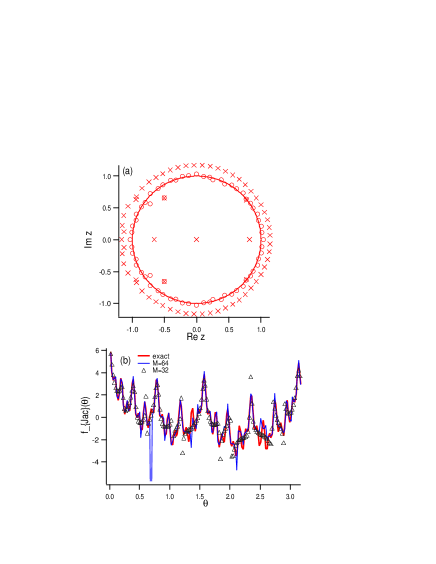
Figure 19: (Color online) (a)Distribution of poles($\bigcirc$) and zeros($\times$) of the $[64|64]$ Pade approximation for test function $f_{Jac}(z)$ with NB on $|z|=1$. The unit circle is drawn to guide the eye. (b)The Pade approximated functions $f_{Jac,r}^{[32|32]}(\theta)$, $f_{Jac,r}^{[64|64]}(\theta)$ and exact function $f_{Jac,r}(\theta)$ in the $\theta-$representation with $r=1.0$.

Appendix B Some mathematical theorems

The following theorems are well-known for function with a NB on $|z|=1$. For the details and proofs, see the references korner93 ; remmert10 .

Erdos-Turan Type theorem: Let us define a random polynomial

$$f(z)=\sum_{n=0}^{N}a_{n}z^{n},$$ (41)

where coefficients $a_{n}$ are randomly distributed and $a_{0}a_{N}\neq 0$. Then the zeros of the random polynomial cluster uniformly around the unit circle $|z|=1$ if ”size of the truncated series” $L_{N}(f)$ is small compared to the order $N$ of the polynomial, where

$$L_{N}(f)=\log\left(\frac{\sum_{n=0}^{N}|a_{n}|}{\sqrt{|a_{0}a_{N}|}}\right).$$ (42)

Note that this theorem is also hold for the polynomials with deterministic coefficients $a_{n}$ such as Newman type polynomial having coefficients in the sets $\{0,1\}$ or $\{0,\pm 1\}$.

Fabry’s gap theorem(1899): Power series

$$f(z)=\sum_{\nu=0}^{\infty}a_{\nu}z^{\lambda_{\nu}}$$ (43)

with radius of convergence $R=1$ has a NB on $|z|=1$, provided it is Fabry series, i.e.

$$\lim_{\nu\to\infty}\frac{\lambda_{\nu}}{\nu}=\infty.$$ (44)

Steinhaus’s theorem(1929): Suppose that the power series $f(z)=\sum_{n=0}^{\infty}a_{n}z^{n}$, has radius of convergence $R=1$. Let $X_{0},X_{1},...,X_{n}$ be a sequence of stochastic variables obeying i.i.d. in the interval $X_{i}\in[0,1]$. Then, with probability one, the power series

$$f_{Steinhaus}(z)=\sum_{n=0}^{\infty}a_{n}w_{n}z^{n},$$ (45)

has a NB on $|z|=1$, where $w_{k}=e^{i2\pi X_{k}}$.

Paley-Zygmund’s theorem(1932): Suppose that $r_{0},r_{1},...,r_{n},...$ be a sequence of stochastic variables taking the binary value $r_{i}=\pm 1$ with equal probability , then the power series

$$f_{P-Z}(z)=\sum_{n=0}^{\infty}r_{n}z^{n},$$ (46)

has a NB on $|z|=1$.

The similar theorem can hold for random power series $\sum_{n=0}^{\infty}r_{n}z^{n}$ with a sequence of stochastic variables obeying i.i.d. in the interval $r_{i}=[-1,1]$ and $r_{i}=[0,1]$.

Szego’s theorem (1922): Suppose that the power series $f(z)=\sum_{n=0}^{\infty}a_{n}z^{n}$, has radius of convergence $R=1$ the values of $\{a_{n}\}$ is in a finite set, then either $|z|=1$ is a NB, or else ${a_{n}}$ is eventually periodic, in which case $f(z)$ is a rational function with poles on $|z|=1$.

Notice that the condition of the potential sequence in this theorem corresponds to that in Bernoulli-Anderson model, which models alloys composed of at least two distinct types of atoms by means of the distribution of a Bernoulli random variable carmona87 ; bourgain05 .

Appendix C Some technical remarks on the expansion-center-shift

We can calculate the coefficients $\{b_{m}\}$ by the coefficients $\{a_{n}\}$ of the truncated Taylor series Eq.(11) as follows:

$$b_{m}\equiv F^{(m)}(\omega)/m!\simeq\sum_{n=m}^{N}F_{mn},$$

where

$$F_{mn}=\frac{n!}{m!(n-m)!}\omega^{n-m}a_{n}.$$ (47)

We remark some numerical problem in the evaluation of the sum (C). By using Stirling’s formula, the $n-$dependence of $F_{mn}$ is represented by

$$F_{mn}\propto\frac{n^{n}}{(n-m)^{n-m}}\omega^{n}a_{n}.$$ (48)

The modulus $|F_{mn}|$ is well approximated by a Gaussian function around $n=n_{0}$ maximizing $n^{n}/(n-m)^{n-m}|\omega|^{n}$, which gives

$$n_{0}=\frac{m}{(1-|\omega|)}=\frac{m}{\epsilon},$$ (49)

and the Gaussian approximation becomes

$$F_{mn}\sim{\rm exp}\{-\frac{\epsilon^{2}}{2m}(n-n_{0})^{2}\}(1-\epsilon)^{n}{\rm e}^{in\phi}a_{n}.$$ (50)

Thus we have to calculate a large number of coefficients $a_{n}$ such that $0\leq n\leq N$, and $n_{0}(=m/\epsilon)\gg N$ with increase in $m$ and/or decrease in $\epsilon$. In addition, even though we may prepare $a_{n}$ up to $N\gg n_{0}$, the second serious numerical problem comes from the oscillatory nature of $\omega^{n}=(1-\epsilon)^{n}{\rm e}^{in\phi}$.

Suppose the simplest and worst case $a_{n}=1$, namely $f(z)=\sum_{n}a_{n}z^{n}$ has a single pole at $z=1$, then cancellation due to the sinusoidal oscillation of $\omega^{n}$ makes the result of summation Eq.(C) extremely small as

$$\sum_{n=m}^{N}F_{mn}\sim{\rm e}^{-\frac{\phi^{2}m}{2\epsilon^{2}}},$$ (51)

except for a case $\phi=0$, which may be incomputable by numerical summation of Eq.(C) if $\epsilon$ is small and/or $m$ is large. This is the worst case, and for more general cases where $a_{n}$ has no particular regularity, things will be much relaxed. However, a particular care must be taken for the numerical accuracy of the summation.

Appendix D NB of dynamically localized wavepacket

We can expect that dynamically localized states are also have similar singularity as the localized eigenstates in Harper model and Anderson model. Therefore, by the expansion-center-shift, we confirm the idea for the dynamically localized wavepacket in Harper model numerically obtained by,

$$i\hbar\frac{\partial\Psi(n,t)}{\partial t}=\Psi(n+1,t)+\Psi(n-1,t)$$

$$+2V\cos(2\pi\alpha n)\Psi(n,t),n=1,2,...,N.$$ (52)

with initial state $\Psi(n,t=0)=\delta_{n,n_{0}}$. In the Harper model with the strength $V>1$, spread of the initially localized wavepacket is suppressed and exponentially localized by the time-evolution. Accordingly we can obtain the stable localized wavepacket after time fully elapses. (See Fig.20(a).) Here, we can factorize the exponential decay factor ${\rm e}^{-\gamma|n-n_{0}|}$ of the localized state as

$$s(n,t)={\rm e}^{\gamma|n-n_{0}|}\Psi(n,t),$$ (53)

where we can get the Lyapunov exponent $\gamma$ by numerical fitting for the dynamically localized quantum states.

We investigate the singularity of the following power series

$$F(z)=\sum_{n}Re[s(n,t)]z^{n},$$ (54)

along the unit circle $|z|=1$ by means of the expansion-center-shift, as in the main text. The expansion is constructed by the real part of the rescaled amplitude $s(n,t)$ with the order $O(1)$ of the fluctuation.(See Fig.20(b).) We can expect that the series $\sum_{n}Re[s(n,t)]z^{n}$ has a NB on $|z|=1$ due to the fluctuation as in the case of the eigenstates.

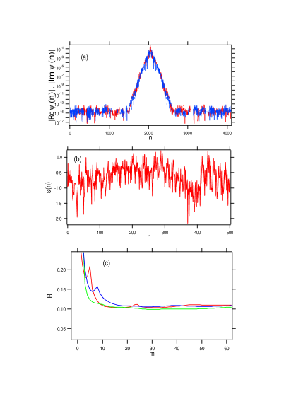
Figure 20: An exponentially localized wave packet of Harper model with $V=1.04$. (a)$|Re\Psi(t,n)|$ and $|Im\Psi(t,n)|$ of the wavepacket at $t=200$. (b)The rescaled amplitude $Re[s(t,n)]$ of the real part $Re[\Psi(t,n)]$ of 1000 sites from the localization center $n_{0}=2048$. (c)Convergence property of $R(m)$ for the rescaled localized state $Re[s(t,n)]$ of the Harper model for different three arguments. These results are shown for the system size $N=4096$ and parameters $\hbar=1$ and $\epsilon=0.1$.

Figure 20 shows the result for the dynamically localized state of the Harper model with $V=1.04$. The convergence of $R(m)$ for $\epsilon=0.1$ suggests the unit circle is a NB of the rescaled dynamically localized state. Generally, the nature of the fluctuation of the rescaled dynamically localized states $s(n)$ is not depend on the potential strength $V$, as seen in the cases of the localized eigenstates. Accordingly we can suggest that the dynamically localized quantum states of the Harper model have a NB in the complex plane.

References

- (1) Martin C. Gutzwiller, Chaos in Classical and Quantum Mechanics, (Interdisciplinary Applied Mathematics, Springer 1991).
- (2) H. Yamada and K.S. Ikeda, Phys. Lett. A 222, 76-80(1996).
- (3) H. Yamada and K.S. Ikeda, Phys. Rev. E 65, 046211-1-17(2002).
- (4) Quantum Chaos, Ed. by G.Casati and B.V.Chirikov (Cambridge Univ. Press, 1996).
- (5) P.W. Anderson, Phys. Rev. 109, 1492 (1958).
- (6) E. Abrahams, 50 Years of Anderson Localization (World Scientific Pub Co Inc., 2010).
- (7) Y. Aharonov and D. Bohm, Phys. Rev. 115, 485?491 (1959).
- (8) J.S.Bell, Speakable and Unspeakable in Quantum Mechanics, (Cambridge University Press; 2 edition 2004).
- (9) A.O. Caldeira, A.J. Leggett, Phys. Rev. A 31, 1059 (1985).
- (10) A.M. Nielsen, I.L. Chuang, Quantum Computation and Quantum Information (Cambridge University Press, 2000).
- (11) G. Casati, B. V. Chirikov, J. Ford, and F. M. Izrailev. Stochastic behavior of a quantum pendulum under periodic perturbation, Lecture Note in Physics 93, 334-352, (Springer-Verlag, Berlin, Germany, 1979).
- (12) S. Adachi, M. Toda, and K. Ikeda, Phys. Rev. Lett. 61, 659(1988).
- (13) P. A. Miller and S. Sarkar, Phys. Rev. E 60, 1542 (1999),
- (14) M. Goda, M. Azbel and H. Yamada, Int. J. Mod. Phys. B 13, 2705(1999); Physica B 296, 66(2001).
- (15) V.N. Kuzovkov, W. von Niessen, Eur. Phys. J. B 42, 529(2004).
- (16) A. Peres, Phys. Rev. A 30, 1610 (1984).
- (17) K. Shiokawa, B.L. Hu, Phys. Rev. E 52, 2497 (1995).
- (18) Thomas Gorin, Tomaz Prosen,Thomas H. Seligman, Marko Znidaric, Dynamics of Loschmidt echoes and fidelity decay, Physics Reports 435, 33-156(2006).
- (19) Ph. Jacquod, C. Petitjean, Adv. Phys. 58, 67 (2009).
- (20) H.S. Yamada and K.S. Ikeda, Phys. Rev. E 82, 060102(R)(2010); Eur. Phys. J. B 85, 41(2012).
- (21) H.S. Yamada and K.S. Ikeda, Eur. Phys. J. B 85,195(2012).
- (22) K. Ikeda, Ann. Phys. (N.Y.) 227, 1(1993).
- (23) Andrey R. Kolovsky, Phys. Rev. E 50, 3569-3576 (1994).
- (24) P.G.Harper, Proc. Phys. Soc. London, Sect. A 68, 874(1955).
- (25) Y.Last, Almost everything about the almost Mathieu operator I, pp366-372, in XIth International Congress of Mathematical Physics, Ed. by D.Iagolnitzer, (International Press Inc. 1995).
- (26) S.Y.Jitomirskaya, Almost everything about the almost Mathieu operator II, pp373-382, in XIth International Congress of Mathematical Physics, Ed. by D.Iagolnitzer, (International Press Inc. 1995).
- (27) M. Wilkinson and E.J. Austin, Phys. Rev. B 50, 1420(1994).
- (28) H.Hiramoto and S.Abe, J. Phys .Soc. Jpn. 57, 230(1988).
- (29) S. Aubry and G. Andre, Ann. Isr. Phys. Soc. 3, 133(1980).
- (30) S. Ostlund and R. Pandit, Phys Rev. B 29, 1394(1984),
- (31) J.A.Ketoja and I.I.Satija, Phys.Rev. Lett. 75, 2762(1995).
- (32) I.I.Satija, B.Sundaram, J.A.Ketoja, Phys. Rev. E 60, 453(1999).
- (33) A. Jazaeri and I.I. Satija, Phys.Rev. E 63, 036222(2001).
- (34) K. Ishii, Prog. Theor. Phys. Suppl. 53, 77(1973).
- (35) See, for example, L.M. Lifshiz, S.A. Gredeskul and L.A. Pastur, Introduction to the theory of Disordered Systems, (Wiley, New York,1988).
- (36) P.Stollmann, Caught by Disorder: Bound States in Random Media, (Birkhauser, 2001).
- (37) H. Aoki, J. Phys. C 16 L205(1983).
- (38) C. M. Soukoulis and E. N. Economou, Phys. Rev. Lett. 52, 565-568 (1984).
- (39) L. Pietronero and A. P. Siebesma, E. Tosatti, M. Zannetti, Phys. Rev. B 36, 5635-5638 (1987).
- (40) A. P. Siebesma and L. Pietronero, Europhys. Lett. 4 597(1987).
- (41) M. Schreiber, Physica A 167, 188-198(1990).
- (42) M. V. Berry, J. Phys. A: Math. Gen. 29, 6617(1996).
- (43) D. Wojcik, I. Bialynicki-Birula, K. Zyczkowski, Phys. Rev. Lett. 85, 5022 (2000).
- (44) G.A. Baker and J.L. Gammel, The Pade approximation in Theoretical Physics, (Academic Press: New York, 1970).
- (45) George A. Baker Jr, Essentials of Pade approximations (Academic Press, 1975).
- (46) George A. Jr Baker and Peter Graves-Morris, Pade approximations 2nd edition, (Cambridge University Press, 1996).
- (47) H.S. Yamada and K.S. Ikeda, ”A Numerical Test of Pade Approximation for Some Functions”, preprint (2013).
- (48) H.S. Yamada and K.S. Ikeda, Bussei Kenkyu 2, No.3, 023102(2013) (in Japanese).
- (49) J. Breuer and B. Simon, Advances in Mathematics 226, 4902-4920(2011). arXiv:1002.0823v2 [math.CV].
- (50) O. Costin and M. Huang, Behavior of lacunary series at the natural boundary, preprint.
- (51) L.V. Ahlfors, Complex analysis, (McGraw-Hill, New York, 1966).
- (52) T.W. Korner, Fourier analysis, (Cambridge University Press 1988); Exercises for Fourier Analysis, (Cambridge University Press 1993).
- (53) R. Remmert, Classical Topics in Complex Function Theory, (Springer New York, 2010).
- (54) A. Berretti and L. Chierchia, Nonlinearity 3, 39(1990).
- (55) A. Berretti, A. Celletti, L. Chierchia and C. Falcolini, J. Stat. Phys. 66, 1613(1992).
- (56) C. Falcolini and R. Llave, J. Stat. Phys. 67, 645(1992).
- (57) R. Llave and S. Tompaidis, Physica D 71, 55(1994).
- (58) A. Berretti and S. Marmi, Chaos, Solitons and Fractals, 5, 257(1995).
- (59) A. Berretti and C. Falcolini, and G. Gentile, Phs. Rev. E 64, 015202-1(2001).
- (60) C. Brezinski, History of Continued Fractions and Pad Approximants , (Springer Series in Computational Mathematic 1991).
- (61) J Nuttall, J. Math. Anal.Appl. 31, 147-153(1970).
- (62) Ch. Pommerenke, J. Math. Anal. Appl. 41, 775-780(1973).
- (63) H. Stahl, J. Comp. Appl. Math. 86, 287-296(1997); ibid 99, 511-527(1998).
- (64) A. Shudo and K.S. Ikeda, Phys. Rev. Lett. 109, 154102(2012).
- (65) A. J. Guttmann and I. G. Enting, Phys. Rev. Lett. 76, 344(1996).
- (66) B. Nickel, J. Phys.A: Math. Gen. 32 3889-3906(1999).
- (67) W. P. Orrick, B. G. Nickel, A. J. Guttmann, J. H. H. Perk, Phys. Rev. Lett. 86 4120-4123(2001).
- (68) Y. Chan, A. J. Guttmann, B. G. Nickel, J. H. H. Perk, J. Stat. Phys.145 549-590(2011). arXiv:1012.5272.
- (69) P. Erdos and P. Turan, Annals of Mathematics 51, 105-119(1950).
- (70) F. Amoroso and M. Mignotte, Ann. Inst. Fourier 46, 1275-1291(1996).
- (71) A. Odlyzko and B. Poonen, Enseign. Math. 39, 317-348 (1993).
- (72) B.Simon, Orthogonal Polynomials on the Unit Circle, part 1:Classical Theory, (American Mathematical Society 2004).
- (73) B.Simon, Orthogonal Polynomials on the Unit Circle, part 2:Spectral Theory, (American Mathematical Society 2004).
- (74) B.Simon, Szego’s Theorem and Its Descendants: Spectral Theory for Perturbations of Orthogonal Polynomials, (Princeton University Press 2010).
- (75) N. Hatano and D.R,Nelson, Phys. Rev. Lett. 77, 570(1996).
- (76) N.Mott, Phil.Mag. 22, 7(1970).
- (77) Ya. Goldsheid, S. Molchanov, and L. Pastur, Funct. Anal. Appl. 11, 1-10 (1977).
- (78) S. Kotani, ”Lyaponov indices determine absolutely continuous spectra of stationary random onedimensional Schrondinger operators”, Proc. Kyoto Stoch. Conf., 1982.
- (79) B. Simon, Commun. Math. Phys. 89, 227-234(1983).
- (80) S. Kotani, Contemp. Math., 50 (1986).
- (81) D. Damanik and R. Killip, Acta Math. 193, 31-72 (2004).
- (82) R. Carmona, A. Klein, F. Martinelli, Commun. Math. Phys. 108, 41-66 (1987).
- (83) J. Bourgain, C. Kenig, Invent.Math. 161, 389-426 (2005).