Continuous-time quantum error correction

Abstract

Continuous-time quantum error correction (CTQEC) is an approach to protecting quantum information from noise in which both the noise and the error correcting operations are treated as processes that are continuous in time. This chapter investigates CTQEC based on continuous weak measurements and feedback from the point of view of the subsystem principle, which states that protected quantum information is contained in a subsystem of the Hilbert space. We study how to approach the problem of constructing CTQEC protocols by looking at the evolution of the state of the system in an encoded basis in which the subsystem containing the protected information is explicit. This point of view allows us to reduce the problem to that of protecting a known state, and to design CTQEC procedures from protocols for the protection of a single qubit. We show how previously studied CTQEC schemes with both direct and indirect feedback can be obtained from strategies for the protection of a single qubit via weak measurements and weak unitary operations. We also review results on the performance of CTQEC with direct feedback in cases of Markovian and non-Markovian decoherence, where we have shown that due to the existence of a Zeno regime in non-Markovian dynamics, the performance of CTQEC can exhibit a quadratic improvement if the time resolution of the weak error-correcting operations is high enough to reveal the non-Markovian character of the noise process.

I Introduction

In the standard theory of quantum error correction, both the noise and the error-correcting operations are represented by discrete transformations. If $\mathcal{B}(\mathcal{H})$ denotes the space of bounded operators over a Hilbert space $\mathcal{H}$, and $\mathcal{H^{S}}$ is the (finite-dimensional) Hilbert space of the controlled system, we say that the code subsystem $\mathcal{H}^{A}$ in the decomposition

$$\mathcal{H^{S}}=\mathcal{H^{A}}\otimes\mathcal{H}^{B}\oplus\mathcal{K}$$ (1)

is correctable under the completely positive trace-preserving (CPTP) noise map $\mathcal{E}:\mathcal{B}(\mathcal{H}^{S})\rightarrow\mathcal{B}(\mathcal{H}^{S})$, if there exists a CPTP error-correcting map $\mathcal{R}:\mathcal{B}(\mathcal{H}^{S})\rightarrow\mathcal{B}(\mathcal{H}^{S})$, such that

$$\textrm{Tr}_{B}\{(\mathcal{P}^{AB}\circ\mathcal{R}\circ\mathcal{E})(\sigma)\}=\textrm{Tr}_{B}\{\sigma\},$$ (2)

$$\hskip 2.84544pt\textrm{for all }\sigma\in\mathcal{B}(\mathcal{H}^{S}),\sigma=\mathcal{P}^{AB}(\sigma)\hskip 2.84544pt,$$

where $\mathcal{P}^{AB}(\cdot)$ denotes the superoperator projector on $\mathcal{B}(\mathcal{H^{A}}\otimes\mathcal{H}^{B})$.

This formalism is fundamental for the understanding of preserved information under CPTP dynamics, but it depicts an idealized version of the error-correction process. It represents both the noise and the error-correcting operations as discrete CPTP maps, and assumes that error correction is applied after the noise. Such a picture is a good approximation for the case when we are concerned with error correction at a single instant via an operation which is fast on the time scale of the noise, or in the case of repeated error correction with fast operations in a regime where the accumulation of uncorrectable errors can be ignored. In general, however, a full error-correcting operation takes a finite time interval during which the noise process is on. Furthermore, even if we assume that error-correcting operations are instantaneous, deviations from perfect correctability between repeated corrections are unavoidable in any real situation. Thus in the case of non-Markovian dynamics, the system may develop correlations with the environment and the effective error maps between successive corrections need not be completely positive. Therefore, a complete description must take into account the continuous nature of both the decoherence and the error-correction processes. Situations in which both these processes are regarded as continuous in time are the subject of continuous-time quantum error correction (CTQEC).

The first CTQEC model was proposed by Paz and Zurek (PZ) Paz:1998:355 as a method of studying the performance of repeated error correction with fast operations in the presence of Markovian decoherence. Rather than describing the overall evolution as a continuous decoherence process interrupted by instantaneous error-correcting operations at discrete intervals, the authors proposed to model the error-correcting procedure as a continuous quantum-jump process, which allows a description of the evolution of the system in terms of a continuous master equation in the Lindblad form Lindblad:1976:119 . In this model, the infinitesimal error-correcting transformation that the density matrix of the controlled system undergoes during a time step $dt$ is

$$\rho\rightarrow(1-\kappa dt)\rho+\kappa dt\mathcal{R}(\rho),$$ (3)

where $\mathcal{R}(\rho)$ is the completely positive trace-preserving (CPTP) map describing a full error-correcting operation, and $\kappa$ is the error-correction rate. The full error-correcting operation $\mathcal{R}(\rho)$ can be thought of as consisting of a syndrome detection, followed (if necessary) by a unitary operation conditioned on the syndrome. The master equation describing the evolution of a system subject to Markovian decoherence plus error correction is then

$$\frac{d\rho}{dt}=\mathcal{L}(\rho)+\kappa\mathcal{J}(\rho),$$ (4)

where $\mathcal{L}(\rho)$ is the Lindblad generator describing the noise process, and

$$\mathcal{J}(\rho)=\mathcal{R}(\rho)-\rho$$ (5)

is the quantum-jump error-correction generator. The Lindblad generator has the form

$$\mathcal{L}(\rho)=-i[H,\rho]+\frac{1}{2}\underset{j}{\sum}\lambda_{j}(2L_{j}\rho L_{j}^{\dagger}-L_{j}^{\dagger}L_{j}\rho-\rho L_{j}^{\dagger}L_{j}),$$ (6)

where $H$ is a system Hamiltonian and the $\{L_{j}\}$ are suitably normalized Lindblad operators describing different error channels with decoherence rates $\lambda_{j}$. For example, the Lindbladian

$$\mathcal{L}(\rho)=\underset{j}{\sum}\lambda_{j}(X_{j}\rho X_{j}-\rho),$$ (7)

where $X_{j}$ denotes a local bit-flip operator acting the $j^{\textrm{th}}$ qubit, describes independent Markovian bit-flip errors.

The quantum-jump model can be viewed as a smoothed version of the discrete scenario of repeated error correction, in which instantaneous full error-correcting operations are applied at random times with rate $\kappa$. It can also be looked upon as arising from a continuous sequence of infinitesimal CPTP maps of the type (3). In practice, such a weak map is never truly infinitesimal, but rather has the form

$$\rho\rightarrow(1-\epsilon^{2})\rho+\epsilon^{2}\mathcal{R}(\rho),$$ (8)

where $\epsilon\ll 1$ is a small but finite parameter, and the weak operation takes a small but finite time $\tau_{c}$. For times $t$ much greater than $\tau_{c}$, the weak error-correcting map (8) is well approximated by the infinitesimal form (3), where the rate of error correction is

$$\kappa=\epsilon^{2}/\tau_{c}.$$ (9)

A weak map of the form (8) could be implemented, for example, by a weak coupling between the system and an ancilla via an appropriate Hamiltonian, followed by discarding of the ancilla. The continuous process in such a case corresponds to coupling the system to a stream of fresh ancillas which continuously pump out the entropy accumulated due to correctable errors. A closely related scenario, where the ancilla is continuously cooled in order to reset it to its initial state, was studied by Sarovar and Milburn in Ref. Sarovar:2005:012306 . Another possible implementation of the above scheme is via weak measurements and weak unitary operations, as we will see in this chapter.

If the set of errors $\{L_{j}\}$ are correctable by the code, the effect of the described CTQEC procedure is to slow down the rate at which information is lost, and in the limit of infinite error-correction rate (strong error-correcting operations applied continuously often) the state of the system freezes and is protected from errors at all times Paz:1998:355 . The effect of freezing can be understood by noticing that the transformation arising from decoherence during a short time step $\Delta t$, is

$$\rho\rightarrow\rho+\mathcal{L}(\rho)\Delta t+\textit{O}(\Delta t^{2}),$$ (10)

i.e., the weight of correctable errors emerging during this time interval is proportional to $\Delta t$, whereas uncorrectable errors (higher-order terms) are of order $\textit{O}(\Delta t^{2})$. Thus, if errors are constantly corrected, in the limit $\Delta t\rightarrow 0$ uncorrectable errors cannot accumulate and the evolution stops.

The idea of using continuous weak operations for error correction was developed further by Ahn, Doherty and Landahl (ADL) who proposed a scheme for CTQEC based on continuous measurements of the error syndromes and feedback operations conditioned on the measurement record Ahn:2002:042301 . A continuous measurement is one resulting from the continuous application of weak measurements, i.e., measurements whose outcomes change the state by a small amount Aharonov:1988:1351 ; Leggett:1989:2325 ; Peres:1989:2326 ; Aharonov:1989:2327 ; Aharonov:1990:11 ; Brun:2002:719 ; Oreshkov:2005:110409 ; Oreshkov:0812.4682 . As shown in Refs. Oreshkov:2005:110409 ; Oreshkov:0812.4682 , weak measurements can be used to generate any quantum operation and therefore provide a natural tool for approaching the problem of error correction in continuous time. In the ADL scheme, the evolution of the density matrix of the system subject to Markovian noise with Lindbladian $\mathcal{L}$ and continuous-time quantum error correction is described by the stochastic differential equation

$$d\rho(t)=\mathcal{L}(\rho(t))dt+\frac{\kappa}{4}\sum_{l}\mathcal{D}[M_{l}](\rho(t))dt+\frac{\sqrt{\kappa}}{2}\sum_{l}\mathcal{F}[M_{l}](\rho(t))dW_{l}(t)$$

$$-i\sum_{r}\lambda_{r}(\rho(t))[H_{r},\rho(t)]dt,$$ (11)

where $\mathcal{D}[A](\rho)=A\rho A^{\dagger}-\frac{1}{2}(A^{\dagger}A\rho+\rho A^{\dagger}A)$, $\mathcal{F}[A](\rho)=A\rho+\rho A^{\dagger}-\rho\textrm{Tr}[A\rho+\rho A^{\dagger}]$, $M_{l}$ are the stabilizer generators of the code, $W_{l}$ are Wiener processes (see Sec. (IV.1)), and $H_{r}$ are correcting Hamiltonians that are turned on with strength $\lambda_{r}(\rho)$ dependent on the state of the system. Note that the encoded information is in principle unknown, but the feedback is not conditioned on properties of the state related to the encoded information. Thus in order to estimate the state of the system at the present moment for the purpose of applying feedback, one can assume that the encoded state was initially the maximally mixed state. The parameters $\lambda_{r}(\rho)$ are chosen so as to maximize the instantaneous increase of the code-space fidelity, and are given by $\lambda_{r}(\rho)=\lambda\textrm{sgn}\textrm{Tr}([\Pi_{c},H_{r}]\rho)$, where $\lambda$ is the maximum strength of the control Hamiltonians and $\Pi_{c}$ is the projector on the code subspace. (Here the code is assumed to be a standard stabilizer code.)

Following the ADL scheme, a number of variations of this approach were proposed (see, e.g., Refs. Ahn:2003:052310 ; Sarovar:2004:052324 ; Chase:2008:032304 ). All these schemes are to a large extent heuristic, and their workings are not thoroughly understood. The difficulty in rigorously motivating the construction of error-correction protocols based on weak measurements and feedback is that stochastic evolutions are generally too complicated to study analytically. This is further complicated by the large dimension of the Hilbert space of all qubits participating in the code (note that even the problem of controlling a single qubit generally requires numerical treatment Jacobs:2004:355 ). However, numerical simulations have shown that these schemes often lead to a better performance in the presence of continuous noise than the application of strong operations at finite time intervals. Therefore, the use of continuous measurements and feedback seems to offer a promising tool for decoherence control.

In this chapter, we will try to understand CTQEC and how to approach the problem of constructing CTQEC protocols by looking at the evolution of the state of the system in an encoded basis in which the subsystem containing the protected information is explicit. We will see that this point of view reduces the problem to that of protecting a known state, and allows for designing CTQEC procedures from protocols for the protection of a single qubit. We will show how the PZ quantum-jump model and the ADL and similar schemes with indirect feedback can be obtained from strategies for the protection of a single qubit based on weak measurements and weak unitary operations. We will also study the performance of CTQEC of the quantum-jump type in the case of Markovian and non-Markovian decoherence. We will show that due to the existence of a Zeno regime in non-Markovian dynamics, the performance of CTQEC can exhibit a quadratic improvement if the time resolution of the weak error-correcting operations is sufficiently high to reveal the non-Markovian character of the noise process.

II CTQEC in an encoded basis

As discussed in Chapter 6, correctable information is always contained in subsystems of the system’s Hilbert space Knill:2006:042301 ; Blume-Kohout:2008:030501 . This means, in particular, that if the information initially encoded in the subsystem $\mathcal{H}^{A}$ in Eq. (1) is correctable after the noise map $\mathcal{E}$, it is unitarily recoverable Kribs:2006:042329 , i.e., there exists a unitary map $\mathcal{U}(\cdot)=U(\cdot)U^{\dagger}$, $U\in\mathcal{B}(\mathcal{H}^{S})$, such that

$$\mathcal{U}\circ\mathcal{E}(\rho\otimes\tau)=\rho\otimes\tau^{\prime},\hskip 11.38092pt\tau^{\prime}\in\mathcal{B}(\mathcal{H}^{B^{\prime}}),$$ (12)

$$\hskip 5.69046pt\text{for all }\rho\in\mathcal{B}(\mathcal{H}^{A}),\hskip 2.84544pt\tau\in\mathcal{B}(\mathcal{H}^{B}),$$

where the subsystem $\mathcal{H}^{B^{\prime}}$ can be different from $\mathcal{H}^{B}$. Complete correction generally requires an additional CPTP map that transforms the operators on $\mathcal{H}^{B^{\prime}}$ into operators on $\mathcal{H}^{B}$. As shown in Ref. Oreshkov:2008:022333 , Eq. (12) is equivalent to the condition that the Kraus operators $M_{\alpha}$ of $\mathcal{E}$ satisfy

$$M_{\alpha}P^{AB}=U^{\dagger}I^{A}\otimes C^{B\rightarrow B^{\prime}}_{\alpha},\hskip 5.69046ptC^{B\rightarrow B^{\prime}}_{\alpha}:\mathcal{H}^{B}\rightarrow\mathcal{H}^{B^{\prime}},\hskip 5.69046pt\forall\alpha.$$ (13)

Observe that if a particular set of error operators $\{M_{i}\}$ is correctable by the code, that is, if any CPTP map whose Kraus operators are linear combinations of $\{M_{i}\}$ is correctable, then there is a common recovery unitary $U$ for all such CPTP maps. Note also that if the identity is among the correctable errors for which the code is designed (this is the case, in particular, for all stabilizer codes), from condition (13) it follows that the unitary ${U}$ must leave the subsystem $\mathcal{H}^{A}$ in $\mathcal{H}^{A}\otimes\mathcal{H}^{B}$ invariant up to a transformation of the co-subsystem, $\mathcal{H}^{B}\rightarrow\mathcal{H}^{\tilde{B}}$ ($\textrm{dim}\mathcal{H}^{\tilde{B}}=\textrm{dim}\mathcal{H}^{B}$). This means that if we change the basis by the unitary map ${U}$, the effect of the error operators $M^{\prime}_{\alpha}=UM_{\alpha}U^{\dagger}$ in the new basis is

$$M^{\prime}_{\alpha}P^{A\tilde{B}}=UM_{\alpha}P^{AB}U^{\dagger}=I^{A}\otimes C^{\tilde{B}\rightarrow B^{\prime}}_{\alpha},\hskip 5.69046ptC^{\tilde{B}\rightarrow B^{\prime}}_{\alpha}:\mathcal{H}^{\tilde{B}}\rightarrow\mathcal{H}^{B^{\prime}},\hskip 5.69046pt\forall\alpha,$$ (14)

i.e., the errors leave the code subsystem invariant up to a transformation of the co-subsystem. A method of obtaining $U$ can be found in Ref. Kribs:2006:042329 .

In what follows, we will imagine for concreteness the case of an $[[n,1,r,d]]$ operator stabilizer code. This is a code that encodes $1$ qubit into $n$, has $r$ gauge qubits, and has distance $d$. In the encoded basis defined above, the Hilbert space of all $n$ qubits can be written as

$$\mathcal{H}^{S}=\mathcal{H}^{A}\otimes\bigotimes_{i=1}^{n-r-1}\mathcal{H}^{s}_{i}\otimes\bigotimes_{j=1}^{r}\mathcal{H}^{g}_{j},$$ (15)

where $\mathcal{H}^{A}$ is a subsystem which corresponds to the logical qubit, $\mathcal{H}^{s}_{i}$ are the subsystems of the syndrome qubits, and $\mathcal{H}^{g}_{j}$ are the subsystems of the gauge qubits. Up to a redefinition of the basis of the syndrome qubits, we can assume that the subspace $\mathcal{H}^{A}\otimes\mathcal{H}^{B}$ in Eq. (1) corresponds to

$$\mathcal{H}^{A}\otimes\mathcal{H}^{B}=\mathcal{H}^{A}\otimes\bigotimes_{i=1}^{n-r-1}|0\rangle^{s}_{i}\otimes\bigotimes_{j=1}^{r}\mathcal{H}^{g}_{j}.$$ (16)

We will refer to this subspace loosely as the code space, since this is where the state of the system is initialized, but we must keep in mind that the information of interest is contained in the tensor factor $\mathcal{H}^{A}$ in Eq. (15). If each of the syndrome qubits is initialized in the state $|0\rangle$, any correctable error will leave the subsystem $\mathcal{H}^{A}$ invariant and will only affect the co-subsystem, most generally transforming density operators on $\bigotimes_{i=1}^{n-r-1}|0\rangle^{s}_{i}\otimes\bigotimes_{j=1}^{r}\mathcal{H}^{g}_{j}$ into density operators on $\bigotimes_{i=1}^{n-r-1}\mathcal{H}^{s}_{i}\otimes\bigotimes_{j=1}^{r}\mathcal{H}^{g}_{j}$. In this basis, an error-correcting operation is simply a map on the syndrome qubits, which returns them to the state $|00...0\rangle$. In the language of stabilizer codes, a measurement of the syndrome is a measurement of the state of all syndrome qubits in the $\{|0\rangle,|1\rangle\}$ basis, and a correcting operation is any operation that effectively realizes a bit flip to those qubits which are in the state $|1\rangle$.

If the syndrome qubits are not properly initialized (as for example, after the occurrence of an error), a subsequent error generally would not leave the code subsystem invariant. Most generally, after a system subject to decoherence and error correction evolves for a given time $t$, the state of the system becomes

$$\rho^{S}(t)=\alpha(t)\rho^{Ag}(t)\otimes\bigotimes_{i=1}^{n-r-1}|0\rangle\langle 0|^{s}_{i}+(1-\alpha(t))\widetilde{\rho}^{Ags}(t)+\textrm{cross terms}.$$ (17)

Here $\rho^{Ag}(t)$ is a density matrix on the Hilbert space $\mathcal{H}^{A}\otimes\bigotimes_{j=1}^{r}\mathcal{H}^{g}_{j}$, $\widetilde{\rho}^{Ags}(t)$ is a density matrix with support on the orthogonal complement $\widetilde{\mathcal{H}}$ of the code space ($\mathcal{H}^{A}\otimes\bigotimes_{i=1}^{n-r-1}|0\rangle^{s}_{i}\bigotimes_{j=1}^{r}\mathcal{H}^{g}_{j}\oplus\widetilde{\mathcal{H}}=\mathcal{H}^{S}$), $\alpha(t)\in[0,1]$ is the code-space fidelity, and “cross terms” refers to linear combinations of terms of the form $|\psi_{i}\rangle\langle\widetilde{\phi}_{j}|$ and $|\widetilde{\phi}_{j}\rangle\langle\psi_{i}|$, where $\{|\psi_{i}\rangle\}$ is an orthonormal basis of $\mathcal{H}^{A}\otimes\bigotimes_{i=1}^{n-r-1}|0\rangle^{s}_{i}\otimes\bigotimes_{j=1}^{r}\mathcal{H}^{g}_{j}$ and $\{|\widetilde{\phi}_{i}\rangle\}$ is an orthonormal basis of $\widetilde{\mathcal{H}}$. The density matrix of the logical subsystem is $\mathcal{\rho}^{A}(t)=\alpha(t)\textrm{Tr}_{g}(\rho^{Ag}(t))+(1-\alpha(t))\textrm{Tr}_{gs}(\widetilde{\rho}^{Ags}(t))$, where $\textrm{Tr}_{g}$ denotes partial tracing over the gauge qubits and $\textrm{Tr}_{gs}$ denotes partial tracing over the gauge qubits and the syndrome qubits. This density matrix is a transformed version of the state initially encoded in the code subsystem, where the transformation is the result of accumulation of uncorrectable errors. (Note that any transformation inside the subsystem $\mathcal{H}^{A}$ in Eq. (15) is by definition uncorrectable.)

Let us see how the density matrix $\rho^{A}$ changes as a result of the action of the generator of noise during a time step $\Delta t$. Since by assumption the action of the noise generator leaves the code subsystem invariant up to a transformation of the co-subsystem, its effect on the term $\alpha\rho^{Ag}(t)\otimes\bigotimes_{i=1}^{n-r-1}|0\rangle\langle 0|^{s}_{i}$ in Eq.(17) during a time step $\Delta t$ does not give rise to a non-trivial change in $\rho^{A}(t)$, but only to a decrease in the code-space fidelity,

$$\alpha(t)\rightarrow\alpha(t)-\gamma(t)\alpha(t)\Delta t+O(\Delta t^{2}),$$ (18)

where $\gamma(t)\geq 0$ is a parameter which depends on the characteristics of the noise process, such as the rates of different errors, and possibly on the current density matrix of the gauge qubits inside the code space, $\textrm{Tr}_{A}(\rho^{Ag}(t))$. Note that if the noise is non-Markovian, the leading-order correction to $\alpha(t)$ due to the action of the noise on $\alpha\rho^{Ag}(t)\otimes\bigotimes_{i=1}^{n-r-1}|0\rangle\langle 0|^{s}_{i}$ is $O(\Delta t^{2})$, i.e., $\gamma(t)=0$ (see Sec. V.2). The only way errors can arise inside the subsystem $\mathcal{H}^{A}$ is by the action of the noise mechanism on the other terms in Eq. (17). The weight of the second term is $(1-\alpha(t))$, and during a single time step the noise generator can give rise to a change in $\rho^{A}(t)$

$$\rho^{A}(t)\rightarrow\rho^{A}(t)+\delta\rho^{A}(t),$$ (19)

where

$$\parallel\delta\rho^{A}(t)\parallel\leq B(1-\alpha(t))\Delta t+O(\Delta t^{2}),\hskip 5.69046ptB\geq 0.$$ (20)

The constant $B$ depends on the rate of the noise process, its characteristics and the characteristics of the code. From the positivity of the density matrix $\rho^{S}$ one can show that the coefficients in front of the cross terms $|\psi_{i}\rangle\langle\widetilde{\phi}_{j}|$ and $|\widetilde{\phi}_{j}\rangle\langle\psi_{i}|$ are at most $\sqrt{\alpha(1-\alpha)}$ in magnitude, and therefore the change that can result in $\mathcal{\rho}^{A}$ due to the action of the noise generator on the third term in Eq.(17) is limited by

$$\parallel\delta\rho^{A}(t)\parallel\leq C\sqrt{\alpha(1-\alpha(t))}\Delta t+O(\Delta t^{2}),$$ (21)

where $C\geq 0$ is another constant dependent on the characteristics of the noise and the code. Thus we see that the rate of change of the density matrix $\rho^{A}$ is upper bounded as follows:

$$\parallel\frac{d\rho^{A}}{dt}\parallel\leq B(1-\alpha(t))+C\sqrt{\alpha(1-\alpha(t))}.$$ (22)

In other words, if we manage to keep $(1-\alpha(t))$ small, we will suppress the rate of accumulation of uncorrectable errors. The goal of continuous-time quantum error correction can thus be understood as that of keeping the state of every syndrome qubit close to the state $|0\rangle$.

Notice that a strong error-correcting operation in this basis can be realized by bringing each of the syndrome qubits to the state $|0\rangle$ independently. Therefore, the problem of implementing a strong error-correcting operation in terms of weak operations can be reduced to the problem of implementing the corresponding single-qubit operations via weak single-qubit operations. Of course, this is not the most general way of realizing collective initialization of the syndrome qubits, but it is appealing because it reduces the task to that of addressing several independent qubits individually. We will see, however, that the performance can be enhanced if instead of addressing each of the syndrome qubits individually, we address each syndrome which can be associated with a qubit subspace in the space of the syndrome qubits. This will be discussed in the next section. Here we note that the operations in the original basis can be obtained by applying the inverse of the basis transformation to the operations in the encoded basis.

To get an idea of what the transformation between bases looks like, let us consider as an example the three-qubit bit-flip code with stabilizer generated by $\{IZZ,ZZI\}$. This code has logical codewords $|0_{L}\rangle=|000\rangle$ and $|1_{L}\rangle=|111\rangle$ and even though it only corrects bit-flip errors and does not have gauge qubits, it captures all the characteristics of non-trivial codes which are pertinent to our discussion. It can be verified that a correcting unitary for this code is $U=U_{c}CX_{1,2}CX_{1,3}$, where

$$U_{c}=X_{1}\otimes|11\rangle\langle 11|_{23}+I_{1}\otimes(I_{2}\otimes I_{3}-|11\rangle\langle 11|_{23}),$$ (23)

and $CX_{i,j}$ denotes the “controlled not” with qubit $i$ being the control and qubit $j$ the target. This unitary transforms the single-qubit bit-flip error operators as

$$XII \rightarrow I\otimes(|00\rangle\langle 11|+|11\rangle\langle 00|)+X\otimes(|01\rangle\langle 10|+|10\rangle\langle 01|),$$

$$IXI \rightarrow I\otimes X\otimes|0\rangle\langle 0|+X\otimes X\otimes|1\rangle\langle 1|,$$

$$IIX \rightarrow I\otimes|0\rangle\langle 0|\otimes X+X\otimes|1\rangle\langle 1|\otimes X.$$ (24)

In this basis, when the second and third qubits are in the state $|0\rangle$, the error operators leave the state of the first qubit invariant. Going back to the original basis is achieved by applying the basis transformation backwards, i.e., by applying the unitary $CX_{1,3}CX_{1,2}U_{c}$.

III Quantum-jump CTQEC with weak measurements

III.1 The single-qubit problem

In this section we will show how to implement the PZ quantum-jump error-correction scheme (Eq. (3)) using weak measurements in the encoded basis. We start with the problem of protecting a single qubit in the state $|0\rangle$ from noise using weak measurements. The state $|0\rangle$ can be thought of as a trivial stabilizer code with stabilizer generated by $Z$. We will first consider the case of Markovian bit-flip decoherence, since this model is simple and provides a good intuition. Later, we will extend the result to general noise models.

A Markovian bit-flip process is described by the master equation

$$\frac{d\rho(t)}{dt}=\gamma(X\rho X-\rho).$$ (25)

where $\gamma$ is the bit-flip rate. The general solution to this equation is

$$\rho(t)=\frac{1+e^{-2\gamma t}}{2}\rho(0)+\frac{1-e^{-2\gamma t}}{2}X\rho(0)X.$$ (26)

If the system starts in the state $|0\rangle\langle 0|$, without error correction it will decay down the $Z$-axis towards the maximally mixed state.

In the language of stabilizer codes, an error-correcting operation for this code consists of a measurement of the stabilizer generator $Z$ followed by a unitary correction. If the result is $|1\rangle$, we apply a bit-flip operation $X$, and if the result is $|0\rangle$, we do nothing. The completely positive map corresponding to this strong error-correcting operation is

$$\mathcal{R}(\rho)=X|1\rangle\langle 1|\rho|1\rangle\langle 1|X+|0\rangle\langle 0|\rho|0\rangle\langle 0|=|0\rangle\langle 1|\rho|1\rangle\langle 0|+|0\rangle\langle 0|\rho|0\rangle\langle 0|.$$ (27)

One heuristic approach to making the above procedure continuous is to consider weak measurements of the stabilizer generator $Z$ and weak rotations around the $X$-axis of the Bloch sphere conditioned on the measurement record. This is exactly the approach considered in the feedback procedures of the ADL type, and we will discuss it in Sec. IV.1.

Observe that the transformation (27) can also be written as

$$\mathcal{R}(\rho)=|0\rangle\langle+|\rho|+\rangle\langle 0|+|0\rangle\langle-|\rho|-\rangle\langle 0|=$$

$$ZW|+\rangle\langle+|\rho|+\rangle\langle+|WZ+XW|-\rangle\langle-|\rho|-\rangle\langle-|WX,$$ (28)

where $|\pm\rangle=(|0\rangle\pm|1\rangle)/\sqrt{2}$ and $W$ is the Hadamard gate. Therefore the same error-correcting operation can be implemented as a measurement in the $\{|+\rangle,|-\rangle\}$ basis (measurement of the operator $X$), followed by a unitary conditioned on the outcome: if the outcome is $|+\rangle$, we apply $ZW$; if the outcome is $|-\rangle$, we apply $XW$. This choice of unitaries is not unique—for example, we could apply just $W$ instead of $ZW$ after outcome $|+\rangle$. But this particular choice has a convenient geometric interpretation—the unitary $ZW$ corresponds to a rotation around the $Y$-axis by an angle $\pi/2$, $ZW=e^{i\frac{\pi}{2}\frac{Y}{2}}$, and $XW$ corresponds to a rotation around the same axis by an angle $-\pi/2$, $ZW=e^{-i\frac{\pi}{2}\frac{Y}{2}}$.

A weak version of the above error-correcting operation can be constructed by taking the corresponding weak measurement of the operator $X$, followed by a weak rotation around the $Y$-axis, whose direction is conditioned on the outcome:

$$\begin{split}\rho\rightarrow\frac{I+i\epsilon^{\prime}Y}{\sqrt{1+{\epsilon^{\prime}}^{2}}}\sqrt{\frac{I+\epsilon X}{2}}\rho\sqrt{\frac{I+\epsilon X}{2}}\frac{I-i\epsilon^{\prime}Y}{\sqrt{1+{\epsilon^{\prime}}^{2}}}+\\ +\frac{I-i\epsilon^{\prime}Y}{\sqrt{1+{\epsilon^{\prime}}^{2}}}\sqrt{\frac{I-\epsilon X}{2}}\rho\sqrt{\frac{I-\epsilon X}{2}}\frac{I+i\epsilon^{\prime}Y}{\sqrt{1+{\epsilon^{\prime}}^{2}}}.\end{split}$$ (29)

Here $\epsilon$ and $\epsilon^{\prime}$ are small parameters. Note that the fact that we describe the net result of the transformation by a CPTP map means that after we apply feedback, we discard information about the outcome of the measurement, or rather, we do not condition any future operations on that information and therefore the transformation of the average density matrix during a single time step is given by Eq. (29). Such a scheme is said to be based on direct feedback, i.e., the feedback Hamiltonian depends only on the outcome of the most recent measurement, which does not require information processing of the measurement record. Generally, discarding information leads to suboptimal protocols, and we will discuss the possibility of improving that scheme in Sec. IV.1.

From the symmetry of the map (29) it can be seen that if the map is applied to a state which lies on the $Z$-axis, it will keep the state on the $Z$-axis. Whether the state will move towards $|0\rangle\langle 0|$ or towards $|1\rangle\langle 1|$, depends on the relation between $\epsilon$ and $\epsilon^{\prime}$. Since our goal is to protect the state from drifting away from $|0\rangle\langle 0|$ due to bit-flip decoherence, for now we will assume that the state lies on the $Z$-axis in the northern hemisphere. We would like, if possible, to choose the relation between the parameters $\epsilon$ and $\epsilon^{\prime}$ in such a way that the effect of this map on any state on the $Z$-axis to be to move that state towards $|0\rangle\langle 0|$.

In order to calculate the effect of this map on a given state, it is convenient to write the state in the $\{|+\rangle,|-\rangle\}$ basis. For a state on the $Z$-axis, $\rho=\alpha|0\rangle\langle 0|+(1-\alpha)|1\rangle\langle 1|$, we have

$$\rho=\frac{1}{2}|+\rangle\langle+|+\frac{1}{2}|-\rangle\langle-|+(2\alpha-1)\left(\frac{1}{2}|+\rangle\langle-|+\frac{1}{2}|-\rangle\langle+|\right).$$ (30)

For the action of our map on the state (30) we obtain:

$$\rho\rightarrow\frac{1}{2}|+\rangle\langle+|+\frac{1}{2}|-\rangle\langle-|$$

$$+\frac{(1-{\epsilon^{\prime}}^{2})\sqrt{1-\epsilon^{2}}(2\alpha-1)+2\epsilon\epsilon^{\prime}}{1+{\epsilon^{\prime}}^{2}}\left(\frac{1}{2}|+\rangle\langle-|+\frac{1}{2}|-\rangle\langle+|\right).$$ (31)

Thus we can think that upon this transformation the parameter $\alpha$ transforms to $\alpha^{\prime}$, where

$$2\alpha^{\prime}-1=\frac{(1-{\epsilon^{\prime}}^{2})\sqrt{1-\epsilon^{2}}(2\alpha-1)+2\epsilon\epsilon^{\prime}}{1+{\epsilon^{\prime}}^{2}}.$$ (32)

If it is possible to choose the relation between $\epsilon$ and $\epsilon^{\prime}$ in such a way that $\alpha^{\prime}\geq\alpha$ for every $0\leq\alpha\leq 1$, then clearly the state must remain invariant when $\alpha=1$. Imposing this requirement, we obtain

$$\epsilon=\frac{2\epsilon^{\prime}}{1+{\epsilon^{\prime}}^{2}},$$ (33)

or equivalently

$$\epsilon^{\prime}=\frac{1-\sqrt{1-\epsilon^{2}}}{\epsilon}.$$ (34)

Substituting back in (32), we can express

$$\alpha^{\prime}-\alpha=\frac{4{\epsilon^{\prime}}^{2}}{(1+{\epsilon^{\prime}}^{2})^{2}}(1-\alpha)\geq 0.$$ (35)

We see that the coefficient $\alpha$ (which is the fidelity of the state with $|0\rangle\langle 0|$) indeed increases after every application of our weak completely positive map. The amount by which it increases for fixed $\epsilon^{\prime}$ depends on $\alpha$ and becomes smaller as $\alpha$ approaches 1.

Since we will be taking the limit $\epsilon\rightarrow 0$, we can write Eq. (34) as

$$\epsilon^{\prime}=\frac{\epsilon}{2}+\textit{O}(\epsilon^{3}).$$ (36)

If we define the relation between the time step $\tau_{c}$ and $\epsilon$ as in Eq. (9), for the effect of the CPTP map (29) on an arbitrary state of the form $\rho=\alpha|0\rangle\langle 0|+\beta|0\rangle\langle 1|+\beta^{*}|1\rangle\langle 0|+(1-\alpha)|1\rangle\langle 1|$, $\alpha\in R$, $\beta\in C$, we obtain

$$\alpha\rightarrow\alpha+(1-\alpha)\kappa\tau_{c},$$ (37)

$$\beta\rightarrow\sqrt{1-\kappa\tau_{c}}\beta=\beta-\frac{1}{2}\kappa\beta\tau_{c}+O({\tau_{c}}^{2}).$$ (38)

This is exactly the map (8) for $\mathcal{R}(\rho)$ given by Eq. (27).

We see that for an infinitesimal time step $dt$, the effect of the noise is to decrease $\alpha(t)$ by the amount $\lambda(2\alpha(t)-1)dt$ and that of the correcting operation is to increase it by $\kappa(1-\alpha(t))dt$. Combining both effects, we obtain the net master equation that describes the evolution of the qubit subject to Markovian bit-flip errors and the quantum-jump error-correction scheme:

$$\frac{d\alpha(t)}{dt}=-(\kappa+2\lambda)\alpha(t)+(\kappa+\lambda).$$ (39)

The solution is

$$\alpha(t)=(1-\alpha_{*})e^{-(\kappa+2\lambda)t}+\alpha_{*},$$ (40)

where

$$\alpha_{*}=1-\frac{1}{2+r},$$ (41)

and $r=\kappa/\lambda$ is the ratio between the rate of error correction and the rate of decoherence. We see that the fidelity decays, but it is confined above its asymptotic value $\alpha_{*}$ which can be made arbitrarily close to 1 for sufficiently large $r$.

Finally, let us show that this procedure works for any kind of decoherence where the state need not remain on the $Z$-axis at all times. From Eq. (38) we see that the effect of a single application of the map to a general state is to transfer a small portion of the $|1\rangle\langle 1|$-component to $|0\rangle\langle 0|$, and to decrease the magnitude of the off-diagonal components by multiplying them by $\sqrt{1-\kappa\tau_{c}}$. If there is noise, the most general negative effect of a single step of the noise process is to increase the magnitude of $\beta$ and decrease $\alpha$. For a realistic physical map, the amounts by which these components change during a time step $\Delta t$ should tend to zero when $\Delta t\rightarrow 0$. Since ultimately any noise process is driven by a Hamiltonian acting on the system and its environment, this means that for small $\Delta t$, each of these amounts can be upper-bounded by $\gamma_{max}\Delta t$, where $\gamma_{max}$ is some finite positive number. Therefore, if the system is simultaneously subject to decoherence and error correction, $|\beta|$ and $(1-\alpha)$ will not increase above certain values for which the single-step effects of decoherence and error-correction exactly cancel each other. We can upper-bound these quantities by

$$(1-\alpha)_{max}=\frac{\gamma_{max}}{\kappa},$$ (42)

$$|\beta|_{max}=\frac{2\gamma_{max}}{\kappa}.$$ (43)

This means that the state can be kept arbitrarily close to $|0\rangle\langle 0|$ for sufficiently high rates of error correction $\kappa$. In Sec. V we will see that if the noise is non-Markovian, $(1-\alpha)_{max}$ scales as $\frac{1}{\kappa^{2}}$ for large $\kappa$!

We remark that one way of implementing the weak measurement of the $X$ operator used in this scheme, is by coupling the system qubit to an ancilla qubit prepared in the state $|+\rangle\langle+|$ for a short time, via the Hamiltonian $H_{X}=-X\otimes Y$ where $X$ acts on the system qubit and $Y$ acts on the ancilla, followed by a measurement of the ancilla in the $\{|0\rangle,|1\rangle\}$ basis (the latter can be destructive). It can be verified that if we first apply the unitary transformation $U_{X}(\epsilon)=\exp{i\frac{\epsilon}{2}X\otimes Y}$ followed by a measurement of the ancilla, up to second order in $\epsilon$ the resulting measurement on the system is

$$\rho\rightarrow\frac{\sqrt{\frac{I\pm\epsilon X}{2}}\rho\sqrt{\frac{I\pm\epsilon X}{2}}}{p_{\pm}},$$ (44)

with probabilities $p_{\pm}=\frac{1}{2}(1\pm\epsilon\textrm{Tr}(X\rho))$. Since we are interested in the limit where $\epsilon\rightarrow 0$, only the lowest-order nontrivial contributions to the error-correcting CPTP map are important, and they are of order $\epsilon^{2}$.

III.2 General codes

How do we extend this approach to general codes? As we mentioned earlier, one way is to simply apply the described operation to each of the syndrome qubits in the encoded basis. According to the argument in the previous subsection, no matter what the exact form of the noise process on the syndrome qubits is, this scheme will keep each of them close to the state $|0\rangle\langle 0|$ within some distance that can be made arbitrarily small for sufficiently large error-correction rates. This in turn would ensure that the code-space fidelity is close to $1$, which would suppress the rate of accumulation of uncorrectable errors as argued in Sec. II. This approach is particularly attractive because of its conceptual simplicity and the fact that it involves operations only on each of the syndrome qubits whose number $n-r-1$ is smaller than the number of different nontrivial correctable errors which can be up to $2^{n-r-1}-1$. Furthermore, it is obvious that the operations on the different qubits commute and therefore can be applied simultaneously. However, it is not difficult to see that even though the equivalent infinitesimal map has the form (3), the effective $\mathcal{R}(\rho)$ is not equal to the error correcting map for this code, where the latter acts as

$$\mathcal{R}(\rho^{s})=\bigotimes_{i=1}^{n-r-1}|0\rangle\langle 0|^{s}_{i}$$ (45)

for any state $\rho^{s}$ of all syndrome qubits. This is because, if we apply error correction separately on the different qubits, up to first order in $dt$ only those terms in which there is one qubit in the state $|1\rangle$ and all the rest are in the state $|0\rangle$ (such as, e.g., $|10...0\rangle\langle 10...0|$) will get mapped to $|00...0\rangle\langle 00...0|$. The full error-correcting map, however, maps all states to the state $|00...0\rangle\langle 00...0|$ and therefore it is more powerful. Is there a way to construct the full map based on the single-qubit operations described in the previous subsection?

It turns out that the answer is yes. The idea is to associate an abstract qubit to each non-trivial error syndrome in the code as follows. As was mentioned earlier, each syndrome corresponds to a state of the syndrome qubits of the form $|\nu_{1}\nu_{2}...\nu_{n-r-1}\rangle$, where $\nu_{i}$ can be either $0$ or $1$. Let us label these different syndrome states by $|i_{s}\rangle$, $i_{s}=0,...,2^{n-r-1}-1$, with $|0_{s}\rangle=|00...0\rangle$ being the trivial syndrome corresponding to “no error”. The density matrix of the entire system can then be written

$$\rho^{S}=\alpha(t)\rho^{Ag}(t)\otimes|0_{s}\rangle\langle 0_{s}|+\sum_{i_{s}\geq 1}\beta_{i_{s}}\widetilde{\rho}^{Ag}_{i_{s}}(t)\otimes|i_{s}\rangle\langle i_{s}|$$

$$+\sum_{i_{s}\neq j_{s}}\sigma^{Ag}_{i_{s}j_{s}}(t)\otimes|i_{s}\rangle\langle j_{s}|,$$ (46)

where $\widetilde{\rho}^{Ag}_{i_{s}}(t)$ are density matrices on $\mathcal{H}^{A}\otimes\bigotimes_{j=1}^{r}\mathcal{H}^{g}_{j}$, $\beta_{i_{s}}\geq 0$ are the weights of the state inside the different error subspaces, and $\sigma^{Ag}_{i_{s}j_{s}}(t)$ are operators on $\mathcal{H}^{A}\otimes\bigotimes_{j=1}^{r}\mathcal{H}^{g}_{j}$.

To each nontrivial syndrome we can associate a qubit subspace of the space of all syndrome qubits, which is spanned by the state $|0_{s}\rangle$ and the state $|i_{s}\rangle$ corresponding to that syndrome. Let us take for concreteness one of these qubits—the subspace spanned by $|0_{s}\rangle$ and $|1_{s}\rangle$. If we apply the single-qubit operations described in the previous subsection to this subspace while acting trivially on its orthogonal complement, the effect of the resulting operation on the terms $\beta_{1_{s}}\widetilde{\rho}^{Ag}_{1_{s}}(t)\otimes|1_{s}\rangle\langle 1_{s}|+\sigma^{Ag}_{0_{s}1_{s}}(t)\otimes|0_{s}\rangle\langle 1_{s}|+\sigma^{Ag}_{1_{s}0_{s}}(t)\otimes|1_{s}\rangle\langle 0_{s}|$ in Eq. (46) will be the same as that of the quantum-jump error correcting map (3) with $\mathcal{R}(\rho)$ given by Eq. (45). At the same time, the effect on the rest of the terms will be trivial. Therefore, if we apply the analogous operation to each of the qubit subspaces spanned by $|i_{s}\rangle$ and $|0_{s}\rangle$, we will effectively realize the desired quantum-jump error correcting map.

Observe that all these single-qubit maps commute and so do the generators they give rise to in the corresponding continuous quantum-jump equation. If we think of the resulting processes as being driven by the action of the quantum-jump generators, then it is obvious that all of them can be implemented simultaneously. However, if we think of each of these maps as resulting from weak measurements and weak unitary operations as described in the previous subsection, the measurements and unitaries do not commute. For example, the $X$ operator for the $j_{s}^{\textrm{th}}$ qubit has the form $X_{j_{s}}=|j_{s}\rangle\langle 0_{s}|+|0_{s}\rangle\langle j_{s}|$, and therefore $[X_{i_{s}},X_{j_{s}}]=|i_{s}\rangle\langle j_{s}|-|j_{s}\rangle\langle i_{s}|$. This means that the measurements of the $X$ operators cannot be implemented simultaneously on all qubits. The same holds for the rotations around the $Y$-axes. Does this mean that we have to apply the different operations in series? This would require the ability to precisely turn on and off, on a very short time scale, the couplings to the external fields needed for the different measurements, which does not correspond to a continuous measurement.

It turns out that alternating the different couplings is not needed—the same couplings that one would use for implementing the weak measurements on the individual qubits can be turned on simultaneously, and so can the feedback Hamiltonians that one would use depending on the outcomes of the different measurements. This is because all extra terms that arise from the fact that the operations on the different qubits do not commute, cancel out when we average over the outcomes. We outline how this can be verified using the implementation of the weak measurement via a qubit ancilla described at the end of Sec. III.1. For each of the qubits corresponding to different syndromes, we will need to turn on a different Hamiltonian that couples that qubit to a separate ancilla initially prepared in the state $|+\rangle$. Let us label the ancilla corresponding to the ${j_{s}}^{\textrm{th}}$ qubit also by $j_{s}$. If we turn on all of these Hamiltonians simultaneously, the overall Hamiltonian is

$$H_{meas}=-\sum_{j_{s}}X_{j_{s}}\otimes Y^{a}_{j_{s}},$$ (47)

where the $Y^{a}_{j_{s}}$ act on the different ancilla systems but the $X_{j_{s}}$ do not act on different systems and do not commute. Imagine that this Hamiltonian acts for time $\frac{\epsilon}{2}$, i.e., it gives rise to the unitary $U=\exp(\frac{i\epsilon}{2}\sum_{j_{s}}X_{j_{s}}\otimes Y^{a}_{j_{s}})$. At this point we can measure projectively each of the ancillas in the $\{|0\rangle,|1\rangle\}$ basis and turn on the corresponding single-qubit correction Hamiltonians $\xi_{j_{s}}Y_{j_{s}}$ where $\xi_{j_{s}}=\pm 1$ is the sign of the Hamiltonian which depends on the outcome of the measurement, and $Y_{j_{s}}=i|j_{s}\rangle\langle 0_{s}|-i|0_{s}\rangle\langle j_{s}|$. The overall feedback Hamiltonian is

$$H_{fb}=\sum_{j_{s}}\xi_{j_{s}}Y_{j_{s}}.$$ (48)

One can verify that up to second order in $\epsilon$, the resulting operation after averaging over the outcomes is exactly equal to the quantum jump operation (3) with $\mathcal{R}(\rho)$ given by Eq. (45). The easiest way to see this is to observe that all unwanted terms in the resulting density matrix are proportional to $\xi_{i_{s}}\xi_{j_{s}}$, $i_{s}\neq j_{s}$, and therefore when we sum over all different outcomes, these terms disappear.

To get an idea of what the weak measurements and feedback unitaries mean in the original basis, let us look again at the three-qubit bit-flip code. Observe that the syndrome states $|i\rangle^{s}$ in the encoded basis are $|1_{s}\rangle=|10\rangle$, $|2_{s}\rangle=|01\rangle$, $|3_{s}\rangle=|11\rangle$, i.e., the three abstract qubits corresponding to these syndromes have $X$ and $Y$ operators

$$X_{1_{s}} = I\otimes(|10\rangle\langle 00|+|00\rangle\langle 10|+|01\rangle\langle 01|+|11\rangle\langle 11|),$$

$$X_{2_{s}} = I\otimes(|01\rangle\langle 00|+|00\rangle\langle 01|+|10\rangle\langle 10|+|11\rangle\langle 11|),$$

$$X_{3_{s}} = I\otimes(|11\rangle\langle 00|+|00\rangle\langle 11|+|01\rangle\langle 01|+|10\rangle\langle 10|),$$ (49)

$$Y_{1_{s}} = I\otimes(i|10\rangle\langle 00|-i|00\rangle\langle 10|+|01\rangle\langle 01|+|11\rangle\langle 11|),$$

$$Y_{2_{s}} = I\otimes(i|01\rangle\langle 00|-i|00\rangle\langle 01|+|10\rangle\langle 10|+|11\rangle\langle 11|),$$

$$Y_{3_{s}} = I\otimes(i|11\rangle\langle 00|-i|00\rangle\langle 11|+|01\rangle\langle 01|+|10\rangle\langle 10|).$$ (50)

By applying the inverse basis transformation $CX_{1,3}CX_{1,2}U_{c}$ with $U_{c}$ given by Eq. (23), we obtain these operators in the original basis:

$$X^{\prime}_{1_{s}}=\frac{1}{2}ZXZ+\frac{1}{2}IXI+\frac{1}{2}III-\frac{1}{2}ZIZ,$$

$$X^{\prime}_{2_{s}}=\frac{1}{2}ZZX+\frac{1}{2}IIX+\frac{1}{2}III-\frac{1}{2}ZZI,$$

$$X^{\prime}_{3_{s}}=\frac{1}{2}XZZ+\frac{1}{2}XII+\frac{1}{2}III-\frac{1}{2}IZZ,$$ (51)

$$Y^{\prime}_{1_{s}}=\frac{1}{2}ZYI+\frac{1}{2}IYZ+\frac{1}{2}III-\frac{1}{2}ZIZ,$$

$$Y^{\prime}_{2_{s}}=\frac{1}{2}IZY+\frac{1}{2}ZIY+\frac{1}{2}III-\frac{1}{2}ZZI,$$

$$Y^{\prime}_{3_{s}}=\frac{1}{2}YZI+\frac{1}{2}YIZ+\frac{1}{2}III-\frac{1}{2}IZZ.$$ (52)

We see that implementing the PZ scheme using weak measurements and unitary operations requires the ability to apply Hamiltonians which are complicated sums of different elements of the Pauli group. We will postpone the analysis of the performance of that scheme in the presence of decoherence until Sec. V. We now turn to look at alternative methods for protecting a single qubit from noise using weak measurements, and their corresponding generalizations to multi-qubit codes.

IV Schemes with indirect feedback

IV.1 The single-qubit problem

We already mentioned that another way of “continuization” of the discrete single-qubit error-correcting map (27) is to apply continuous measurements of the stabilizer generator $Z$ and rotations around the $X$-axis conditioned on the measurement record. A continuous measurement of the operator $Z$ can be achieved by an infinite repetition of a weak measurement with measurement operators

$$M^{Z}_{\pm}(\epsilon)=\sqrt{\frac{I\pm\tanh(\epsilon)Z}{2}}.$$ (53)

The evolution of the state of the system under such observation can be described by a random walk along a curve parameterized by $x\in R$. The state at any moment during the procedure can be written in the form

$$\rho(x)=\frac{M^{Z}(x)\rho(0)M^{Z}(x)}{\textrm{Tr}(M^{Z}(x)\rho(0)M^{Z}(x))}$$ (54)

for some value of $x$, where $M^{Z}(x)=\sqrt{(I+\tanh(x)Z)/2}$ and $\rho(0)$ is the initial state. After every application of the weak measurement $M^{Z}_{\pm}(\epsilon)$, the parameter $x$ changes to $x\pm\epsilon$ depending on the outcome. The two projective measurement outcomes of the strong measurement of $Z$ correspond to $x=\pm\infty$. The procedure is continued until $|x|\geq X$ for some $X$ which is sufficiently large that $M^{Z}(X)\approx|0\rangle\langle 0|$ and $M^{Z}(-X)\approx|1\rangle\langle 1|$ to any desired precision Oreshkov:0812.4682 .

In the limit when $\epsilon\rightarrow 0$, the evolution of the state of the system can be described by a continuous stochastic differential equation. We can introduce a time step $\delta t$ and a rate

$$\kappa=\epsilon^{2}/\delta t.$$ (55)

Then we can define a mean-zero increment $\delta W$ as follows:

$$\delta W=(\delta x-M[\delta x])/\sqrt{\kappa},$$ (56)

where $\delta x=\pm\epsilon$ and $M[\delta x]$ is the mean of $\delta x$,

$$M[\delta x]=\epsilon(p_{+}(x)-p_{-}(x)).$$ (57)

Here $p_{\pm}(x)$ are the probabilities for the two outcomes of the weak measurement $M^{Z}_{\pm}(\epsilon)$ at the point $x$,

$$p_{\pm}(x)=\frac{1}{2}(1\pm\epsilon\langle Z\rangle_{x}),$$ (58)

with $\langle Z\rangle_{x}=\textrm{Tr}(Z\rho(x))$. Note that $M[(\delta W)^{2}]=\delta t+\textit{O}(\delta t^{2})$.

Expanding the change of the state under the measurement $M^{Z}_{\pm}(\epsilon)$ up to second order in $\delta W$, and taking the limit $\delta W\rightarrow 0$ while keeping the rate $\kappa$ fixed, it can be shown that the evolution of the state of the system subject to such a continuous observation is described by the following stochastic differential equation:

$$d\rho(t)=\frac{\kappa}{4}\mathcal{D}[Z](\rho(t))dt+\frac{\sqrt{\kappa}}{2}\mathcal{F}[Z](\rho(t))dW(t).$$ (59)

Here $dW(t)$ is a Wiener increment, i.e., a mean-zero normally distributed random variable with variance $dt$. The evolution of the parameter $x$ is given by

$$dx(t)=\kappa\langle Z\rangle_{t}dt+\sqrt{\kappa}dW(t),$$ (60)

where $\langle Z\rangle_{t}=\textrm{Tr}(Z\rho(t))$. From $x(t)$ one can define the average measurement current as the mean of $dx(t)/dt$,

$$I^{ave}_{x}(t)=\kappa\langle Z\rangle_{t}.$$ (61)

If we apply no error correction to our qubit (initially in the state $|0\rangle\langle 0|$), under bit-flip decoherence its state will drift down the $Z$-axis of the Bloch sphere towards the center of the sphere (the maximally mixed state). According to the scheme proposed in Ref. Ahn:2002:042301 , at a given moment we apply a weak measurement of the stabilizer $Z$ and a weak rotation around the X-axis, which depends on the state of the system at that moment. In the simplified version of that scheme in Ref. Sarovar:2004:052324 , the feedback is condition only on an estimate of the average measurement current. If at a given moment the state is somewhere along the $Z$-axis, i.e., $\rho=\alpha|0\rangle\langle 0|+(1-\alpha)|1\rangle\langle 1|$, $0\leq\alpha\leq 1$, the effect of a weak measurement would be to move the state slightly up or down along the axis depending on the outcome. It is easy to see that the result of such a measurement does not change the value of $\alpha$ on average, because $M^{Z}_{+}(\epsilon)\rho M^{Z}_{+}(\epsilon)+M^{Z}_{-}(\epsilon)\rho M^{Z}_{-}(\epsilon)=\rho$. One is then led to ask whether including feedback could improve the average fidelity. The answer depends on whether the state lies in the northern or the southern hemisphere of the Bloch sphere. If the state lies on the $Z$-axis in the northern hemisphere, it is not possible to improve its fidelity by feedback. Assuming that the measurement is sufficiently weak so that the negative outcome $M^{Z}_{-}(\epsilon)\rho M^{Z}_{-}(\epsilon)/\textrm{Tr}(M^{Z}_{-}(\epsilon)\rho M^{Z}_{-}(\epsilon))$ is still in the northern hemisphere, no unitary operation can bring any of the two outcomes closer to the north pole since unitary operations preserve the distance from the center. On the contrary, a unitary rotation around the X-axis would move both outcomes away from the $Z$-axis and therefore away from the target.

In the ADL scheme there is no risk for the feedback to decrease the fidelity with the target state because the feedback is conditioned on the current state and always tends to increase the fidelity with the code space; if the state lies on the $Z$-axis in the northern hemisphere, no rotation would be applied. However, during initial times that scheme would not be helpful for increasing the average value of $\alpha$ either, because a weak measurement keeps the state on the $Z$-axis in the northern hemisphere. If we go to the continuous limit, $\epsilon\rightarrow 0$, the Wiener parameter is normally distributed and during an infinitesimal time step the state may enter the southern hemisphere, but with a negligible probability. Thus during initial times, the scheme would not be helpful with respect to the average fidelity, and only after the probability for the state to enter the southern hemisphere becomes significant will it start to have an effect. This intuition is confirmed by the numerical simulations of a generalization of this protocol to multi-qubit codes presented in Ref. Ahn:2002:042301 .

In the scheme in Ref. Sarovar:2004:052324 , the feedback is not conditioned on the state but on an estimate of the average measurement current (61). The idea is that by filtering the noisy measurement data obtained during some short time interval before a given moment $t$, we can try to obtain an estimate of the average change of $x(t)$ with time at that moment, i.e., an estimate of $\langle Z\rangle_{t}$. But clearly such an estimate cannot be precise, because it would mean that we could measure the expectation value of an observable almost without disturbing the state. Therefore, any such estimate inevitably carries imprecision. For example, it could be that the state of the system is $|0\rangle\langle 0|$ but we obtain a sequence of negative outcomes which give rise to the effective measurement operator $M^{Z}(x)=\sqrt{I+\tanh(x)Z}$ with $x<0$. This can occur with finite probability and it would suggest that the state lies in the southern hemisphere, while the state will remain $|0\rangle\langle 0|$ under this measurement. In such a case, this scheme would apply a rotation which would take the state away from the target state, i.e., during short initial times this scheme could have a negative effect. Nevertheless, as time progresses, more and more trajectories enter the southern hemisphere and the scheme may lead to an improvement of the average fidelity with the target state at later times. Indeed, numerical simulations have confirmed the efficiency of this scheme and its generalization to multi-qubit codes in certain parameter regimes Sarovar:2004:052324 .

We point out that the two general strategies for the protection of a qubit that we considered—the one involving continuous measurement of the $X$ operator and direct feedback (the quantum-jump scheme), and the one involving continuous measurements of the $Z$ operator and indirect feedback (the ADL and similar schemes)—strongly resemble two optimal protocols for the purification of a qubit discussed in Refs. Jacobs:2004:355 and Wiseman:2006:90 . In Ref. Jacobs:2004:355 it was shown that the fastest increase on average of the purity of a single qubit using weak measurements is achieved if the qubit is measured in a basis perpendicular to the axis in the Bloch sphere that connects the current state with the center of the sphere. If we assume that we can apply fast unitary rotations on the time scale of the measurements, the fastest preparation of a qubit in the state $|0\rangle\langle 0|$ can be achieved by measuring the state in the eigenbasis of $X$, and after every weak measurement apply a rotation around the $Y$-axis that brings this state to the $Z$-axis. This is almost the same as the quantum-jump scheme, except that we did not assume that we can apply an arbitrarily strong and precise rotation that brings each outcome on the $Z$-axis, but only a rotation which would bring the state to the north pole if it was there before the measurement.

In Ref. Jacobs:2004:355 , on the other hand, it was shown that if we are interested in the average time that it would take to purify the qubit to a certain degree, we have to measure it along the axis that connects it with the center of the Bloch sphere. Again, if we assume that we can apply arbitrarily fast rotations, the optimal average time for preparing a qubit in the state $|0\rangle\langle 0|$ with some precision can be achieved if we measure the qubit in the eigenbasis of $Z$ and whenever the qubit enters the southern hemisphere, apply rotations around the $X$-axis that bring it to the northern half of the $Z$-axis. The difference of the ADL scheme from this approach is again that the ADL scheme does not assume infinitely fast and precise rotations. Thus we see that the two competitive error-correction schemes we discussed can be regarded as originating from two optimal protocols for the preparation of a qubit in a known state—one that optimizes the average fidelity with the target state, and another that optimizes the average time to reach the target state.

Of course, this does not mean that the two schemes we described are optimal for the resources they use. In the quantum jump scheme, for example, we discard information about the outcome of the measurement after every feedback operation. If we keep this information and estimate the current state, we can in principal improve the performance of the scheme. Let us say that the state is somewhere far from the $Z$-axis. Since each of the outcomes of the weak measurement change the state by a small amount, after either outcome we will have to apply rotations in the same direction in order to bring the state closer to the $Z$-axis. If we do not keep track of the actual state, however, we would apply rotations in opposite directions after the two different outcomes. But it turns out that the improvement we can gain by keeping track of the actual states is small. It can be verified that even if we assume that we are able to apply infinitely fast and precise rotations, i.e., that we can bring the state on the $Z$-axis after every weak measurement outcome, if the measurement strength is fixed, the correction to the quantity $(1-\alpha_{*}^{\rm M})$ (Eq. (41)) we can obtain is of order $O((1-\alpha_{*}^{\rm M})^{2})$. But as we argued in Sec. II and will discuss further in Sec. V, this is the quantity that is responsible for the effective decrease of the error rate in a general code. In that sense, the performance of the quantum-jump scheme is very close to optimal when $(1-\alpha_{*}^{\rm M})$ is small, even though the scheme requires no side information processing. Note, however, that we assumed that at the level of a single weak operation we can ensure a particular relation between the measurement strength and the strength of the correcting rotation—Eq. (36). If we cannot apply a sufficiently strong rotation to keep the state $|0\rangle\langle 0|$ invariant, the equilibrium fidelity with the target state $\alpha_{*}$ would be lower.

IV.2 Generalizations to multi-qubit codes

A natural extension of the single-qubit schemes with indirect feedback to non-trivial codes can be obtained simply by applying these schemes to the syndrome qubits in the encoded basis with the purpose of keeping each of them close to the state $|0\rangle\langle 0|$. It is not hard to see that the operators $Z_{i}^{s}$ on the gauge qubits in the encoded basis are actually the stabilizer generators for the code. For example, by applying the inverse of the basis transformation for the bit-flip code described in Sec. II, one can see that the operators $I^{A}\otimes Z^{s}_{1}\otimes I^{s}_{2}$ and $I^{A}\otimes I^{s}_{1}\otimes Z^{s}_{2}$ correspond to the generators $ZZI$ and $ZIZ$, respectively.

The Hamiltonians $X_{i}^{s}$ needed for the feedback, however, do not have simple forms in the original basis. In particular, for the bit-flip code, the operators $I^{A}\otimes X^{s}_{1}\otimes I^{s}_{2}$ and $I^{A}\otimes I^{s}_{1}\otimes X^{s}_{2}$ correspond to $\frac{1}{2}XIX+\frac{1}{2}YIY+\frac{1}{2}ZXZ+\frac{1}{2}IXI$ and $\frac{1}{2}XXI+\frac{1}{2}YYI+\frac{1}{2}ZZX+\frac{1}{2}IIX$, respectively. The models considered in Refs. Ahn:2002:042301 ; Sarovar:2004:052324 ; Chase:2008:032304 also measure continuously the stabilizer generators of the code, but the feedback Hamiltonians are assumed to be single-qubit operators in the original basis. However, note that in the general formulation of the ADL scheme—Eq. (11)—the correcting Hamiltonians $H_{r}$ are not specified, and in that sense the possibility we discuss here can be regarded as a special case of the ADL scheme.

In the case of the bit-flip code, the authors in Refs. Ahn:2002:042301 ; Sarovar:2004:052324 take the correcting Hamiltonians to be $XII$, $IXI$ and $IIX$. This choice is motivated one hand by its analogy with the strong version of the error-correcting operation for this code, and on the other by its simplicity. In the encoded basis, however, these operators are correlated and act on subsystem $\mathcal{H}^{A}$ as well. More precisely, $XII$, $IXI$ and $IIX$ are equal to $\frac{1}{2}IXX-\frac{1}{2}IYY+\frac{1}{2}XXX+\frac{1}{2}XYY$, $\frac{1}{2}IXZ+\frac{1}{2}IXI+\frac{1}{2}XXI-\frac{1}{2}XXZ$, and $\frac{1}{2}IZX+\frac{1}{2}IIX+\frac{1}{2}XIX-\frac{1}{2}XZX$, respectively. Naturally, since the code is designed to correct single-qubit bit flips, these operators leave the factor $\mathcal{H}^{A}$ in the code space $\mathcal{H}^{A}\otimes|0\rangle^{s}_{1}\otimes|0\rangle^{s}_{2}$ invariant by definition. A similar property holds for codes that can correct arbitrary single-qubit errors. But these operators can introduce errors to the code subsystem through their non-trivial action on the orthogonal complement of the code space. In particular, imagine that the system undergoes just a single perfectly correctable error, say, a single bit flip. Then a strong error correcting operation must be able to correct it. But if we apply a continuous scheme in which the correcting Hamiltonians act non-trivially on the complement of the code space, this scheme would generally apply non-trivial transformations to the subsystem $\mathcal{H}^{A}$ in the error subspace, which are by definition uncorrectable. (Note that this cannot occur with a scheme which uses operations acting locally on the syndrome qubits.) Nevertheless, in the case of continuous decoherence where uncorrectable errors inevitably arise, this property is not of crucial significance. As we argued earlier, the way CTQEC works is by keeping the weight outside the code space small, which suppresses the effective accumulation of uncorrectable errors. As long as the scheme is able to keep that weight small, it will still have an effect according to our earlier arguments. Indeed, numerical simulations show that with the use of single-qubit feedback Hamiltonians one can achieve a significant improvement of the codeword fidelity with respect to that of an unprotected qubit and outperform the approach of single-shot error correction in various regimes. For details about the numerical results, we refer the reader to Refs. Ahn:2002:042301 ; Sarovar:2004:052324 ; Chase:2008:032304 .

V Quantum jumps for Markovian and non-Markovian noise

In this section we will look at the performance of the quantum-jump scheme in the cases of Markovian and non-Markovian decoherence. We will consider the bit-flip code in the case of simple noise models for which the evolution is exactly solvable. The conclusions we obtain, however, hold for general codes and noise models.

V.1 Markovian decoherence

The model described by Eq. (4) represents the noise as driven by a Lindblad generator, which is valid under the Markovian assumption of bath correlation times that are much shorter than any characteristic time scale of the system Breuer:2002:Oxford . In the case of protecting a single qubit from Markovian bit-flip decoherence, we already found the solution for this model—Eq. (40). We saw that the equilibrium fidelity to which the qubit decays scales as $1/\kappa$ for large error-correction rates $\kappa$.

For the bit-flip code, we will assume that all qubits decohere through identical independent bit-flip channels, i.e., $\mathcal{L}(\rho)$ is of the form (7) with $\lambda_{1}=\lambda_{2}=\lambda_{3}=\lambda$. Then one can verify that the density matrix at any moment can be written

$$\rho(t)=a(t)\rho(0)+b(t)\rho_{1}+c(t)\rho_{2}+d(t)\rho_{3},$$ (62)

where

$$\rho_{1} = \frac{1}{3}(X_{1}\rho(0)X_{1}+X_{2}\rho(0)X_{2}+X_{3}\rho(0)X_{3}),$$

$$\rho_{2} = \frac{1}{3}(X_{1}X_{2}\rho(0)X_{1}X_{2}+X_{2}X_{3}\rho(0)X_{2}X_{3}+X_{1}X_{3}\rho(0)X_{1}X_{3}),$$

$$\rho_{3} = X_{1}X_{2}X_{3}\rho(0)X_{1}X_{2}X_{3},$$ (63)

are equally-weighted mixtures of single-qubit, two-qubit and three-qubit errors on the original state.

The evolution of the system subject to decoherence plus error correction is described by the following system of first-order linear differential equations:

$$\frac{da(t)}{dt} = -3\lambda a(t)+(\lambda+\kappa)b(t),$$

$$\frac{db(t)}{dt} = 3\lambda a(t)-(3\lambda+\kappa)b(t)+2\lambda c(t),$$

$$\frac{dc(t)}{dt} = 2\lambda b(t)-(3\lambda+\kappa)c(t)+3\lambda d(t),$$

$$\frac{dd(t)}{dt} = (\lambda+\kappa)c(t)-3\lambda d(t).$$ (64)

The exact solution was found in Paz:1998:355 and we will not present it here. We only note that for the initial conditions $a(0)=1,b(0)=c(0)=d(0)=0$, the exact solution for the weight outside the code space is

$$b(t)+c(t)=\frac{3}{4+r}(1-e^{-(4+r)\gamma t}),$$ (65)

where $r=\kappa/\lambda$. We see that similarly to what we obtained for the single-qubit code, the weight outside the code space quickly decays to its asymptotic value $\frac{3}{4+r}$ which scales as $1/r$. But note that this value is roughly three times greater than that for the single-qubit model. This corresponds to the fact that there are three single-qubit channels. More precisely, it can be verified that if for a given $\kappa$ the uncorrected weight by the single-qubit scheme is small, then the uncorrected weight by a multi-qubit code using the same $\kappa$ and the same kind of decoherence for each qubit, scales approximately linearly with the number of qubits. Similarly, the ratio $r$ required to preserve a given overlap with the code space scales linearly with the number of qubits in the code.

The most important difference from the single-qubit model is that in this model there are non-correctable errors that cause a decay of the state inside the code space. Due to the finiteness of the resources employed by our scheme, there always remains a finite portion of the state outside the code space, which gives rise to non-correctable three-qubit errors. To understand how the state decays inside the code space, one can ignore terms of the order of the weight outside the code space in the exact solution. The result is

$$a(t)\approx\frac{1+e^{-\frac{6}{r}2\gamma t}}{2},\hskip 8.5359ptb(t)\approx 0,\hskip 8.5359ptc(t)\approx 0,\hskip 8.5359ptd(t)\approx\frac{1-e^{-\frac{6}{r}2\gamma t}}{2}.$$ (66)

Comparing with the expression for the fidelity of a single decaying qubit without error correction which can be seen from (40) for $\kappa=0$, we see that the encoded qubit decays roughly as if subject to bit-flip decoherence with rate $\frac{6}{r}\gamma$. Therefore, for large $r$ this error-correction scheme can reduce the rate of decoherence approximately $\frac{r}{6}$ times. In the limit $r\rightarrow\infty$, it leads to perfect protection of the state for all times.

V.2 Non-Markovian decoherence

V.2.1 The Zeno effect. Error correction versus error prevention

The effect of freezing of the evolution in the limit of infinite error-correction rate bears a strong similarity to the quantum Zeno effect Mishra:1977:756 , where frequent measurements slow down the evolution of a system and freeze the state in the limit where they are applied continuously. The Zeno effect arises when the system and its environment are initially decoupled and they undergo a Hamiltonian-driven evolution, which leads to a quadratic change with time of the state during the initial moments Nakazato:1996:247 (the so-called Zeno regime). Let the initial state of the system plus the bath be $\rho^{SB}(0)=|0\rangle\langle 0|^{S}\otimes\rho^{B}(0)$. For small times, the fidelity $\alpha=\textrm{Tr}\{(|0\rangle\langle 0|^{S}\otimes I^{B})\rho^{SB}(t)\}$ of the system’s density matrix with the initial state can be approximated as

$$\alpha(t)=1-Ct^{2}+\mathcal{O}(t^{3}).$$ (67)

In terms of the Hamiltonian $H^{SB}$ acting on the entire system, the coefficient $C$ is

$$C = \textrm{Tr}\{(H^{SB})^{2}|0\rangle\langle 0|^{S}\otimes\rho^{B}(0)\}$$ (68)

$$-\textrm{Tr}\{H^{SB}|0\rangle\langle 0|^{S}\otimes I^{B}H^{SB}|0\rangle\langle 0|^{S}\otimes\rho^{B}(0)\}.$$

According to (67), if after a time step $\Delta t$ the state is measured in an orthogonal basis which involves the initial state, the probability for not projecting it on the initial state is of order $\mathcal{O}(\Delta t^{2})$. Thus if the state is continuously measured ($\Delta t\rightarrow 0$), this prevents the system from evolving.

It has been proposed to utilize the quantum Zeno effect in schemes for error prevention Zurek:1984:391 ; Barenco:1997:1541 ; Vaidman:1996:1745 , in which an unknown encoded state is protected from errors simply by frequent measurements that keep it inside the code space. From the point of view of the encoded basis, this approach can be understood as measuring the operators $Z^{s}_{i}$ which prevents the syndrome qubits from leaving the state $|00...0\rangle$. The approach is similar to error correction, in that the errors for which the code is designed send a codeword to a space orthogonal to the code space. The difference is that the subsystem containing the protected information generally does not remain invariant under the errors, since the procedure does not involve correction of errors but only their prevention. In Vaidman:1996:1745 it was shown that with this approach it is possible to use codes of smaller redundancy than those needed for error correction and a four-qubit encoding of a qubit was proposed, which is capable of preventing arbitrary independent errors arising from Hamiltonian interactions. The workings of this approach are based on the existence of a Zeno regime, and fail if we assume Markovian decoherence for all times. This is because the errors emerging during a time step $dt$ in a Markovian model are proportional to $dt$ and they accumulate with time if not corrected.

By the above observations, error correction can achieve results in noise regimes where error prevention fails. Of course, this advantage is at the expense of a more complicated procedure—in addition to the measurements that constitute error prevention, error correction involves correcting unitaries, and in general is based on codes with higher redundancy. At the same time, we see that in the Zeno regime it is possible to reduce decoherence using weaker resources than those needed for Markovian noise. This suggests that in this regime error correction may exhibit higher performance than it does for Markovian decoherence. In many situations of practical significance, the memory of the environment cannot be neglected, and the evolution is highly non-Markovian Breuer:2002:Oxford ; Quang:1997:5238 ; Breuer:2004:045323 ; Krovi:2007:052117 . Furthermore, no evolution is strictly Markovian and for a system initially decoupled from its environment a Zeno regime is always present, short though it may be Nakazato:1996:247 . Therefore, if the time resolution of error-correcting operations is high enough so that they “see” the Zeno regime, this could give rise to different behavior.

One important difference between Markovian and non-Markovian noise is that, in the latter case, the error correction and the effective noise on the reduced density matrix of the system cannot be treated as independent processes. One could derive an equation for the effective evolution of the system alone subject to interaction with the environment, such as the Nakajima-Zwanzig Nakajima:1958:948 ; Zwanzig:1960:1338 or the time-convolutionless (TCL) Shibata:1977:171 ; Shibata:1980:891 master equations, but the generator of transformations at a given moment in general will depend (implicitly or explicitly) on the entire history up to this moment. Therefore, adding error correction can affect the effective error model nontrivially. This means that in order to describe the evolution of a system subject to non-Markovian decoherence and error correction, one either has to derive an equation for the effective evolution taking into account error correction from the very beginning, or one has to look at the evolution of the entire system including the bath, where the error generator and the generator of error correction can be considered independent. In the latter case, for sufficiently small $\tau_{c}$, the evolution of the entire system including the bath can be described by

$$\frac{d\rho}{dt}=-i[H,\rho(t)]+\kappa\mathcal{J}(\rho),$$ (69)

where $\rho$ is the density matrix of the system plus the bath, $H$ is the total Hamiltonian, and the error-correction generator $\mathcal{J}$ acts locally on the encoded system. We will consider a description in terms of Eq. (69) for a sufficiently simple bath model which allows us to find a solution for the evolution of the entire system. To gain understanding of how the scheme works, we will again look at the single-qubit model first.

V.2.2 The single-qubit code

We choose the simple scenario of a system coupled to a single bath qubit via the Hamiltonian

$$H=\gamma X\otimes X,$$ (70)

where $\gamma$ is the coupling strength. This can be a good approximation for situations in which the coupling to a single spin from the bath dominates over other interactions Krovi:2007:052117 .

We assume that the bath qubit is initially in the maximally mixed state, which can be thought of as an equilibrium state at high temperature. From (69) one can verify that if the system is initially in the state $|0\rangle$, the state of the system plus the bath at any moment will have the form

$$\rho(t)=\left(\alpha(t)|0\rangle\langle 0|+(1-\alpha(t))|1\rangle\langle 1|\right)\otimes\frac{I}{2}-\beta(t)Y\otimes\frac{X}{2}.$$ (71)

In the tensor product, the first operator belongs to the Hilbert space of the system and the second to the Hilbert space of the bath. We have $\alpha(t)\in[0,1]$, and $|\beta(t)|\leq\sqrt{\alpha(t)(1-\alpha(t))},\beta(t)\in R$. The reduced density matrix of the system has the same form as the one for the Markovian case. The part proportional to $\beta(t)$ can be thought of as a “hidden” part, which nevertheless plays an important role in the error-creation process, since errors can be thought of as being transferred to the “visible” part from the “hidden” part (and vice versa). This can be seen from the fact that during an infinitesimal time step $dt$, the Hamiltonian changes the parameters $\alpha$ and $\beta$ as follows:

$$\alpha\rightarrow\alpha-2\beta\gamma dt,$$

$$\beta\rightarrow\beta+(2\alpha-1)\gamma dt.$$ (72)

The effect of an infinitesimal error-correcting operation is

$$\alpha\rightarrow\alpha+(1-\alpha)\kappa dt,$$

$$\beta\rightarrow\beta-\beta\kappa dt.$$ (73)

Note that the “hidden” part is also being acted upon. Putting it all together, we get the system of equations

$$\frac{d\alpha(t)}{dt}=\kappa(1-\alpha(t))-2\gamma\beta(t),$$

$$\frac{d\beta(t)}{dt}=\gamma(2\alpha-1)-\kappa\beta(t).$$ (74)

The solution for the fidelity $\alpha(t)$ is

$$\alpha(t)=\frac{2\gamma^{2}+\kappa^{2}}{4\gamma^{2}+\kappa^{2}}+e^{-\kappa t}\left(\frac{\kappa\gamma}{4\gamma^{2}+\kappa^{2}}\sin{2\gamma t}+\frac{2\gamma^{2}}{4\gamma^{2}+\kappa^{2}}\cos{2\gamma t}\right).$$ (75)

We see that as time increases, the fidelity stabilizes at the value

$$\alpha_{*}^{NM}=\frac{2+R^{2}}{4+R^{2}}=1-\frac{2}{4+R^{2}},$$ (76)

where $R=\kappa/\gamma$ is the ratio between the error-correction rate and the coupling strength. Fig. 1 shows the fidelity as a function of the dimensionless parameter $\gamma t$ for three different values of $R$. For error-correction rates comparable to the coupling strength ($R=1$), the fidelity undergoes a few partial recurrences before it stabilizes close to $\alpha_{*}^{NM}$. For larger $R=2$, however, the oscillations are already heavily damped and for $R=5$ the fidelity seems confined above $\alpha_{*}^{NM}$. As $R$ increases, the evolution becomes closer to a decay like the one in the Markovian case.

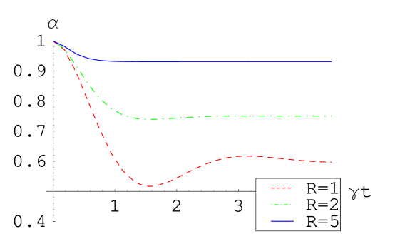
Figure 1: Fidelity of the single-qubit code with continuous bit-flip errors and correction, as a function of dimensionless time $\gamma t$, for three different values of the ratio $R=\kappa/\gamma$.

A remarkable difference, however, is that the asymptotic weight outside the code space ($1-\alpha_{*}^{NM}$) decreases with $\kappa$ as $1/\kappa^{2}$, whereas in the Markovian case the same quantity decreases as $1/\kappa$. The asymptotic value can be obtained as an equilibrium point at which the infinitesimal weight flowing out of the code space during a time step $dt$ is equal to the weight flowing into it. The latter corresponds to vanishing right-hand sides in equations (39) and (74). In Sec. V.3 we will see that the difference in that quantity for the two different types of decoherence arises from the difference in the corresponding evolutions during initial times.

V.2.3 The three-qubit bit-flip code

We will consider a model where each qubit independently undergoes the same kind of non-Markovian decoherence as the one we studied for the single-qubit code. Here the system we look at consists of six qubits—three for the codeword and three for the environment. We assume that all system qubits are coupled to their corresponding environment qubits with the same coupling strength, i.e., the Hamiltonian is

$$H=\gamma\overset{3}{\underset{i=1}{\sum}}X^{S}_{i}\otimes X^{B}_{i},$$ (77)

where the operators $X^{S}$ act on the system qubits and $X^{B}$ act on the corresponding bath qubits which are initially in the maximally mixed state. The subscripts label on which particular qubit they act. Obviously, the types of effective single-qubit errors on the density matrix of the system that can result from this Hamiltonian at any time, CP or not, will have operator elements which are linear combinations of the identity and $X^{S}$. According to the error-correction conditions for non-CP maps obtained in Ref. Shabani:07081953 , these errors are correctable by the code. Considering the form of the Hamiltonian (77) and the error-correcting map, one can see that the density matrix of the entire system at any moment is a linear combination of terms of the type

$$\varrho_{lmn,pqr}\equiv X_{1}^{l}X_{2}^{m}X_{3}^{n}\rho(0)X_{1}^{p}X_{2}^{q}X_{3}^{r}\otimes\frac{X_{1}^{l+p}}{2}\otimes\frac{X_{2}^{m+q}}{2}\otimes\frac{X_{3}^{n+r}}{2}.$$ (78)

Here the first term in the tensor product refers to the Hilbert space of the system, and the following three refer to the Hilbert spaces of the bath qubits that couple to the first, the second and the third qubits from the code respectively. The power indices $l,m,n,p,q,r$ take values $0$ and $1$ in all possible combinations, and $X^{1}=X$, $X^{0}=X^{2}=I$. (Note that $\varrho_{lmn,pqr}$ should not be mistaken with the components of the density matrix in the computational basis.) More precisely, we can write the density matrix in the form

$$\rho(t) = \underset{l,m,n,p,q,r}{\sum}(-i)^{l+m+n}(i)^{p+q+r}C_{lmn,pqr}(t)\times\varrho_{lmn,pqr},$$ (79)

where the coefficients $C_{lmn,pqr}(t)$ are real. The coefficient $C_{000,000}$ is less than or equal to the codeword fidelity (with equality when $\rho(0)=|\bar{0}\rangle\langle\bar{0}|$ or $\rho(0)=|\bar{1}\rangle\langle\bar{1}|$). Since the scheme aims at protecting an unknown codeword, we will be interested in its performance in the worst case and we will assume that the codeword fidelity is $C_{000,000}$.

The exact equations for the coefficients $C_{lmn,pqr}(t)$ and their solutions were obtained in Ref. Oreshkov:2007:022318 . Here we will present an approximation which can be obtained by perturbation theory for $\gamma\delta t\ll 1\ll\kappa\delta t$ Oreshkov:2007:022318 . The approximate system of equation reads

$$\frac{dC_{000,000}}{dt}=\frac{24}{R^{2}}\gamma C_{111,000},$$

$$\frac{dC_{111,000}}{dt}=-\frac{12}{R^{2}}\gamma(2C_{000,000}-1).$$ (80)

Comparing with (72), we see that the encoded qubit undergoes approximately the same type of evolution as that of a single qubit without error correction, but the coupling constant is effectively decreased $R^{2}/12$ times. The solution of (80) yields for the codeword fidelity

$$C_{000,000}(t)=\frac{1+\cos(\frac{24}{R^{2}}\gamma t)}{2}.$$ (81)

This solution is valid only with precision $\mathcal{O}(\frac{1}{R})$ for times $\gamma t\ll R^{3}$. If one carries out the perturbation to fourth order in $\gamma$, one obtains the approximate equations

$$\frac{dC_{000,000}}{dt}=\frac{24}{R^{2}}\gamma C_{111,000}-\frac{72}{R^{3}}\gamma(2C_{000,000}-1),$$

$$\frac{dC_{111,000}}{dt}=-\frac{12}{R^{2}}\gamma(2C_{000,000}-1)-\frac{144}{R^{3}}\gamma C_{111,000},$$ (82)

which yield for the fidelity

$$C_{000,000}(t)=\frac{1+e^{-\frac{144}{R^{3}}\gamma t}\cos(\frac{24}{R^{2}}\gamma t)}{2}.$$ (83)

We see that in addition to the effective error process which is of the same type as that of a single qubit, there is an extra Markovian bit-flip process with rate $\frac{72}{R^{3}}\gamma$. This Markovian behavior is due to the Markovian character of our error-correcting procedure which, at this level of approximation, is responsible for the direct transfer of weight between $\varrho_{000,000}$ and $\varrho_{111,111}$, and between $\varrho_{111,000}$ and $\varrho_{000,111}$. The exponential factor explicitly reveals the range of applicability of solution (81)—with precision $\mathcal{O}(\frac{1}{R})$, it is valid only for times $\gamma t$ of up to order $R^{2}$. For times of the order of $R^{3}$, the decay becomes significant and cannot be neglected. The exponential factor may also play an important role for short times of up to order $R$, where its contribution is bigger than that of the cosine. But in the latter regime the difference between the cosine and the exponent is of order $\mathcal{O}(\frac{1}{R^{2}})$, which is negligible for the precision that we consider.

Fig. 2 presents the exact solution for the codeword fidelity $C_{000,000}(t)$ as a function of the dimensionless parameter $\gamma t$ for $R=100$. For very short times after the beginning ($\gamma t\sim 0.1$), one can see a fast but small in magnitude decay (Fig.3). The maximum magnitude of this quickly decaying term obviously decreases with $R$, since in the limit of $R\rightarrow\infty$ the fidelity should remain constantly equal to $1$.

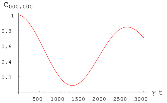
Figure 2: Long-time behavior of three-qubit system with bit-flip noise and continuous error correction. The ratio of correction rate to decoherence rate is $R=\kappa/\gamma=100$.

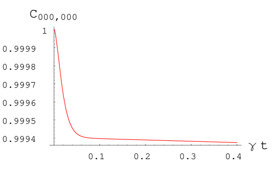
Figure 3: Short-time behavior of three-qubit system with bit-flip noise and continuous error correction. The ratio of correction rate to decoherence rate is $R=\kappa/\gamma=100$.

We see that in the limit $R\rightarrow\infty$, the evolution approaches an oscillation with an angular frequency $\frac{24}{R^{2}}\gamma$. This is the same type of evolution as that of a single qubit interacting with its environment, but the coupling constant is effectively reduced $R^{2}/12$ times. While the coupling constant can serve to characterize the decoherence process in this particular case, such a description is not valid in general. As a general measure of the effect of noise one can use the instantaneous rate of decrease of the codeword fidelity $F_{cw}$ (in our case $F_{cw}=C_{000,000}$):

$$\Lambda(F_{cw}(t))=-\frac{dF_{cw}(t)}{dt}.$$ (84)

This quantity does not coincide with the decoherence rate in the Markovian case (which can be defined naturally from the Lindblad equation), but it is a good estimate of the rate of loss of fidelity and can be used for any decoherence model. We will refer to it simply as an error rate. Since the goal of error correction is to preserve the codeword fidelity, the quantity (84) is a useful indicator of the performance of a given scheme. Note that $\Lambda(F_{cw})$ is a function of the codeword fidelity and therefore it makes sense to use it for a comparison between different cases only for identical values of $F_{cw}$. For our example, the fact that the coupling constant is effectively reduced approximately $R^{2}/12$ times implies that the error rate for a given value of $F_{cw}$ is also reduced $R^{2}/12$ times. Similarly, the reduction of $\lambda$ by the factor $r/6$ in the Markovian case implies a reduction of $\Lambda$ by the same factor. We see that the effective reduction of the error rate increases quadratically as $\kappa^{2}$ in the non-Markovian case, whereas it increases only linearly as $\kappa$ in the Markovian case.

V.3 The role of the Zeno regime

The effective continuous evolution (80) is derived under the assumption $\gamma\delta t\ll 1\ll\kappa\delta t$. The first inequality implies that $\delta t$ can be considered within the Zeno time scale of the system’s evolution without error correction. On the other hand, from the relation between $\kappa$ and $\tau_{c}$ in (9) we see that $\tau_{c}\ll\delta t$. Therefore, the time for implementing a weak error-correcting operation has to be sufficiently small so that on the Zeno time scale the error-correction procedure can be described approximately as a continuous Markovian process. This suggests a way of understanding the quadratic enhancement in the non-Markovian case based on the properties of the Zeno regime.

Let us consider again the single-qubit code from Sec. V.2.2, but this time let the error model be any Hamiltonian-driven process. We assume that the qubit is initially in the state $|0\rangle\langle 0|$, i.e., the state of the system including the bath has the form $\rho(0)=|0\rangle\langle 0|\otimes\rho_{B}(0)$. For times smaller than the Zeno time $\delta t_{Z}$, the evolution of the fidelity without error correction can be described by (67). Equation (67) naturally defines the Zeno regime in terms of $\alpha$ itself:

$$\alpha\geq\alpha_{Z}\equiv 1-C\delta t_{Z}^{2}.$$ (85)

For a single time step $\Delta t\ll\delta t_{Z}$, the change in the fidelity is

$$\alpha\rightarrow\alpha-2\sqrt{C}\sqrt{1-\alpha}\Delta t+\mathcal{O}(\Delta t^{2}).$$ (86)

On the other hand, the effect of error correction during time $\Delta t$ is

$$\alpha\rightarrow\alpha+\kappa(1-\alpha)\Delta t+\mathcal{O}(\Delta t^{2}),$$ (87)

i.e., it tends to oppose the effect of decoherence. If both processes happen simultaneously, the effect of decoherence will still be of the form (86), but the coefficient $C$ may vary with time. This is because the presence of error-correction opposes the decrease of the fidelity, and consequently can lead to an increase in the time for which the fidelity remains within the Zeno range. If this time is sufficiently long, the state of the environment could change significantly under the action of the Hamiltonian, thus giving rise to a different value for $C$ in (86) according to (68). Note that the strength of the Hamiltonian puts a limit on $C$, and therefore this constant can vary only within a certain range. The equilibrium fidelity $\alpha_{*}^{NM}$ that we obtained for the error model in Sec. V.2.2 can be thought of as the point at which the effects of error and error correction cancel out. For a general model, where the coefficient $C$ may vary with time, this leads to a quasi-stationary equilibrium. From (86) and (87), one obtains the equilibrium fidelity

$$\alpha_{*}^{NM}\approx 1-\frac{4C}{\kappa^{2}}.$$ (88)

In agreement to the result in Sec. V.2.2, the equilibrium fidelity differs from $1$ by a quantity proportional to $1/\kappa^{2}$. If one assumes a Markovian error model, for short times the fidelity changes linearly with time which leads to $1-\alpha_{*}^{M}\propto 1/\kappa$. Thus the difference can be attributed to the existence of a Zeno regime in the non-Markovian case.

This argument readily generalizes to the case of non-trivial codes if we look at the picture in the encoded basis. There each syndrome qubit undergoes a Zeno-type evolution and so do the abstract qubits associated with each error syndrome. Then using only the properties of the Zeno behavior as we did above, we can conclude that the weight outside the code space will be kept at a quasi-stationary value of order $1/\kappa^{2}$. As we argued in Sec. II, this in turn would lead to an effective decrease of the uncorrectable error rate at least by a factor proportional to $1/\kappa^{2}$.

Finally, let us make a remark about the resources needed to achieve the effect of quadratic reduction of the error rate. As it was pointed out, there are two conditions involved—one concerns the magnitude of the error-correction rate, the other concerns the time resolution of the weak error-correcting operations. Both of these quantities should be sufficiently large. There is, however, an interplay between the two, which involves the strength of the interaction required to implement the weak error correcting map (8). Let us imagine that the weak map is implemented by making the system interact weakly with an ancilla in a given state, after which the ancilla is discarded. The error correction procedure consists of a sequence of such interactions and can be thought of as a cooling process. If the time for which a single ancilla interacts with the system is $\tau_{c}$, one can verify that the parameter $\varepsilon$ in (8) would be proportional to $g^{2}\tau_{c}^{2}$, where $g$ is the coupling strength between the system and the ancilla. From (9) we then obtain that

$$\kappa\propto g^{2}\tau_{c}.$$ (89)

The two parameters that can be controlled are the interaction time and the interaction strength, and they determine the error-correction rate. Thus, if $g$ is kept constant, a decrease in the interaction time $\tau_{c}$ leads to a proportional decrease in $\kappa$ which may be undesirable. Therefore, in order to achieve a good working regime, one generally may need to adjust both $\tau_{c}$ and $g$. But in some situations decreasing $\tau_{c}$ alone can prove advantageous, since this may lead to a time resolution that reveals the non-Markovian character of an error model that was previously treated as Markovian. Then the quadratic enhancement of the performance as a function of $\kappa$ may compensate the decrease in $\kappa$, thus leading to a seemingly paradoxical result—better performance with a lower error-correction rate.

VI Outlook

In this chapter we saw that the subsystem principle can be useful for understanding various aspects of the workings of CTQEC and its performance under different noise models, as well as for the design of CTQEC protocols using protocols for the protection of a known state. However, further research is needed to understand how to construct optimal CTQEC protocols. In the case of the quantum-jump model, the code-space fidelity reaches a quasi-equilibrium value which can be used to estimate the performance of the scheme. It would be interesting to see whether an analogue of the equilibrium fidelity exists for schemes with indirect feedback. This could prove useful since stochastic evolutions are generally too complicated for analytical treatment. The equilibrium code-space fidelity can be useful also in assessing the performance of CTQEC under non-Markovian decoherence, where the description of the evolution of a system subject to CTQEC can be difficult due to the large number of environment degrees of freedom.

We discussed two main methods for obtaining CTQEC protocols from protocols for the protection of a single qubit: one based on the application of single-qubit protocols to the separate syndrome qubits, and another based on the application of single-qubit protocols to qubit subspaces associated with the different syndromes. An interesting question is whether the performance of CTQEC protocols obtained by these methods can be related to the performance of the underlying single-qubit protocols. A difficulty in the case of indirect feedback is that the noise in the encoded basis is correlated, and the effective noise on a given qubit can depend on the outcomes of the measurements on the rest of the qubits.

Another interesting direction for future investigation is to explore CTQEC for specific physical models and limitations of the control parameters (for a recent work, see Ref. Kerckhoff:0812:1246 ). We saw that applying single-qubit schemes to the syndrome qubits in the encoded basis generally requires multi-qubit operations in the original basis, but numerical simulations show that single-qubit feedback Hamiltonians in the original basis are also efficient. It would be interesting to see whether it is possible to construct efficient CTQEC protocols for non-trivial codes assuming only one- and two-qubit Hamiltonians. The ability to apply CTQEC with Hamiltonians of limited locality would be important for the scalability of this approach.

So far, CTQEC has been considered only as a method of protecting quantum memory. A natural next step is to combine this approach with universal quantum computation. An important question in this respect is whether CTQEC can be made fault tolerant. In the theory of quantum fault tolerance, logical operations and error correction are implemented mainly in terms of transversal operations between physical qubits from different blocks, where the basic operations are assumed to be discrete. Is something similar possible for CTQEC? One way of approaching this problem could be to look for fault-tolerant implementations of a universal set of weak operations using only weak transversal unitary operations and projective ancilla measurements.

Undoubtedly, the area of CTQEC offers a variety of interesting problems for future investigation. As quantum operations with limited strength or limited rate are likely to be the tools available in many quantum computing architectures in the near term, developing further the approach to protecting quantum information from noise via continuous-time feedback seems a promising direction for research.

- [1] A. Barenco, A. Berthiaume, D. Deutsch, A. Eckert, R. Jozsa and C. Macchiavello. Stabilization of quantum computations by symmetrization. SIAM Journal on Computing, 26:1541, 1997.
- [2] A. J. Leggett. Comment on “How the result of a measurement of a component of the spin of a spin-(1/2 particle can turn out to be 100”. Phys. Rev. Lett., 62:2325, 1989.
- [3] A. Peres. Quantum measurements with postselection. Phys. Rev. Lett., 62:2326, 1989.
- [4] A. Shabani and D. A. Lidar. Linear quantum error correction. e-print arXiv:0708.1953.
- [5] B. A. Chase, A. J. Landahl, and J. M. Geremia. Efficient feedback controllers for continuous-time quantum error correction. Phys. Rev. A., 77:032304, 2008.
- [6] B. Mishra and E.C.G Sudarshan. The Zeno’s paradox in quantum theory. J. Math. Phys., 18:756, 1997.
- [7] C. Ahn, A. C. Doherty, and A. J. Landahl. Continuous quantum error correction via quantum feedback control. Phys. Rev. A., 65:042301, 2002.
- [8] C. Ahn, H. W. Wiseman, and G. J. Milburn. Quantum error correction for continuously detected errors. Phys. Rev. A., 67:052310, 2003.
- [9] D. W. Kribs, R. W. Spekkens. Quantum error correcting subsystems are unitarily recoverable subsystems. Phys. Rev. A, 74:042329, 2006.
- [10] E. Knill. Protected realizations of quantum infromation. Phys. Rev. A, 74:042301, 2006.
- [11] F. Shibata and T. Arimitsu. Expansion formulas in nonequilibrium statistical mechanics. J. Phys. Soc. Jpn., 49:891, 1980.
- [12] F. Shibata, Y. Takahashi, and N. Hashitsume. A generalized stochastic liouville equation. Non-Markovian versus memoryless master equations. J. Stat. Phys., 17:171, 1977.
- [13] G. Lindblad. On the generators of quantum dynamical semigroups. Comm. Math. Phys., 48:119, 1976.
- [14] H. Krovi, O. Oreshkov, M. Ryazanov, and D. A. Lidar. Non-Markovian dynamics of a qubit coupled to an Ising spin bath. Phys. Rev. A, 76:052117, 2007.
- [15] H. M. Wiseman and J. F. Ralph. Reconsidering Rapid Qubit Purification by Feedback. New J. Phys., 8:90, 2006.
- [16] H. Nakazato, M. Namiki and S. Pascazio. Temporal behavior of quantum mechanical systems. Int. J. Mod. Phys. B, 10:247, 1996.
- [17] H.-P. Breuer and F. Petruccione. The Theory of Open Quantum Systems. Oxford University Press, Oxford, UK, 2002.
- [18] H.-P. Breuer, D. Burgarth and F. Petruccione. Non-Markovian dynamics in a spin star system: Exact solution and approximation techniques. Phys. Rev. B, 70:045323, 2004.
- [19] J. Kerckhoff, L. Bouten, A. Silberfarb, and H. Mabuchi. Physical model of continuous two-qubit parity measurement in a cavity-QED network. e-print arXiv:0812:1246.
- [20] J. P. Paz and W. H. Zurek. Continuous error correction. Proc. R. Soc. London, Ser. A, 454:355, 1998.
- [21] K. Jacobs. Optimal feedback control for the rapid preparation of a single qubit. Proc. of SPIE, 5468:355, 2004.
- [22] L. Vaidman, L. Goldenberg, and S. Wiesner. Error prevention scheme with four particles . Phys. Rev. A, 54, 1996.
- [23] M. Sarovar and G. J. Milburn. Continuous quantum error correction by cooling . Phys. Rev. A., 72:012306, 2005.
- [24] M. Sarovar, C. Ahn, K. Jacobs, and G. J. Milburn. A practical scheme for error control using feedback. Phys. Rev. A., 69:052324, 2004.
- [25] O. Oreshkov. Topics in quantum information and the theory of open quantum systems. Ph.D. thesis, University of Southern California, 2008, e-print arXiv:0812.4682.
- [26] O. Oreshkov and T. A. Brun. Weak measurements are universal. Phys. Rev. Lett., 95:110409, 2005.
- [27] O. Oreshkov and T. A. Brun. Continuous quantum error correction for non-Markovian decoherence. Phys. Rev. A, 76:022318, 2007.
- [28] O. Oreshkov, D. A. Lidar, and T. A. Brun. Operator quantum error correction for continuous dynamics. Phys. Rev. A, 78:022333, 2008.
- [29] R. Blume-Kohout, H. K. Ng, D. Poulin, and L. Viola. Constructing qubits in physical systems. Phys. Rev. Lett., 100:030501, 2008.
- [30] R. Zwanzig. Ensemble method in the theory of irreversibility. J. Chem. Phys., 33:1338, 1960.
- [31] S. Nakajima. On Quantum Theory of Transport Phenomena Steady Diffusion . Prog. Theor. Phys., 20:948, 1958.
- [32] T. A. Brun. A simple model of quantum trajectories . Am. J. Phys., 70:719, 2002.
- [33] T. Quang, M. Woldeyohannes, S. John, and G. S. Agarwal. Coherent control of spontaneous emission near a photonic band edge: a single-atom optical memory device. Phys. Rev. Lett., 79:5238, 1997.
- [34] W. H. Zurek. Reversibility and stability of information processing systems. Phys. Rev. Lett., 53:391, 1984.
- [35] Y. Aharonov and L. Vaidman. Aharonov and Vaidman reply. Phys. Rev. Lett., 62:2327, 1989.
- [36] Y. Aharonov and L. Vaidman. Properties of a quantum system during the time interval between two measurements. Phys. Rev. A, 41:11, 1990.
- [37] Y. Aharonov, D.Z. Albert, and L. Vaidman. How the result of a measurement of a component of the spin of a spin- particle can turn out to be 100. Phys. Rev. Lett., 60:1351, 1988.