Scaling Navier-Stokes Equation in Nanotubes

Abstract

On one hand, classical Monte Carlo and molecular dynamics (MD) simulations have been very useful in the study of liquids in nanotubes, enabling a wide variety of properties to be calculated in intuitive agreement with experiments. On the other hand, recent studies indicate that the theory of continuum breaks down only at the nanometer level; consequently flows through nanotubes still can be investigated with Navier-Stokes equations if we take suitable boundary conditions into account.
The aim of this paper is to study the statics and dynamics of liquids in nanotubes by using methods of non-linear continuum mechanics. We assume that the nanotube is filled with only a liquid phase; by using a second gradient theory the static profile of the liquid density in the tube is analytically obtained and compared with the profile issued from molecular dynamics simulation. Inside the tube there are two domains: a thin layer near the solid wall where the liquid density is non-uniform and a central core where the liquid density is uniform. In the dynamic case a closed form analytic solution seems to be no more possible, but by a scaling argument it is shown that, in the tube, two distinct domains connected at their frontiers still exist. The thin inhomogeneous layer near the solid wall can be interpreted in relation with the Navier length when the liquid slips on the boundary as it is expected by experiments and molecular dynamics calculations.

I Introduction

Nanofluidics is the study of the behavior of fluids that are confined to structures of nanometer characteristic dimensions (typically 1-100 nm). The possibility to observe liquids flowing at nano and micro scales, for example in carbon nanotubes Iijima ; Harris ; Tabeling , by using sophisticated experiments and complex molecular simulations using Lennard-Jones forces reveals new behaviors that are often surprising and essentially different from those usually observed at macroscopic scale Ball ; Rafii ; Bonthuis . For example, Majumder et al Majumder perform some interesting experiments and they estimate that, in nanotubes, the flow rates are four to five orders of magnitude faster than conventional fluid flow predicted through pores of 7 nm diameter and, contrary to predictions based on classical hydrodynamics, the flow rate does not decrease with increasing viscosity. Sinha et alMattia1 , in another set of experiments, indicate that in carbon nanotubes ranging from 2 to 7 nm of diameter, fluids flow with velocities up to 105 times faster than what predicted by classical fluid dynamics calculations.

The critical dimension below which confinement in nanotubes affects fluid transport is currently debated. For example if we consider water molecules between two flat, hydrophobic surfaces, it has been calculatedMattia2 that, at room temperature and atmospheric pressure, this critical dimension is around $100$ nm. Conversely, some experiments seems to show that the continuum approximation breaks down below $10$ nm in case of water, whereas experiments on capillary filling of molten metals in $0.6-1.2$ nm channels for zeolites show that the threshold for confinement effects is closer to $1$ nmMattia2 .

These incongruences may be explained by the fact that actually there is a severe computation limitation to molecular simulation, that the smooth liquid-gas interface disappears in tubes with diameter less than $8-10$ nm and therefore anomalous behavior of water may be observed in experiments with carbon nanotubes. Indeed, at this nano-size, the surface chemistry and structure of nanotubes must be controlled with a high precision to control flow rate and interaction of fluid componentsMattia2 ; Thomas . Moreover, in the framework of molecular dynamics, there are some problems to apply in a simple and direct way the propest boundary conditions necessary to generate the fluid flow. This is true especially when we consider pressure driven flowNicholls . Various methods exist to investigate fluid transport in molecular dynamics. Examples are the gravitational field method, where an artificial gravitational force – much greater than the earth’s gravitational pull – is introduced or the channel moving model, a method to trigger the flow with the viscous shear forces applied to the fluid by two moving channel walls.

Despite this indeterminacy in the literature, a relevant number of experimental studies lead to the conclusion that the classical Navier-Stokes equations are still valid at the nanoscale (see Bocquet and CharlaixBocquet and included references). The critical threshold for the applicability of continuum hydrodynamics investigated with molecular simulations and experiments may set around $1$ nm.
This value can be numerically obtained because beyond the validity of continuum equations, the value of the viscosity quantitatively remains equal to the bulk value. A typical correlation time for the stress-stress correlation function is the picosecond $\tau_{\sigma}=10^{-12}$ s, and the kinematic viscosity is $\nu=10^{-6}\text{m}^{2}\text{s}^{-1}$; consequently we obtain for water a viscous length scale $\ell_{c}=\sqrt{\nu\tau_{\sigma}}\approx 1$ nm. This observation seems to indicate, at least for water, that an unexpected nano-metric characteristic length scale naturally emerges as the lowest bound for the validity of the notion of viscosity.

The important conclusion, in analyzing the actual literature, is that for water under normal physicochemical conditions, the Navier-Stokes equation remains valid in nano-channels down to typically $1-2$ nm and the discrepancy between molecular dynamics simulations and experiments seems to be induced by the interaction of the fluid with the wall,  i.e. when we consider the boundary conditions. The evidence of this conclusion is given by the measurements and the molecular dynamics simulations of the density profile which clearly fluctuates in the vicinity of a solid wall. Therefore the main problem is not if the continuum hypothesis has to be abandoned, but whence the correct boundary conditions comes out.

Since van der Waals at the end of the $19$-th century, the fluid inhomogeneities in liquid-vapor interfaces are represented using continuous models that allows to take account of a volume energy depending on space density derivativeDunn ; Seppecher ; widom ; Kazm ; Onuki . Nevertheless, the corresponding square-gradient functional is unable to model repulsive force contributions and misses the dominant damped oscillatory packing structure of liquid interlayers near a substrate wallChernov . Furthermore, the decay lengths are correct only close to the liquid-vapor critical point where the damped oscillatory structure is subdominantEvans . In mean field theory, weighted density-functional has been used to explicitly demonstrate the dominance of this structural contribution in van der Waals thin films and to take account of long-wavelength capillary-wave fluctuations as in papers that renormalize the square-gradient functional to include capillary wave fluctuationsFischer . In contrast, fluctuations strongly damp out oscillatory structure and it is mainly for this reason that van der Waals original prediction of a hyperbolic tangent profile is so close to simulations and experimentsOno ; Rowlinson . It is possible to adjust, in phenomenological way, this state of affairs by considering the approach by Cahn in his celebrated paper studying wetting near a critical point Cahn0 . An approach that may be justified via a suitable asymptotic expression considering approximation of hard sphere molecules and London potentials for liquid-liquid and solid-liquid interactionsGouin 2 : in this way, we took account of the power-law behavior which is dominant in a thin liquid film in contact with a solid.

It is found that a similar situation may be also considered for the flow of the fluids and not only for their densities. The amended boundary conditions at a solid surface in the nano-scale framework must introduce a new length, the so-called Navier length or slip lengthBlake ; Landau ; Navier : a length relating the tangential velocity to the shear rate at the wall. Liquid slip is essential in nano-fluidic systems, as shrinking channel size leads to a dramatic increase of flow resistance and thus high-energy consumption for driving nonslip flowMH ; Ma .

The aim of the note is to justify the boundary conditions equations of nano-fluid mechanics using a simple mesoscopic approach. Our basic idea has been suggested by some experimental work regarding the measurement of the density of water in narrow pores Ball ; Bear . In such experiments it is shown that at the nanoscale the liquid must be compressible and inhomogeneous in a very narrow layer near the solid wall. In our opinion this layer is connected with the Navier length.

To support this idea we consider a nanotube made up of a cylindrical hollow tube whose diameter is of some nanometers. The nanotube is immersed in a liquid filling the interior of the nanotube, and to take account of the compressibility of the liquid, we use a second gradient theory in which the fluid is modeled by a van der Waals fluid for which the surdeformations are taken into accountvan der Waals ; Korteweg ; Cahn ; Isola . Therefore, we use a continuum theory in which the volume energy of the liquid is a function not only of the density but also of the gradient of density. The associated mathematical model may be obtained via a molecular mean field theory Gouin 1 ; Gouin 3 or via the axiomatic theory of the thermomechanics of continua Forest or by considering maximization of the entropy productionRaja1 ; Raja2 . In the following, the ideas of the van der Waals square gradient functional is used together with a condition at the wall taking account of the fluid density at its immediate proximity Gouin 2 ; Gouin 3 . By using this continuum approach, we provide a bridge between classical models of fluid mechanics and molecular simulations. A framework to develop simple analytical results in closed form of technical importance.

The plan of the paper is the following. Section 2 is devoted to the basic equations of capillary fluids using a second gradient theory. In Section 3 we consider the static problem to obtain the density profile of the liquid in the nanotube and its comparison with molecular dynamics simulation. In Section 4 we consider a dimensional analysis of Navier-Stokes equations in cylindrical coordinates and we show that the inhomogeneous character of the governing equations introduce in a natural way the Navier length. The last section is devoted to remarks and conclusion.

II Capillary fluids

II.1 Basic equations

Let us consider a fluid in a nanotube. In the immediate vicinity of the solid wall of the nanotube, the intermolecular forces are dominant and the density profile of the confined fluid is inhomogeneous; in the case of a small variation of density, the intermolecular forces induce a sharp variation of the gradient of density at the wall. In this framework the specific fluid internal energy $\varepsilon$, which is usually a function only of the density $\rho$ and the specific entropy $s$, must also take account of the gradient of density $\mathop{\rm grad}\rho$.

The second gradient model Germain is a theory of continua based on constitutive equations depending on the gradient of the density. In this case, restricting first our attention to statics, we start from a specific internal energy density in the form

$$\varepsilon=f(\rho,s,\beta)\quad\mathrm{{with}\quad}\beta=(\mathop{\rm grad}\rho)^{2},$$

and in such a way the stress tensor is Gouin 1

$$\mathbf{\mathbf{\sigma}}=-p\,\mbox{\boldmath{$I$}}-\lambda\,(\mathop{\rm grad}\rho)\otimes(\mathop{\rm grad}\rho)\equiv-p\,\mbox{\boldmath{$I$}}-\lambda\,(\mathop{\rm grad}\rho)(\mathop{\rm grad}\rho)^{T}\$$ (1)

where $\lambda\equiv 2\,\rho\,\varepsilon_{\beta}^{\prime}\ ,\ p\equiv\rho^{2}\varepsilon_{\rho}^{\prime}-\rho\,\mathop{\rm div}(\lambda\,\mathop{\rm grad}\rho)$ is the spherical part of the stress tensor, $I$ is the identity tensor and $\,{}^{T}$ denotes the transposition.
The scalar $\lambda$ - call the surdeformation coefficient of the fluid - accounts for surdeformation effects and generally depends on $\rho,s$ and $\beta$. By using kinetic theory, Rowlinson and Widom Rowlinson obtained an analogous result but with $\lambda$ constant at a given temperature $T$ and the specific energy $\varepsilon$ reads

$$\rho\,\varepsilon(\rho,s,\beta)=\rho\,\alpha(\rho,s)+\frac{\lambda}{2}\,\beta,$$

where $\alpha(\rho,s)$ is the the specific internal energy of the classical compressible fluid of pressure $P\equiv\rho^{2}\alpha_{\rho}^{\prime}$ and temperature $T\equiv\alpha_{s}^{\prime}$. Consequently, in Eq. (1),

$$p=P-\lambda\left(\frac{\beta}{2}+\rho\,\Delta\rho\right)\quad{\rm and},$$

$$\mathbf{\mathbf{\sigma}}=-P\,\mbox{\boldmath{$I$}}+\lambda\,\left(\,\frac{1}{2}\ \left((\mathop{\rm grad}\rho)^{2}+\rho\,\Delta\rho\right)\,\mbox{\boldmath{$I$}}-(\mathop{\rm grad}\rho)(\mathop{\rm grad}\rho)^{T}\right),$$

where $\Delta$ denotes the Laplacian operator. Because a convex equation of state is not able to connect the different bulks associated with a fluid interface, many authors use the van der Waals equation of state or other similar laws for the thermodynamical pressure $P$. In fact, we only consider the liquid bulk and the thermodynamical pressure $P$ is expanded near the bulk density. The equation of motion is

$$\rho\,\mathbf{a}=\mathop{\rm div}\mathbf{\mathbf{\sigma}}-\rho\mathop{\rm grad}\Omega,$$ (2)

where $\Omega$ is the extraneous force potential. Let us denote $\omega=\Omega-\lambda\,\Delta\rho$, then the equation of motion yields Gouin 1

$$\rho\,\mathbf{a}+\mathop{\rm grad}P+\rho\mathop{\rm grad}\omega=0.$$

This relation is similar to the one of the perfect fluid case but the term $\omega$ involves all capillarity effects. By neglecting the extraneous force potential, we obtain

$$\rho\,\mathbf{\mathbf{a}}+\mathop{\rm grad}P-\lambda\,\rho\,\mathop{\rm grad}\Delta\rho=0.$$ (3)

The equation of motion (3) can also be written in the form Gouin 4

$$\mathbf{a}=T\mathop{\rm grad}s-\mathop{\rm grad}H,$$

and if $T$ is constant,

$$\mathbf{a}+\mathop{\rm grad}\pi=0\,,$$ (4)

with the potentials

$$H=\varepsilon+\frac{p}{\rho}\equiv h-\lambda\,\Delta\rho\quad{\rm and}\quad\pi=H-T\,s\equiv\mu-\lambda\,\Delta\rho$$

being the generalized enthalpy and generalized chemical potential of the capillary fluid, respectively, where

$$h=\alpha+\frac{P}{\rho}\quad{\rm and}\quad\mu=\alpha+\frac{P}{\rho}-T\,s$$

are the enthalpy and the chemical potential of the classical compressible fluid, respectively Gouin 4 .

In the case of viscous fluids, the equation of motion takes account of the viscous stress tensor which is classically given by

$$\mbox{\boldmath{$\mathbf{\sigma}$}}_{v}=\eta(\mathtt{tr}\,\mbox{\boldmath{$D$}})\mbox{\boldmath{$I$}}+2\,\kappa\,\mbox{\boldmath{$D$}},$$

where $\eta$ and $\kappa$ are the shear and bulk viscosity coefficients respectively assumed to be constant and $D$ is the deformation tensor, symmetric gradient of the velocity field Sli . It would be coherent to add terms accounting for the influence of higher order derivatives of the velocity field but the over-deformation only comes from the density. In fact, as discussed in introduction, the Navier-Stokes equations correctly take account of the viscous behavior without higher order derivatives of the velocity field. Equation (2) is modified as $\rho\,\mathbf{a}=\mathop{\rm div}(\mathbf{\mathbf{\sigma}}+\mathbf{\mathbf{\sigma}}_{v})$ and for viscous liquids, Eq. (3) writes

$$\rho\,\mathbf{a}+\mathop{\rm grad}P-\lambda\,\rho\mathop{\rm grad}\,\Delta\rho-\mathop{\rm div}\mathbf{\mathbf{\sigma}}_{v}=0.$$ (5)

II.2 Boundary conditions

The forces acting between liquid and solid range over a few nanometers but can be simply described by a special surface energy. For a solid wall, the total surface energy $\varphi$ at the wall is expressed as De Gennes2 :

$$\varphi(\rho_{{}_{S}})=-\gamma_{1}\rho_{{}_{S}}+\frac{1}{2}\,\gamma_{2}\,\rho_{{}_{S}}^{2}.$$ (6)

Here $\rho_{{}_{S}}$ denotes the limit value of the liquid density at the solid wall; the constants $\gamma_{1}$, $\gamma_{2}$ and $\lambda$ are positive and can be obtained by the mean field approximation in molecular theory Gouin 2 . The boundary condition for the liquid density at the solid wall $(S)$ is associated with the free surface energy (6) and was calculated in Gouin 3

$$\lambda\left(\frac{d\rho}{dn}\right)_{|_{S}}+\varphi^{\prime}(\rho_{{}_{S}})\ =0,$$ (7)

where $\displaystyle\frac{d}{dn}\$ means the derivative following the direction of the external normal n  to the fluid. This condition corresponds to an embedding effect for the density of the fluid which is not taken into account in classical hydrodynamics.

The aim of the present note is to show that the boundary condition (7) introduce a nano-boundary layer in the tube. The byproduct of this layer is the presence of a slip velocity that we read at the micro scale and this also when we consider the classical no-slip boundary condition for the velocity field at the wall.

II.3 The chemical potential in the liquid phase

Due to the fact $\mu$ is defined to an additive constant, we denote by $\mu_{{}_{0}}(\rho)$ the chemical potential of the fluid for the liquid-vapor plane interface, such that

$$\mu_{{}_{0}}(\rho_{l})=0,$$

where $\rho_{l}$ is the liquid density in the liquid bulk corresponding to the plane liquid-vapor interface at a given temperature $T$.
To the liquid bulk of density $\rho_{l_{b}}\neq\rho_{l}$ - the density $\rho_{l_{b}}$ does not correspond to a plane liquid-vapor interface but to a mother liquid bulk associated with a droplet or a bubble and does not verify the Maxwell rule of equal area corresponding to plane liquid-vapor interfaces Derjaguin - we associate $\mu_{l_{b}}(\rho)\equiv\mu_{{}_{0}}(\rho)-\mu_{{}_{0}}(\rho_{l_{b}})$ corresponding to the chemical potential for the mother liquid bulk $\rho_{l_{b}}$. The thermodynamical potentials $\mu_{l_{b}}$ can be expended at the first order near the liquid bulk of density $\rho_{l_{b}}$

$$\mu_{l_{b}}(\rho)=\frac{c_{l}^{2}}{\rho_{l}}\left(\rho-\rho_{l_{b}}\right),$$

where $c_{l}$ is the isothermal sound velocity in the liquid bulk of density $\rho_{l}$ Gouin 7 . Similarly, the thermodynamical pressure is expended as

$$P=P_{l}+c_{l}^{2}\left(\rho-\rho_{l}\right),$$ (8)

where $P_{l}$ is the thermodynamical pressure in the liquid bulk of density $\rho_{l}$.

III Liquid density in a nanotube at equilibrium

A nanotube is represented by a hollow cylinder of length size $L$ and of small diameter $d=2R$, ($d/L\ll 1$). In Subsection IIIA, $d$ ranges from 2 to 100 nanometers and $L$ is of the order of some microns.

III.1 Profile of density by using the continuum approach

We consider solid walls with a large thickness with regards to molecular dimensions such that the surface energy verifies an expression in form (6). At equilibrium ($\mathbf{a}=0$), far from the nanotube tips and by neglecting the external forces ($\pi=\mu_{{}_{0}}-\lambda\,\Delta\rho$), Eq. (4) implies the profile of density as solution of the differential equation :

$$\lambda\,\Delta\rho=\mu_{{}_{0}}(\rho)-c,$$

where $c=\mu_{{}_{0}}(\rho_{l_{b}})$ is an additional constant associated with the density value $\rho_{l_{b}}$ in the mother bulk outside the nanotube Derjaguin . We consider the case when only the liquid fills up the nanotube. The profile of density is given by the differential equation :

$$\lambda\,\left(u_{rr}+\frac{1}{r}\,u_{r}\right)-\frac{c_{l}^{2}}{\rho_{l}}\ u=0,\qquad\mathrm{with}\quad u=\rho-\rho_{l{{}_{b}}}.$$ (9)

In cylindrical coordinates, $r$ denotes the radial coordinate. The reference length is

$$\delta_{l}=\sqrt{\frac{\lambda\,\rho{{}_{l}}}{{c_{l}}^{2}}}\,.$$

We denote by $x$ the dimensionless variable such that $r=\delta_{l}\,x$. Equation (9) reads

$$u_{xx}+\frac{1}{x}\,u_{x}-\,u=0.$$ (10)

The solutions of Eq. (10) in classical expansion form $u=\sum_{n=0}^{\infty}a_{n}x^{n}$ yield

$$\sum_{n=2}^{\infty}n^{2}\,a_{n}\,x^{n-2}-a_{n-2}\,x^{n-2}=0\quad\Longrightarrow\quad n^{2}\,a_{n}=a_{n-2}\,.$$

Due to the symmetry at $x=0$, the odd terms are null and consequently,

$$u=a_{{}_{0}}\,\sum_{p=0}^{\infty}\ \frac{1}{4^{p}\,(p\,!)^{2}}\ x^{2p}\,.$$

The series has an infinite radius of convergence. Let us define the functions

$$f(x)\equiv\sum_{p=0}^{\infty}\ \frac{1}{4^{p}\,(p\,!)^{2}}\ x^{2p}\qquad\emph{and}\qquad g(x)\equiv f^{\prime}(x)=\sum_{p=1}^{\infty}\ \frac{2p}{4^{p}\,(p\,!)^{2}}\ x^{2p-1}.$$

Consequently, $u=a_{{}_{0}}\,f(r/\delta_{l})$. The boundary condition (7) at $x=R/\delta_{l}$ yields

$$\frac{\lambda}{\delta_{l}}\,\frac{du}{dx}=\gamma_{1}-\gamma_{2}\,\rho\qquad{\rm or}\qquad a_{{}_{0}}=\frac{\delta_{l}\,\left(\gamma_{1}-\gamma_{2}\,\rho_{l_{b}}\right)}{\lambda\,g\left(\frac{R}{\delta_{l}}\right)+\gamma_{2}\,\delta_{l}\,f\left(\frac{R}{\delta_{l}}\right)}$$

and the density profile reads

$$\rho=\rho_{l_{b}}+\frac{\delta_{l}\,\left(\gamma_{1}-\gamma_{2}\,\rho_{l_{b}}\right)}{\lambda\,g\left(\frac{R}{\delta_{l}}\right)+\gamma_{2}\,\delta_{l}\,f\left(\frac{R}{\delta_{l}}\right)}\ f\left(\frac{r}{\delta_{l}}\right).$$

Densities $\rho_{l_{b}}$ and $\rho_{l}$ differ very slightly and, for the purposes of this work, can be considered as coinciding. Finally, the density profile can be written as

$$\frac{\rho}{\rho_{l}}=1+\frac{\gamma_{1}-\gamma_{2}\rho_{l}}{\delta_{l}c_{l}^{2}g\left(\frac{R}{\delta_{l}}\right)+\gamma_{2}\rho_{l}f\left(\frac{R}{\delta_{l}}\right)}f\left(\frac{r}{\delta_{l}}\right)$$ (11)

In order to visualize the density profiles (11) we consider the case of the water at $20^{\texttt{o}}$ Celsius, for which the different physical constants involved in the model are (in cgs units) as follow :
$\rho_{l}=0.998$, $c_{l}=1.478\times 10^{5}$ and $\lambda=1.17\times 10^{-5}$; the value of $\gamma_{2}$ only depends on the fluid and in the case of water $\gamma_{2}=54$ , whereas the coefficient $\gamma_{1}$ is related to the hydrophobicity or to the hydrophilicity of the solid wall Gouin 7 .

In Figure 1, different density profiles obtained for four tubes of radius $R=2,5,10$ and $100$ nanometers and for different values of $\gamma_{1}$ ($\gamma_{1}=60,75,90$), corresponding to the case when the solid wall is hydrophilic are plotted.

a)                                                              b)

c)                                                              d)

Figure 1: Density profiles for different values of $\gamma_{1}$ ($\gamma_{1}=60$, $75$, $90$) inside four nanotubes of different radius: (a) $R=2$ nm, (b) $R=5$ nm, (c) $R=10$ nm, (d) $R=100$ nm. Whatever the radius of the tube is, we note that the main part of the density variation near the wall accounts for a thickness of one nanometer and that, outside this thin layer, the liquid density is strongly constant.

The density profiles plotted in Figure 1 show that at equilibrium and independently of the diameter of the tube, the fluid domain can be separated in two cylindrical domains: the core in the center of the tube, where the density is constant, and the boundary layer near the solid wall of the tube, where the gradient of the density is significant. The thickness of the layer wherein the variation of the density takes place, is about four times the value of $\delta_{l}=0.231$ nm.

The maximal value of the density is reached on the boundary (at wall-fluid interface). It depends both on the value of the coefficient $\gamma_{1}$ and, to a lesser extent, on the diameter of the tube. The density variation inside the tube is moderate: at most $6.8\,\%$ for a strongly hydrophilic wall ($\gamma_{1}=90$) and for a tube of tiny radius $R=2$ nm.

III.2 Comparison between continuum approach and molecular dynamics simulation

Molecular dynamics (MD) simulations take account of van der Waals forces by using Lennard-Jones interaction potentials between a small number of molecules included inside the nanotube. Near the wall, MD simulations show oscillatory density profiles corresponding to the variations of the indicator function of molecular presence; moreover, the non-penetrability condition of the water molecules leads to empty domains beside the wallMattia2 ; Sony . These density fluctuations are obviously in contrast with the predictions of continuum studies corresponding to an averaging in molecular energies. In the layer beside the wall of about one nanometer, MD simulations consider a few number of molecules. As pointed out by Thomas and McGaughey Thomas2 (in Fig. 3 and Fig. 4), the graphs of density near the wall are not associated with continuous functions; the molecular distributions are gathered in cylindrical layers of about $0.2$ nm of thickness and the continuous guidelines are simply added between the density values of cylindrical layers to highlight the minima and maxima of the layer densities. Consequently, the comparison between MD simulations and the continuum approach corresponding to an averaging of the sum of molecular potentials must be done on the Gibbs adsorption of density Rowlinson at the nanotube wall involving the domain where the density differs from the bulk density. Our comparison is done by reference to the examples presented in the paper by Thomas and McGaughey. The density profile retained for comparison purpose is plotted in Figure 2.

In continuum theory of capillarity, the Young angle $\theta$ between solid-liquid surface and liquid-vapor interface is given by the relation:

$$\sigma_{{}_{SV}}-\sigma_{{}_{SL}}=\sigma_{{}_{LV}}\cos\theta,$$ (12)

where $\sigma_{{}_{SV}},\sigma_{{}_{SL}},\sigma_{{}_{LV}}$ are respectively the solid-vapor, solid-liquid and liquid-vapor superficial tensions. For water at $20^{\circ}$ Celsius and in cgs units, $\sigma_{{}_{LV}}\simeq 72$ and $\sigma_{{}_{SV}}$ can be neglected. Relation (6) expresses the value of $\sigma_{{}_{SL}}$ by mean-field theory in capillarity ($\sigma_{{}_{SL}}=\varphi(\rho_{{}_{S}})$).
Using a mean field model and London forces Gouin 2 the $\gamma_{2}$ value for water is obtained in Gouin 7 and reads $\gamma_{2}\simeq 54$. Consequently, from Eqs. (6) and (12), $\gamma_{1}\simeq 96$ and $\gamma_{1}\simeq 75$ correspond to a Young angle of $0$ degree and $45$ degree, respectively. Mattia and Gogotsi give a range of values of the Young angle for graphite Mattia2 . A realistic value for carbon nanotube can be taken as $\gamma_{1}\simeq 90$.
As a relevant example for nanotubes, the graphs of density associated with the MD simulations and continuum model are presented on Fig. 2. The MD simulation profile is rebuilt from Fig. 3 in Thomas2 , where guidelines added between minima and maxima of densities are replaced by a step function corresponding to the cylindrical layers shown in Fig. 4 in Thomas2 . Both profiles of density, corresponding to the two models, differ from the uniform bulk density value only in the nanometer range near the wall. In this domain, we calculate the total mass for the MD simulation as well as for the continuum model; consequently, we are able, in the two cases, to compare the Gibbs adsorption at the wall. To take account of the gap of density near the wall appearing in MD simulations, the cylindrical layer near the wall associated with MD simulation is considered in size 10 per cent smaller than the other layers. For carbon nanotube with radius of 10.4 nm, MD simulation predicts a Gibbs adsorption per unit length at the wall of $11.4\times 10^{-15}$ g cm^-1 whereas the continuum model predicts a Gibbs adsorption per unit length at the wall of $9.7\times 10^{-15}$ g cm^-1. These two values are of the same order. Considering that the water molecule mass is about $3\times 10^{-23}$ g, we obtain a Gibbs adsorption of about 30 molecules per nanometer length of the nanotube.

Figure 2: Density profiles inside a nanotube of radius 10.4 nm issued from molecular dynamics simulation (continuous line) and from the continuum model (dashed line). The dotted line which extends the density profile issued from MD simulation is associated with the gap of density du to the lack of water molecules beside the wall.

In Table 1 are shown the values of the Gibbs adsorption at the wall predicted by the continuum model for different values of the parameter $\gamma_{1}$. We observe that complete similarity between the two models is obtained for the perfect wetting.

$\gamma_{1}$	75	90	96
Gibbs adsorption (g cm-1)	$5.69\times 10^{-15}$	$9.74\times 10^{-15}$	$11.36\times 10^{-15}$

Table 1: Gibbs adsorption at the wall predicted by the continuum model for different values of the parameter $\gamma_{1}$

We can conclude:
In the two models we obtain the same thickness of the domain where the density of water is different from the bulk density.
The Gibbs adsorption at the wall is similar for the two models.
In the comparison, the continuous mean-field theory uses London potential which is an approximation of Lennard-Jones potential but the difference of Gibbs adsorption between the two models is, in this example, less important than the disparity between the MD simulation results obtained in different papers in the literature Majumder ; Nicholls ; Rafii ; Sony .

IV Motion of liquid in a nanotube

Due to the cylindrical symmetry of the problem, it is supposed that the velocity field $\bm{v}$ and the density $\rho$ have a radial symmetry

$$\bm{v}=u(r,z)\bm{e}_{r}+w(r,z)\bm{e}_{z},\qquad\rho=\rho(r,z),$$

where $(\bm{e}_{r},\bm{e}_{\theta},\bm{e}_{z})$ is the basis of the cylindrical coordinates $(r,\theta,z)$. The continuity equation is then written as

$$\frac{1}{r}(r\rho u)_{r}+(\rho w)_{z}=0.$$ (13)

In the following, and only for the sake of algebraic simplicity, Stokes’ hypothesis concerning the viscosity is assumed : $3\,\eta+2\,\kappa=0$. This assumption is not essential, but the analytic development is simplified and the comprehension of calculations is easier.
In the steady case $({\partial\bm{v}}/{\partial t}=0)$, the non-vanishing equations of motion (5) are written as

$$\rho\left(uu_{r}+wu_{z}\right) = -P_{r}+\kappa\left\{\frac{4}{3}\,\left[\frac{1}{r}\left(ru\right)_{r}\right]_{r}+u_{zz}+\frac{1}{3}\,w_{rz}\right\}$$ (14)

$$+\lambda\rho\left[\frac{1}{r}\left(r\rho_{r}\right)_{r}+\rho_{zz}\right]_{r},$$

$$\rho\left(uw_{r}+ww_{z}\right) = -P_{z}+\kappa\left\{\frac{1}{r}\left(rw_{r}\right)_{r}+\frac{4}{3}\,w_{zz}+\frac{1}{3}\left[\frac{1}{r}\left(ru\right)_{r}\right]_{z}\right\}$$ (15)

$$+\lambda\rho\left[\frac{1}{r}\left(r\rho_{r}\right)_{r}+\rho_{zz}\right]_{z}.$$

The solution of this set of equations cannot be obtained analytically. However, an approached velocity profile can be obtained by re-scaling Eqs (13–15). The re-scaling procedure, which is the object of the present section, is made with respect to a small geometrical parameter $\epsilon=d/L$ but also with respect to a small physical quantity $\tau=\delta_{l}/d$. To this goal, the following set of dimensionless variables – indicated with  $\tilde{}$  –  is introduced :

$$r=d\tilde{r},\quad z=L\tilde{z},\quad u=\hat{w}\tilde{u},\quad w=\hat{w}\tilde{w},\quad\rho=\rho_{l}\tilde{\rho},$$

where $\hat{w}$ is a reference velocity of the liquid; we chose the mean velocity in the nanotube estimated by its corresponding value in the case of a Poiseuille flow

$$\hat{w}=-\frac{d^{2}\,\mathop{\rm grad}\Delta P}{32\,\kappa},$$ (16)

where $\mathop{\rm grad}\Delta P$ denotes the gradient of the pressure difference between the nanotube extremities. In so doing, the continuity equation becomes

$$(\tilde{r}\tilde{\rho}\tilde{u})_{\tilde{r}}+\epsilon\,\tilde{r}(\tilde{\rho}\tilde{w})_{\tilde{z}}=0.$$ (17)

If we denote by $Re=\rho_{l}\,\hat{w}\,d/\kappa$ the Reynolds number and by $M=\hat{w}/c_{l}$ the Mach number, and taking account of Eq.(8), the momentum equations become

$$Re\,\tilde{\rho}\left(\tilde{u}\tilde{u}_{\tilde{r}}+\epsilon\tilde{w}\tilde{u}_{\tilde{z}}\right) = -\frac{Re}{M^{2}}\,\tilde{\rho}_{\tilde{r}}+\frac{4}{3}\left[\frac{1}{\tilde{r}}\left(\tilde{r}\tilde{u}\right)_{\tilde{r}}\right]_{\tilde{r}}+\epsilon^{2}\tilde{u}_{\tilde{z}\tilde{z}}+\frac{1}{3}\,\epsilon\tilde{w}_{\tilde{r}\tilde{z}}$$ (18)

$$+\frac{Re}{M^{2}}\,\tau^{2}\tilde{\rho}\left[\frac{1}{\tilde{r}}\left(\tilde{r}\tilde{\rho}_{\tilde{r}}\right)_{\tilde{r}}+\epsilon^{2}\tilde{\rho}_{\tilde{z}\tilde{z}}\right]_{\tilde{r}},$$

$$Re\,\tilde{\rho}\left(\tilde{u}\tilde{w}_{\tilde{r}}+\epsilon\tilde{w}\tilde{w}_{\tilde{z}}\right) = -\frac{Re}{M^{2}}\,\epsilon\tilde{\rho}_{\tilde{z}}+\frac{1}{\tilde{r}}\left(\tilde{r}\tilde{w}_{\tilde{r}}\right)_{\tilde{r}}+\frac{4}{3}\,\epsilon^{2}\tilde{w}_{\tilde{z}\tilde{z}}+\frac{1}{3}\,\epsilon\left[\frac{1}{\tilde{r}}\left(\tilde{r}\tilde{u}\right)_{\tilde{r}}\right]_{\tilde{z}}$$ (19)

$$+\frac{Re}{M^{2}}\,\epsilon\tau^{2}\tilde{\rho}\left[\frac{1}{\tilde{r}}\left(\tilde{r}\tilde{\rho}_{\tilde{r}}\right)_{\tilde{r}}+\epsilon^{2}\tilde{\rho}_{\tilde{z}\tilde{z}}\right]_{\tilde{z}}.$$

In order to evaluate the respective size of the coefficients of Eqs. (17–19) some numerical reference values for different physical variables should be considered. These numerical values are expressed in cgs units as follows :

$$L=10^{-2},\quad c_{l}=1.478\times 10^{5},\quad\kappa=0.01,\quad\rho_{l}=0.998,\quad\delta_{l}=2.31\times 10^{-8},$$

and nanotubes of four different diameters are considered :

$$d\in\left\{4\times 10^{-7},\quad 10^{-6},\quad 2\times 10^{-6},\quad 2\times 10^{-5}\right\}.$$

We will assume $\mathop{\rm grad}\Delta P=-10^{6}$ (corresponding to one atmosphere per centimeter length of the nanotube). Consequently, the numerical values of the coefficients in equations (17–19) are resumed in Table 2.

d = 2 R	$4\times 10^{-7}$	$10^{-6}$	$2\times 10^{-6}$	$2\times 10^{-5}$
$\epsilon$	$4\times 10^{-5}$	$10^{-4}$	$2\times 10^{-4}$	$2\times 10^{-3}$
$\tau$	$5.8\times 10^{-2}$	$2.3\times 10^{-2}$	$1.16\times 10^{-2}$	$1.16\times 10^{-3}$
$\hat{w}$	$5\times 10^{-7}$	$3.13\times 10^{-6}$	$1.25\times 10^{-5}$	$1.25\times 10^{-3}$
$Re$	$2\times 10^{-11}$	$3.12\times 10^{-10}$	$2.5\times 10^{-9}$	$2.5\times 10^{-6}$
$M$	$3.38\times 10^{-12}$	$2.11\times 10^{-11}$	$8.46\times 10^{-11}$	$8.46\times 10^{-9}$
${Re}\,\epsilon/M^{2}$	$6.98\times 10^{7}$
$\xi=4\tau$	$0.23$	$0.092$	$0.046$	$0.0046$
${Re}\,\epsilon\,\xi^{2}/M^{2}$	$3.73\times 10^{6}$	$5.97\times 10^{5}$	$1.49\times 10^{5}$	$1.49\times 10^{3}$

Table 2: Numerical values of the coefficients in equations (17–19)

It is worth noting that the coefficient ${Re}\,\epsilon/M^{2}$ is independent of the diameter of the nanotube. Moreover, when $\mathop{\rm grad}\Delta P=-1$ corresponding to a very low pressure difference between the tips of the nanotube, the term ${Re}\,\epsilon/M^{2}$ is simply multiplied by $10^{-6}$ which always remains very large with respect to the other quantities.

As suggested by the density profiles at equilibrium, the analyze of the liquid flow will be separately carried in two cylindrical domains:
$\quad-$ In the core, containing the axis of the tube, where the liquid density at equilibrium is independent of $r$,
$\quad-$ In the boundary layer, near the solid wall of the tube, where the density gradient is significant. Based on the observations made in Section III, the thickness of the boundary layer is of the order of 4$\delta_{l}$.
Consequently, the equation of motion is solved in the two different regions by using a small length parameter. Using a matched asymptotic expansion, different analytic solutions are obtained in both zones. An immediate outcome should be that the inner part of the boundary layer solution matches the outer part of bulk flow.

IV.1 Liquid flow in the core

Due to $\epsilon\ll 1$, the main term of Eq. (17) yields

$$(\tilde{r}\tilde{\rho}\tilde{u})_{\tilde{r}}=0$$

and consequently,

$$\tilde{u}=\frac{\psi(\tilde{z})}{\tilde{r}\,\tilde{\rho}},$$

where $\psi$ is a function of $\tilde{z}$ only. Since $\tilde{u}$ must be bounded when $\tilde{r}$ goes to zero, we get $\psi(\tilde{z})=0$ and consequently $\tilde{u}=0$.
Considering that $u(r,z)\equiv 0$, Eq. (17) yields

$$(\tilde{\rho}\tilde{w})_{\tilde{z}}=0.$$

Then, the momentum equations become

$$0 = -\frac{Re}{M^{2}}\,\tilde{\rho}_{\tilde{r}}+\frac{1}{3}\,\epsilon\tilde{w}_{\tilde{r}\tilde{z}}+\frac{Re}{M^{2}}\,\tau^{2}\tilde{\rho}\left[\frac{1}{\tilde{r}}\left(\tilde{r}\tilde{\rho}_{\tilde{r}}\right)_{\tilde{r}}+\epsilon^{2}\tilde{\rho}_{\tilde{z}\tilde{z}}\right]_{\tilde{r}},$$ (20)

$$\epsilon Re\,\tilde{\rho}\left(\tilde{w}\tilde{w}_{\tilde{z}}\right) = -\frac{Re}{M^{2}}\,\epsilon\tilde{\rho}_{\tilde{z}}+\frac{1}{\tilde{r}}\left(\tilde{r}\tilde{w}_{\tilde{r}}\right)_{\tilde{r}}+\frac{4}{3}\,\epsilon^{2}\tilde{w}_{\tilde{z}\tilde{z}}+\frac{Re}{M^{2}}\,\epsilon\tau^{2}\tilde{\rho}\left[\frac{1}{\tilde{r}}\left(\tilde{r}\tilde{\rho}_{\tilde{r}}\right)_{\tilde{r}}+\epsilon^{2}\tilde{\rho}_{\tilde{z}\tilde{z}}\right]_{\tilde{z}}.\qquad\qquad$$ (21)

In agreement with the coefficient values of Table 2, the main parts of the momentum equations are obtained by retaining the dominant terms in Eqs. (20–21) :

$$\tilde{\rho}_{\tilde{r}}=0\qquad{\rm and}\qquad\frac{1}{\tilde{r}}\left(\tilde{r}\tilde{w}_{\tilde{r}}\right)_{\tilde{r}}=\frac{Re}{M^{2}}\,\epsilon\,\tilde{\rho}_{\tilde{z}}.$$ (22)

Note that, due to $\tilde{\rho}_{\tilde{r}}=0$, the term $\displaystyle\frac{Re}{M^{2}}\,\epsilon\tau^{2}\tilde{\rho}\frac{1}{\tilde{r}}\left(\tilde{r}\tilde{\rho}_{\tilde{r}}\right)_{\tilde{r}\tilde{z}}$, which should appear in the second equation (22) is null.

Equations (22) can be explicitly integrated and yield

$$\tilde{\rho}=\tilde{\rho}(\tilde{z})\qquad{\rm and}\qquad\tilde{w}(\tilde{r},\tilde{z})=-\frac{Re}{4\,M^{2}}\,\epsilon\tilde{\rho}^{\prime}\left(k_{0}-\tilde{r}^{2}\right)$$ (23)

where $k_{0}$ is a constant to be determined by the boundary conditions. Introducing this velocity field in the continuity equation we obtain

$$\tilde{\rho}(\tilde{z})=\sqrt{h_{0}\tilde{z}+h_{1}},$$

where the constants $h_{0}$ and $h_{1}$ must be determined from the inlet and outlet bulk densities. For example, if we assume that the inlet bulk density is $\tilde{\rho}(0)=1$, the outlet bulk density $\tilde{\rho}(1)$ derives from Eq. (8) when $\mathop{\rm grad}\Delta P=-10^{6}$ :

$$\rho(L)-\rho(0)=\frac{\Delta P}{c_{l}^{2}}\simeq-0.46\times 10^{-6}.$$

Consequently, $h_{1}=1$ and $h_{0}=-0.92\times 10^{-6}$.

IV.2 Liquid flow in the boundary layer

In the boundary layer, $\tilde{r}$ is always different from zero and the reasoning made in Section IV no longer works. From Eq. (17) we get that $\tilde{u}$ is of order of $\epsilon\tilde{w}$. Then, introducing $\bar{u}$ as

$$\tilde{u}=\epsilon\bar{u},$$

the continuity equation becomes

$$\frac{1}{\tilde{r}}(\tilde{r}\tilde{\rho}\bar{u})_{\tilde{r}}+(\tilde{\rho}\tilde{w})_{\tilde{z}}=0.$$

To have an idea of what happens near the wall of the nanotube, we have to translate and re-scale $\tilde{r}$ such that $\tilde{r}=1/2-\xi\overline{r}$. Hence, on the boundary of the nanotube where $\tilde{r}=1/2$, we get $\overline{r}=0$. The value of $\xi$ is determined by the condition $\overline{r}=1$ on the separating surface between the core and the boundary layer where $\tilde{r}=1/2-4\tau$, and we get $\xi=4\tau$. Therefore, the continuity equation is :

$$-\frac{1}{1-2\xi\overline{r}}\,[(1-2\xi\overline{r})\tilde{\rho}\bar{u}]_{\overline{r}}+\xi(\tilde{\rho}\tilde{w})_{\tilde{z}}=0,$$

and the momentum equations are :

$$Re\,\epsilon^{2}\tilde{\rho}\left(-\xi\bar{u}\bar{u}_{\overline{r}}+\xi^{2}\tilde{w}\bar{u}_{\tilde{z}}\right) = \frac{Re}{M^{2}}\,\xi\tilde{\rho}_{\overline{r}}+\frac{4}{3}\,\epsilon\left[\frac{1}{1-2\xi\overline{r}}\left((1-2\xi\overline{r})\bar{u}\right)_{\overline{r}}\right]_{\overline{r}}$$

$$+\epsilon^{3}\xi^{2}\bar{u}_{\tilde{z}\tilde{z}}-\frac{1}{3}\,\epsilon\,\xi\tilde{w}_{\overline{r}\tilde{z}}-\frac{Re}{16\,M^{2}}\,{\xi\,\tilde{\rho}}\left[\frac{1}{1-2\xi\overline{r}}\left((1-2\xi\overline{r})\tilde{\rho}_{\overline{r}}\right)_{\overline{r}}+\epsilon^{2}\xi^{2}\tilde{\rho}_{\tilde{z}\tilde{z}}\right]_{\overline{r}},$$ (24)

$$Re\,\epsilon\,\tilde{\rho}\left(-\xi\bar{u}\tilde{w}_{\overline{r}}+\xi^{2}\tilde{w}\tilde{w}_{\tilde{z}}\right) = -\frac{Re}{M^{2}}\,\epsilon\,\xi^{2}\tilde{\rho}_{\tilde{z}}+\frac{1}{1-2\xi\overline{r}}\left[(1-2\xi\overline{r})\tilde{w}_{\overline{r}}\right]_{\overline{r}}+\frac{4}{3}\,\epsilon^{2}\xi^{2}\tilde{w}_{\tilde{z}\tilde{z}}$$ (25)

$$-\frac{1}{3}\,\epsilon^{2}\xi\left[\frac{1}{1-2\xi\overline{r}}\left((1-2\xi\overline{r})\bar{u}\right)_{\overline{r}}\right]_{\tilde{z}}+\frac{Re}{16\,M^{2}}\,\epsilon\,\xi^{2}\tilde{\rho}\left[\frac{1}{1-2\xi\overline{r}}\left((1-2\xi\overline{r})\tilde{\rho}_{\overline{r}}\right)_{\overline{r}}+\epsilon^{2}\xi^{2}\tilde{\rho}_{\tilde{z}\tilde{z}}\right]_{\tilde{z}}.\qquad$$

Then, neglecting the terms whose coefficients are very small, we obtain from Eq. (24) :

$$\frac{Re}{M^{2}}\,\xi\,\tilde{\rho}_{\overline{r}}-\frac{Re}{16\,M^{2}}{\xi\,\tilde{\rho}}\left[\frac{1}{1-2\xi\overline{r}}\left((1-2\xi\overline{r})\tilde{\rho}_{\overline{r}}\right)_{\overline{r}}\right]_{\overline{r}}=0.$$

This equation can be partially integrated and gives :

$$\log(\tilde{\rho})-\frac{1}{16}\left[\frac{1}{1-2\xi\overline{r}}\left((1-2\xi\overline{r})\tilde{\rho}_{\overline{r}}\right)_{\overline{r}}\right]=k(\tilde{z})$$

where $k$ is an unknown fonction of $\tilde{z}$ only. Then :

$$\tilde{\rho}_{\tilde{z}}-\frac{1}{16}\tilde{\rho}\left[\frac{1}{1-2\xi\overline{r}}\left((1-2\xi\overline{r})\tilde{\rho}_{\overline{r}}\right)_{\overline{r}}\right]_{\tilde{z}}=\tilde{\rho}k^{\prime}(\tilde{z}).$$ (26)

Taking account of Eq. (26), the dominant terms of Eq. (25) write :

$$-\frac{Re}{M^{2}}\,\epsilon\,\xi^{2}\,\tilde{\rho}_{\tilde{z}}+\frac{Re}{16\,M^{2}}\,\epsilon\,\xi^{2}\tilde{\rho}\,\frac{1}{1-2\xi\overline{r}}\left[(1-2\xi\overline{r})\tilde{\rho}_{\overline{r}}\right]_{\overline{r}\tilde{z}}=-\frac{Re}{M^{2}}\,\epsilon\,\xi^{2}\,\tilde{\rho}k^{\prime}(\tilde{z})$$

which should be equal to zero; therefore $k(\tilde{z})$ is constant and Eq. (25) is restricted to :

$$\frac{1}{1-2\xi\overline{r}}\left((1-2\xi\overline{r})\tilde{w}_{\overline{r}}\right)_{\overline{r}}=0.$$

The solution of this equation with the no-slip boundary condition is

$$\tilde{w}=-\frac{m(\tilde{z})}{2\xi}\log(1-2\xi\overline{r})=-\frac{m(\tilde{z})}{2\xi}\log(2\tilde{r}),$$ (27)

where $m(\tilde{z})$ is a function to be determined with the continuity condition of the velocity field through the surface separating the core and the boundary layer, i.e. for $\tilde{r}=1/2-\xi$. From Eqs. (23) and (27) we get :

$$-\frac{Re}{4M^{2}}\,\epsilon\tilde{\rho}^{\prime}(\tilde{z})\,\left[k_{0}-\left(\frac{1}{2}-\xi\right)^{2}\right]=-\frac{m(\tilde{z})}{2\xi}\log(1-2\xi).$$

Therefore $m$ is proportional with $\tilde{\rho}^{\prime}$ :

$$m(\tilde{z})=\frac{\xi\,\epsilon Re}{8M^{2}}\frac{4k_{0}-(1-2\xi)^{2}}{\log(1-2\xi)}\,\tilde{\rho}^{\prime}(\tilde{z})$$ (28)

IV.3 Velocity profile in the nanotube

From Eqs. (23) (27) and (28) the expression of the velocity field $\tilde{w}(\tilde{r},\tilde{z})$ in the whole domain is :

$$\tilde{w}(\tilde{r},\tilde{z})=\left\{\begin{array}[]{l}\displaystyle-\frac{\epsilon Re}{4\,M^{2}}\,\tilde{\rho}^{\prime}(\tilde{z})\left(k_{0}-\tilde{r}^{2}\right),\qquad 0\leqslant\tilde{r}\leqslant\frac{1}{2}-\xi\\[8.5359pt] \displaystyle-\frac{\epsilon Re}{16M^{2}}\frac{4k_{0}-(1-2\xi)^{2}}{\log(1-2\xi)}\,\tilde{\rho}^{\prime}(\tilde{z})\log(2\tilde{r}),\qquad\frac{1}{2}-\xi\leqslant\tilde{r}\leqslant\frac{1}{2}\end{array}.\right.$$ (29)

It depends on the constant $k_{0}$ which is determined by the following average condition (which expresses the fact that the average of $w$ on the outlet section of the tube is equal to $\hat{w}$) :

$$\frac{4}{\pi}\int_{0}^{2\pi}\int_{0}^{1/2}\tilde{w}(\tilde{r},1)\,\tilde{r}\,\textrm{d}\tilde{r}\textrm{d}\theta=1\quad\Leftrightarrow\quad\int_{0}^{1/2}\tilde{w}(\tilde{r},1)\,\tilde{r}\,\textrm{d}\tilde{r}=\frac{1}{8}.$$

We obtain :

$$k_{0}=\left(\frac{1}{2}-\xi\right)^{2}+\frac{8+\alpha(1-2\xi)^{4}}{16\alpha(1-\xi)\xi}\log(1-2\xi),$$

where $\alpha=\displaystyle\frac{\epsilon Re}{4\,M^{2}}\,\tilde{\rho}^{\prime}(1)$ has a numerical value independent of the diameter of the nanotube, $\alpha\simeq-8.0$.

In Figure 3 are plotted the profiles of the normalized velocity $\tilde{w}$ (29) in the four nanotubes. The motions are rather slow, the maximum of the velocity being about two times $\hat{w}$ (see Table 2). As already mentioned, it is assumed that the boundary layer (in grey on the Figure), where the liquid is inhomogeneous, is the same than at equilibrium (see Section 3 and Fig. 3). Obviously, due to the condition (28) the graphs are continuous between the boundary layer and the core (see Fig. 3).

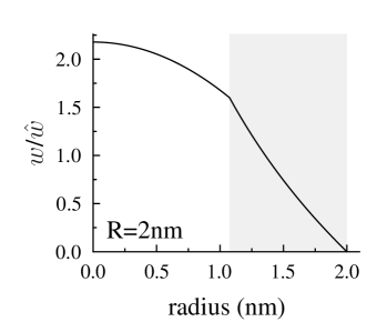
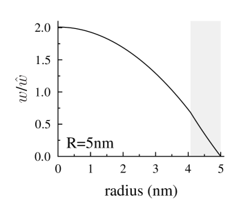
a)                                                              b)

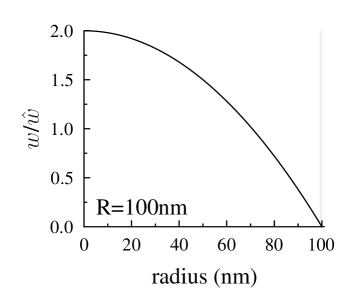
c)                                                              d)

Figure 3: Velocity profiles in nanotubes of different radius: (a) $R=2$ nm, (b) $R=5$ nm, (c) $R=10$ nm, (d) $R=100$ nm. The plots simply show the inner and outer regions up to and including a distinct point of separation of the two analytic representations. The region near the wall is represented in a grey area

As for the classical Poiseuille flow, in the core the velocities profiles are parabolic (see Eq. (23)). In Figure 4 are plotted the profiles of the normalized velocity $\tilde{w}$ near the axis of the tube, in the four nanotubes. For larger nanotubes (5 nm to 100 nm) the normalized velocity is almost the same and the influence of the boundary wall on the normalized velocity in the core is less important that in the case of a thin tube (2 nm). It is worth noting that the flow near the axis of a thin nanotube is “proportionally” faster that the flow in larger nanotubes.

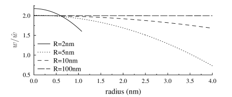
Figure 4: Velocity profiles near the axis of the tube for four different nanotubes

Since the function $\tilde{\rho}^{\prime}(\tilde{z})$ has a weak variation inside the interval $[0,1]$, the value of the velocity (29) at the interface between the core and the boundary layer can be approximated by :

$$\left.\tilde{w}\right|_{\tilde{r}=1/2-\xi}=-\frac{\tilde{\rho}^{\prime}(\tilde{z})}{\tilde{\rho}^{\prime}(1)}\frac{8+\alpha(1-2\xi)^{4}}{16(1-\xi)\xi}\log(1-2\xi)\simeq-\frac{8+\alpha(1-2\xi)^{4}}{16(1-\xi)\xi}\log(1-2\xi).$$

Whatever the radius of the nanotube, the density variation takes place in a thin layer for a thickness of one nanometer. Outside of this thin boundary layer, the liquid density is constant. In fact, due to the very thin boundary layer, we may consider the motion as the motion of an incompressible liquid in the core when $r\in[0,R-4\delta_{l}]$ and define a boundary slip velocity as the velocity obtained for $r=R-4\delta_{l}$ corresponding to the frontier of the inhomogeneous liquid layer. In this case, the Navier Length $b$ corresponds to De Gennes

$$\frac{w}{b}=\frac{\partial w}{\partial r}\qquad{\rm when}\qquad r=R-4\delta_{l}.$$ (30)

Due to $w=0$ when $r=R$, and the fact that the variations of $w$ in the boundary layer are smooth enough, the graph of velocity in the boundary layer is near a straight line. Then, for water at $20^{\texttt{o}}$ Celsius, the Navier length $b$ corresponds to the boundary layer thickness which is about one nanometer and, due to Eq. (16), the slip velocity is

$$w_{g}=w_{{}_{|r=R-4\delta_{l}}}=\tilde{w}_{{}_{|\tilde{r}=1/2-\xi}}\,\hat{w}=\frac{8+\alpha(1-2\xi)^{4}}{16(1-\xi)\xi}\log(1-2\xi)\frac{d^{2}\,\mathop{\rm grad}\Delta P}{32\,\kappa}.$$ (31)

Consequently, Eqs. (30) and (31) yield the boundary conditions for the Hagen-Poiseuille flow in the core.

The values of the slip velocity $w_{g}$ are given in Table 3 (in c.g.s. system units). The case when $R=100$ nm is close from a flat thin boundary layer and in our model, the Navier length is constant whatever the radius of the nanotube is.

d = 2 R	$4\times 10^{-7}$	$10^{-6}$	$2\times 10^{-6}$	$2\times 10^{-5}$
$w_{g}$	$8.0\times 10^{-7}$	$2.127\times 10^{-6}$	$4.424\times 10^{-6}$	$4.603\times 10^{-5}$

Table 3: Numerical values of the slip velocity $w_{g}$ following the radius value of the nanotube

V Conclusion and comments

The question about the correct set of boundary conditions at the nanoscale is recurrent in both molecular dynamics simulation and the applications of continuum fluid-mechanics. Clearly, the classical no-slip boundary condition of macroscopic fluid mechanics does not apply, and in confined nano-flows, it is necessary to get a deep understanding of the interfacial friction phenomena between fluid and wall.

Using the classical terminology we say that the slip velocity is the tangential velocity of the fluid at the solid wall determined by a surface friction coefficient $k$, while the Navier length represents the length given by the ratio $k/\eta$ (De Gennes , Fig. 1). Here we use a continuum model generalizing Navier-Stokes equation via an internal energy function of the deformation and the surdeformation of the fluid. For this reason the boundary effects predicted by the model are deeply different from what we see in classical Navier-Stokes equations. This model accounts for an embedding effect at the solid surfaces where the liquid is subjected to strong variations of density. The intermolecular forces, mainly by capillarity effects, create an inhomogeneous layer at the wall where slippage of the liquid is possible. The thickness of the layer depends on the molecular length $\delta_{l}$ and consequently on the temperature through the surdeformation coefficient $\lambda$ of the fluid and the isothermal sound speed ${c}_{l}$. The results are compatible with MD simulations: the Gibbs adsoption is of the same order and the inhomogeneous density layer has the same thickness in the two models. The thickness of the inhomogeneous layer is the Navier length; the slip velocity is the fluid velocity evaluated at the internal boundary of the inhomogeneous layer.

Finally, the simple proposed model highlights the following points:
The continuum mechanics approach is in intuitive agreement with what is expected by experiments and confirms the adequation of van der Waals’ model in nanoscale framework by using a convenient representation of the fluid-solid interaction.
The continuum mechanics approach is important to obtain simple analytical solutions for simple flow geometries.

Acknowledgements: GS is partially supported by PRIN project ’Matematica e meccanica dei sistemi biologici e dei tessuti molli’; GS & HG are also supported by ’Institut Carnot Star’ for the stays during the year 2012 and the collaboration between Aix-Marseille Université and Università degli Studi di Perugia.

References

- (1) S. Iijima, ”Helical microtubules of graphitic carbon,” Nature 354, 56 (1991).
- (2) P. J. F. Harris, Carbon Nanotubes and Related Structures, New Materials for the Twenty-First Century (Cambridge University Press, Cambridge, 1999).
- (3) P. Tabeling, Introduction to microfluidics (Oxford University Press Publication, Oxford, 2006).
- (4) R. C. Ball, and R. Evans, ”The density profile of a confined fluid,” Mol. Phys. 63, 159 (1988).
- (5) H. Rafii-Tabar, Computational Physics of Carbon Nanotubes (Cambridge University Press, Cambridge, 2009).
- (6) D. J. Bonthuis, K. F. Rinne, K. Falk, C. Nadir Kaplan, D. Horinek, A. Nihat Berker, L. Bocquet, and R. R. Netz, ”Theory and simulations of water flow through carbon nanotubes: prospects and pitfalls,” J. Phys.: Condens. Matter 23, 184110 (2011).
- (7) M. Majumder, N. Chopra, R. Andrews , and B. J. Hinds, ”Enhanced flow in carbon nanotubes,” Nature 438, 44 (2005).
- (8) S. Sinha, M. Pia Rossi, D. Mattia , Y. Gogotsi, and H. H. Bau, ”Induction and measurement of minute flow rates through nanopipes,” Phys. Fluids 19, 013603 (2007).
- (9) D. Mattia, and Y. Gogotsi, ”Review: static and dynamic behavior of liquids inside carbon nanotubes,” Microfluid. Nanofluid 5, 289 (2008).
- (10) J. A. Thomas, and A. J. H. McGaughey, ”Reassessing fast water transport through carbon nanotubes,” Nano Lett. 8, 2788 (2008).
- (11) W. D. Nicholls, M. K. Borg, and J. M. Reese, ”Molecular dynamics simulations of liquid flow in and around carbon nanotubes,” in Proceedings of ASME 2010 3rd Joint US-European Fluids Engineering Summer Meeting and 8th International Conference on Nanochannels, Microchannels, and Minichannels (FEDSM-ICNMM, Montreal, Canada, 2010) p. 1.
- (12) L. Bocquet, and E. Charlaix, ”Nanofluidics, from bulk to interfaces, a Critical Review,” Chem. Soc. Rev. 39, 1073 (2010).
- (13) J. E. Dunn, R. Fosdick and M. Slemrod (Eds.), Shock induced transitions and phase structures, The IMA Volumes in Mathematics and its Applications, vol. 52 (Springer, Berlin, 1993).
- (14) P. Seppecher, ”Moving contact lines in the Cahn-Hilliard theory,” Int. J. Eng. Sci. 34, 977 (1996).
- (15) B. Widom, ”What do we know that van der Waals did not know?,” Physica A 263, 500 (1999).
- (16) B. Kazmierczak, and K. Piechór, ”Parametric dependence of phase boundary solution to model kinetic equations,” ZAMP 53, 539 (2002).
- (17) A. Onuki, ”Dynamic van der Waals theory,” Phys. Rev. E 75, 036304 (2007).
- (18) A. A. Chernov, and L. V. Mikheev, ”Wetting of solid surfaces by a structured simple liquid: effect of fluctuations” Phys. Rev. Lett. 60, 2488 (1988).
- (19) R. Evans, ”The nature of liquid -vapour interface and other topics in the statistical mechanics of non-uniform classical fluids,” Adv. Phys. 28, 143 (1979).
- (20) M. E. Fisher, and A. J. Jin, ”Effective potentials, constraints, and critical wetting theory,” Phys. Rev. B 44, 1430 (1991).
- (21) S. Ono and S. Kondo, Molecular theory of surface tension in liquid, in: Structure of Liquids, Edited by S. Flügge, Encyclopedia of Physics, X, (Springer, Berlin, 1960).
- (22) J. S. Rowlinson and B. Widom, Molecular Theory of Capillarity (Clarendon Press, Oxford, 1984).
- (23) J. W. Cahn, ”Critical point wetting,” J. Chem. Phys. 66, 3667 (1977).
- (24) H. Gouin, ”Energy of interaction between solid surface and liquids,” J. Phys. Chem. B 102, 1212 (1998) & arXiv:0801.4481.
- (25) C. L. Navier, ”Mémoire sur les lois du mouvement des fluides,” Mémoires Acad. R. Sci. Inst. France 6, 389 (1823).
- (26) L. Landau and E. Lifchitz, Fluid Mechanics (Mir Edition, Moscow, 1958).
- (27) T. D. Blake, ”Slip between a liquid and a solid - D.M. Tolstoi (1952) theory reconsidered,” Colloids Surf. 47, 135 (1990).
- (28) M. T. Matthews, and J. M. Hill, ”On three simple experiments to determine slip lengths Microfluid. Nanofluid.,” 6, 611 (2009).
- (29) M. D. Ma, L. Shen, J. Sheridan, J. Z. Liu, C. Chen, and Q. Zheng, ”Friction of water slipping in carbon nanotubes,” Phys. Rev. E 83, 036316 (2011).
- (30) J. Bear, Dynamics of Fluids in Porous Media (Dover Publ., New York, 1988).
- (31) J. D. van der Waals, Translation by J. S. Rowlinson, ”The thermodynamic theory of capillarity under the hypothesis of a continuous variation of density,” J. Stat. Phys. 20, 197 (1979).
- (32) D. J. Korteweg, ”Sur la forme que prennent les équations du mouvement des fluides si l’on tient compte des forces capillaires,” Arch. Néerlandaises, II, VI, 1 (1901). Also presented in C. Truesdell and W. Noll, The non-linear field theories of mechanics, Third Edition, Edited by S.S. Antman, ”Korteweg’s theory of capillarity,” (Springer, Berlin, 2004) p. 513.
- (33) J. W. Cahn, and J. E. Hilliard, ”Free energy of a nonuniform system. III. Nucleation in a two-component incompressible fluid,” J. Chem. Phys. 31, 688 (1959).
- (34) F. dell’Isola, H. Gouin, and G. Rotoli, ”Nucleation of spherical shell-like interfaces by second gradient theory: numerical simulations,” Eur. J. Mech., B/Fluids, 15, 545 (1996) & arXiv:0906.1897.
- (35) H. Gouin, Utilization of the second gradient theory in continuum mechanics to study motions and thermodynamics of liquid-vapor interfaces, Physicochemical Hydrodynamics, Series B, Physics, Vol. 174 (Plenum Publ., New-York, 1986) p. 667 & arXiv:1108.2766.
- (36) H. Gouin, and W. Kosiński, ”Boundary conditions for a capillary fluid in contact with a wall,” Archives of Mechanics 50, 907 (1998) & arXiv:0802.1995.
- (37) S. Forest, N. M. Cordero, and E. P. Busso, ”First vs. second gradient of strain theory for capillarity effects in an elastic fluid at small length scales,” Comput. Mater. Sci. 50, 1299 (2011).
- (38) J. Málek, and K. R. Rajagopal, ”On the modeling of inhomogeneous incompressible fluid-like bodies,” Mech. Mater. 38, 233 (2006).
- (39) J. Málek, and K. R. Rajagopal, ”Incompressible rate type fluids with pressure and shear-rate dependent material moduli,” Nonlinear Anal.: Real World Appl. 8, 156 (2007).
- (40) P. Germain, ”The method of virtual power in continuum mechanics. Part 2: microstructure,” SIAM J. Appl. Math. 25, 556 (1973).
- (41) H. Gouin , ”Thermodynamic form of the equation of motion for perfect fluids of grade n,” C.R. Acad. Sci. Paris, 305, 833 (1987) & arXiv:1006.0802 .
- (42) H. Schlichting and K. Gersten, Boundary-Layer Theory (McGraw Hill, New York, 1979).
- (43) P. G. de Gennes, ”Wetting: statics and dynamics,” Rev. Mod. Phys. 57, 827 (1985).
- (44) B. V. Derjaguin, N. V. Churaev and V. M. Muller, Surfaces Forces (Plenum Press, New York, 1987).
- (45) H. Gouin, ”Liquid-solid interaction at nanoscale and its application in vegetal biology,” Colloids Surf., A 383, 17 (2011) & arXiv:1106.1275.
- (46) J. A. Thomas, and A. J. H. McGaughey, ”Density, distribution, and orientation of water molecules inside and outside carbon nanotubes,” J. Chem. Phys. 128, 084715 (2008).
- (47) Sony Joseph, and N.R. Aluru, ”Why are carbon nanotubes fast transporters of water,” Nano Lett. 8, 452 (2008).
- (48) P. G. de Gennes, ”On fluid/wall slippage,” Langmuir 18, 3413 (2002) & arXiv:cond-mat/0112383.