Vision-Guided Robot Hearing

Abstract

Natural human-robot interaction in complex and unpredictable environments is one of the main research lines in robotics. In typical real-world scenarios, humans are at some distance from the robot and the acquired signals are strongly impaired by noise, reverberations and other interfering sources. In this context, the detection and localisation of speakers plays a key role since it is the pillar on which several tasks (e.g.: speech recognition and speaker tracking) rely. We address the problem of how to detect and localize people that are both seen and heard by a humanoid robot. We introduce a hybrid deterministic/probabilistic model. Indeed, the deterministic component allows us to map the visual information into the auditory space. By means of the probabilistic component, the visual features guide the grouping of the auditory features in order to form AV objects. The proposed model and the associated algorithm are implemented in real-time (17 FPS) using a stereoscopic camera pair and two microphones embedded into the head of the humanoid robot NAO. We performed experiments on (i) synthetic data, (ii) a publicly available data set and (iii) data acquired using the robot. The results we obtained validate the approach and encourage us to further investigate how vision can help robot hearing.

1 Introduction

For the last decade, robotics research has developed the concept of human companions endowed with cognitive skills and acting in complex and unconstrained environments. While a robot must still be able to safely navigate and manipulate objects, it should also be able to interact with people. Obviously, speech communication plays a crucial role in modeling the cognitive behaviors of robots. But in typical real-world scenarios, humans that emit speech (as well as other sounds of interest) are at some distance and hence the robot’s microphone signals are strongly impaired by noise, reverberations, and interfering sound sources. Compared with other types of hands-free human-machine audio interfaces, e.g., smart phones, the human to robot distance is larger. Moreover, the problem is aggravated further as the robot produces significant ego noise due to its mechanical drives and electronics. This implies that robot-embodied cognition cannot fully exploit state-of-the-art speech recognition and more generally human-robot interaction based on verbal communication.

Humans have sophisticated abilities to enhance and disambiguate weak unimodal data based on information fusion from multiple sensory inputs [Anastasio 00, King 09]. In particular, audio-visual fusion is one of the most prominent forms of multimodal data processing and interpretation mechanisms; it plays a crucial role in extracting auditory information from dirty acoustic signals [Haykin 05]. In this paper we address the problem of how to detect and localize people that are both seen and heard by a humanoid robot. We are particularly interested in combining vision and hearing in order to identify the activity of people, e.g., emitting speech and non-speech sounds, in informal scenarios and complex visuo-acoustic environments.

A typical example of such a scenario is shown in Figure 1 where people sit at some distance from the robot and informally chat which each other and with the robot. The robot’s first task (prior to speech recognition, language understanding, and dialog handling) consists in retrieving the time-varying auditory status of the speakers. This allows the robot to turn its attention towards an acoustically active person, precisely determine the position and orientation of its face, optimize the emitter-to-receiver acoustic pathway such as to maximize the signal-to-noise ratio (SNR), and eventually retrieve a clean speech signal. We note that this problem cannot be solved within the traditional human-computer interface paradigm which is based on tethered interaction, i.e., the user wears a close-range microphone, and which primarily works for a single user and with clean acoustic data. On the contrary, untethered interaction is likely to broaden the range of potential cooperative tasks between robots and people, to allow natural behaviors, and to enable multi-party dialog.

This paper has the following two main contributions:

• The problem of detection and localization of multiple audio-visual (AV) events is cast into a mixture model. We explore the emitter-to-perceiver acoustic propagation model that allows us to map both 3D visual features and 3D sound sources onto the 1D auditory space spanned by interaural time differences (ITD) between two microphones. Therefore, visual and auditory cues can be clustered together to form AV events. We derive an expectation-maximization (EM) procedure that exhibits several interesting features: it allows either to put vision and hearing on an equal footing, or to weight their relative importance such that the algorithm can be partially supervised by the most reliable of the two modalities, it allows to perform model selection or, more precisely, to estimate the number of AV events, it is robust to outliers, such as visual artifacts and reverberations, it is extremely efficient as it relies on a one-dimensional Gaussian mixture model and as the 3D event locations can be inferred without any additional effort.

• The proposed model and method are implemented in real-time using a stereoscopic camera pair and two microphones embedded into the head of the humanoid companion robot NAO, manufactured by Aldebaran Robotics. We describe a modular software architecture based on the freely available Robotics Service Bus (RSB) middleware. RSB events are equipped with several timestamps, thus handling the synchronization of visual and auditory observations gathered at different sampling rates as well as the synchronization of higher level visual and auditory processing modules. This software architecture allows to implement and test our algorithms remotely without the performance and deployment restrictions imposed by the robot platform itself. More interestingly, the proposed implementation can be reused with other robots.

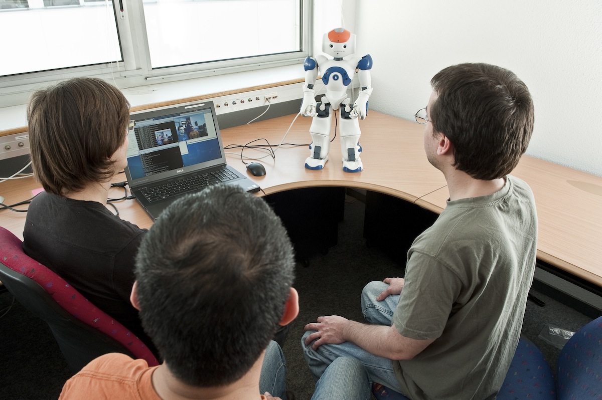
Figure 1: A typical scenario in which a companion humanoid robot (NAO) performs audio-visual fusion in an attempt to assess the auditory status of each one of the speakers in front of the robot and to estimate the 3D locations of their faces. The method uses the robot’s onboard cameras and microphones as well as a modular software architecture based on the freely available RSB (robotics service bus) middleware. This allows untethered interaction between robots and people. Moreover, RSB allows remote algorithm implementation using external computing power and without the performance and deployment restrictions imposed by the onboard computing resources.

The remainder of the paper is organized as follows: Section 2 delineates the related published work, Section 3 outlines the hybrid deterministic/probabilistic model, Section 4 gives the details of the auditory and visual extracted features, Sections 5 and 6 describe the multimodal inference procedure as well as its on-line implementation on the humanoid robot NAO, Section 7 shows the results we obtained and Section 8 draws some conclusions and future work guidelines.

2 Related Work

While vision and hearing have been mainly addressed separately, several behavioral, electrophysiological and imaging studies [Calvert 04], [Ghazanfar 06], [Senkowski 08] postulate that the fusion of different sensorial modalities is an essential component of perception. Nevertheless, computational models of audio-visual fusion and their implementation on robots remain largely unexplored.

The problem of integrating data gathered with physically different sensors, e.g., cameras and microphones, is extremely challenging. Auditory and visual sensor-data correspond to different physical phenomena which must be interpreted in a different way. Relevant visual information must be inferred from the way light is reflected by scene objects and valid auditory information must be inferred from the perceived signals such that it contains the properties of one or several emitters. The spatial and temporal distributions of auditory and visual data are also very different. Visual data are spatially dense and continuous in time. Auditory data are spatially sparse and intermittent since in a natural environment there are only a few acoustic sources. These two modalities are perturbed by different phenomena such as occlusions and self-occlusions (visual data) or ambient noise and echoic environments (auditory data).

Despite all these challenges, numerous researchers investigated the fusion of auditory and visual cues in a variety of domains such as event classification [Natarajan 12], speech recognition [Barker 09], sound source separation [Naqvi 10], speaker tracking [Hospedales 08], [Gatica-Perez 07] and speaker diarization [Noulas 12]. However, these approaches are not suitable for robots either because the algorithmic complexity is too high, or because methods use a distributed sensor network or because the amount of training data needed is too high, drastically reducing the robots’ adatableness. Unfortunately, much less effort has been devoted to design audio-visual fusion methods for humanoid robots. Nevertheless, there are some interesting works introducing methods specifically conceived for humanoid robots on speech recognition [Nakadai 04], beat tracking [Itohara 11], [Itohara 12], active audition [Kim 07] and sound recognition [Nakamura 11]. All these methods deal with the detection and localisation problem by using a combination of off-the-shelf algorithms, suitable for humanoid robots. Albeit, all these approaches lack from a framework versatile enough to be used in other situations than the ones they are specifically designed for.

Finding the potential speakers and assessing their speaking status is a pillar task, on which all applications mentioned above rely. In other words, providing a robust framework to count how many speakers are in the scene, to localize them and to ascertain their speaking state, will definitely increase the performance of many audio-visual perception methods. This problem is particularly interesting in the case of humanoid robots, because the framework must be designed for untethered interaction using a set of robocentric sensors. That is to say that the cameras and microphones are mounted onto a robotic platform that freely interacts with the unconstrained AV events (i.e., people). As a consequence, the use of any kind of distributed sensor network, e.g. close-range microphones and speaker-dedicated cameras, is not appropriated. Likewise, the algorithms should be light enough to satisfy the constraints associated to real-time processing with a humanoid robot.

The existing literature on speaker detection and localisation can be grouped into two main research lines. On one side, many statistical non-parametric approaches have been developed. Indeed, [Gurban 06], [Besson 08b] and [Besson 08a] investigate the use of information theory-based methods to associate auditory and visual data in order to detect the active speaker. Similarly, [Barzelay 07] proposes an algorithm matching auditory and visual onsets. Even though these approaches show very good performance results, they use speaker/object dedicated cameras, thus limiting the interaction. Moreover, the cited non-parametric approaches need a lot of training data. The outcome of such training steps is also environment-dependent. Consequently, implementing such methods on mobile platforms results in systems with almost no practical adaptability.

On the other side, several probabilistic approaches have been published. In [Khalidov 08], [Khalidov 11], the authors introduce the notion of conjugate GMM for audio-visual fusion. Two GMMs are estimated, one for each modality (vision and auditory) while the two mixture parameter sets are constrained through a common set of tying parameters, namely the 3D locations of the AV events being sought. Recently in [Noulas 12], a factorial HMM is proposed to associate auditory, visual and audio-visual features. All these methods simultaneously detect and localize the speakers but they are not suitable for real-time processing, because of their algorithmic complexity. [Kim 07] proposed a Bayesian framework inferring the position of the active speaker and combining a sound source localisation technique with a face tracking algorithm on a robot. The reported results are good in the case of one active speaker, but show bad performance for multiple/far speakers. This is due to the fact that the proposed probabilistic framework is not able to correctly handle outliers. In [Alameda-Pineda 11], the authors use a 1D GMM to fuse the auditory and visual data, building AV clusters. The probabilistic framework is able to handle the outliers thanks to one of the mixture components. However, the algorithm presented in the paper is not light enough for real-time processing.

Unlike these recent approaches, we propose a novel hybrid deterministic/probabilistic model for audio-visual detection and localisation of speaking people. Up to the authors’ knowledge, we introduce the very first model with the following remarkable attributes all together: (i) theoretically sound and solid, (ii) designed to process robocentric data, (iii) accommodating different visual and auditory features, (iv) robust to noise and outliers, (v) requiring a once-and-forever tiny calibration step guaranteeing the adaptability of the system, (vi) working on unrestricted indoor environments, (vii) handling a variable number of people and (viii) implemented on a humanoid platform.

3 A Hybrid Deterministic/Probabilistic Model

We introduce a multimodal deterministic/probabilistic fusion model for audio-visual detection and localisation of speaking people that is suitable for real-time applications. The algorithms derived from that hybrid model aim to count how many speakers are there, find them in the scene and ascertain when they speak. In other words, we seek for the number of potential speakers, $N\in\mathbb{N}$, their positions $\mbox{\boldmath$S$}_{n}\in\mathbb{S}$ ($\mathbb{S}\subset\mathbb{R}^{3}$ is the scene space) and their speaking state $e_{n}\in\{0,1\}$ (0 – not speaking and 1 – speaking).

In order to accomplish the detection and localization of speakers, auditory and visual features are extracted from the raw signals (sound track and image flow), during a time interval $\Delta t$. We assume $\Delta t$ to be short enough such that the speakers remain approximately in the same 3D location and long enough to capture small displacements and oscillatory movements of the head, hands, torso and legs. The auditory and visual features extracted during $\Delta t$ are denoted by $\mbox{\bf a}=\left\{\mbox{\boldmath$a$}_{1},\ldots,\mbox{\boldmath$a$}_{k},\ldots,\mbox{\boldmath$a$}_{K}\right\}\subset\mathbb{A}$ and by $\mbox{\bf v}=\left\{\mbox{\boldmath$v$}_{1},\ldots,\mbox{\boldmath$v$}_{m},\ldots,\mbox{\boldmath$v$}_{M}\right\}\subset\mathbb{V}$ respectively, where $\mathbb{A}$ ($\mathbb{V}$) is the auditory (visual) feature space.

We aim to solve the task from the auditory and visual observations. That is, we want to compute the values of $N$, $\{\mbox{\boldmath$S$}_{n}\}_{n=1}^{N}$ and $\{e_{n}\}_{n=1}^{N}$, that best explain the extracted features a and v. Therefore, we need a framework that encompasses all (hidden and observed) variables and that accounts for the following challenges: (i) the visual and auditory observations lie in physically different spaces with different dimensionality, (ii) the object-to-observation assignments are not known in advance, (iii) both visual and auditory observations are contaminated with noise and outliers, (iv) the relative importance of the two types of data is unassessed, (v) the position and speaking state of the speakers has to be gauged and (vi) since we want to be able to deal with a variable number of AV objects over a long period of time, the number of AV object that are effectively present in the scene must be estimated.

We propose a hybrid deterministic/probabilistic framework performing audio-visual fusion, seeking for the desired variables and accounting for the outlined challenges. On one hand, the deterministic components allow us to model those characteristics of the scene that are known with precision in advance. They may be the outcome of a very accurate calibration step, or the direct consequence of some geometrical or physical properties of the sensors. On the other hand, the probabilistic components model random effects. For example, the feature noise and outliers, which is a consequence of the contents of the scene as well as the feature extraction procedure.

3.1 The Deterministic Model

In this section we delineate the deterministic components of our hybrid model: namely the visual and auditory mappings. Because the scene space, the visual space and the auditory space are different we need two mappings: the first one, ${\cal A}:\mathbb{S}\rightarrow\mathbb{A}$, links the scene space to the auditory space and the second one, ${\cal V}:\mathbb{S}\rightarrow\mathbb{V}$, links the scene space to the visual space. Both mappings are represented in Figure 2. An AV object placed at $S$ in the scene space, is virtually placed at ${\cal A}(\mbox{\boldmath$S$})$ in the auditory space and at ${\cal V}(\mbox{\boldmath$S$})$ in the visual space.

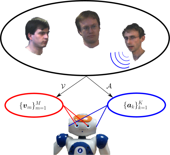
Figure 2: Perceptual auditory ($\cal A$) and visual ($\cal V$) mappings of NAO. The extracted auditory $\mbox{\boldmath$a$}_{k}$ and lay around ${\cal A}(\mbox{\boldmath$S$})$ and ${\cal V}(\mbox{\boldmath$S$})$ respectively. An audio-visual mapping needs to be built to link the two observations spaces.

The definition of ${\cal A}$ and ${\cal V}$ provide a link between the two observations spaces, which corresponds either to ${\cal A}\circ{\cal V}^{-1}$ or to ${\cal V}\circ{\cal A}^{-1}$. Depending on the extracted features and on the sensors, the mappings ${\cal A}$ and ${\cal V}$ may be invertible. If that is not the case, ${\cal A}\circ{\cal V}^{-1}$ or ${\cal V}\circ{\cal A}^{-1}$ should be estimated through a learning procedure. There are several works already published dealing with this problem in different ways. In [Alameda-Pineda 11, Sanchez-Riera 12], ${\cal V}$ is invertible and ${\cal A}$ is known, so building ${\cal A}\circ{\cal V}^{-1}$ is straightforward. In sound source localization approaches (inter alia [Nakadai 04]) ${\cal A}$ is invertible and ${\cal V}$ is known so ${\cal V}\circ{\cal A}^{-1}$ is easily constructed. In [Khalidov 08, Khalidov 11], none of the mappings are inverted, but used to tie the parameters of the probabilistic model. So the link between $\mathbb{A}$ and $\mathbb{V}$ is not used explicitly, but implicitly. In [Butz 05, Kidron 05, Kidron 07, Liu 08], the scene space is undetermined and the authors learn a common representation space (the scene space) at the same time they learn both mappings.

In our case, we chose to extract 3D visual feature points, and represent them in the scene coordinate system (see Section 4.2). Thus, the mapping ${\cal V}$ is the identity, which is invertible. The auditory features correspond to the Interaural Time Differences (see Section 4.1), and a direct path propagation model defines ${\cal A}$. The mapping ${\cal A}\circ{\cal V}^{-1}$ is accurately built from the geometric and physical models estimated through a calibration step (see Section 4.3). Consequently, we are able to map the visual features $\mbox{\bf v}=\{\mbox{\boldmath$v$}_{1},\ldots,\mbox{\boldmath$v$}_{M}\}$ onto the auditory space $\mathbb{A}$. We will denote the projection of $\mbox{\boldmath$v$}_{m}$ by $\tilde{\mbox{\boldmath$v$}}_{m}$:

$$\tilde{\mbox{\boldmath$v$}}_{m}=({\cal A}\circ{\cal V}^{-1})(\mbox{\boldmath$v$}_{m}).$$

Summarizing, we use the mapping from $\mathbb{V}$ to $\mathbb{A}$ to map all visual features onto the auditory space. Hence, all extracted features lie, now, in the same space, and we can perform the multimodal fusion in there.

3.2 The Probabilistic Model

Thanks to the link built in the previous section, we obtain a set of projected visual features $\tilde{\mbox{\bf v}}=\{\tilde{\mbox{\boldmath$v$}}_{1},\ldots,\tilde{\mbox{\boldmath$v$}}_{M}\}$, laying in the same space as the auditory features a. These features need to be grouped to construct audio-visual objects. However, we do not know which observation is generated by which object. Therefore, we introduce two sets of hidden variables $Z$ and $W$:

$$Z = \{Z_{1},\ldots,Z_{m},\ldots,Z_{M}\}$$

$$W = \{W_{1},\ldots,W_{k},\ldots,W_{K}\},$$

accounting for the observation-to-object assignment. The notation $Z_{m}=n$ ($m\in\{1,\ldots,M\}$, $n\in\{1,\ldots,N+1\}$) means that the projected visual observation $\tilde{\mbox{\boldmath$v$}}_{m}$ was either generated by the $n^{\textrm{th}}$ 3D object ($n\in\{1,\ldots,N\}$) or it is an outlier ($n=N+1$). Similarly, the variable $W_{k}$ is associated to the auditory observation $\mbox{\boldmath$a$}_{k}$.

We formulate the multimodal probabilistic fusion model under the assumption that all observations $\tilde{\mbox{\boldmath$v$}}_{m}$ and $\mbox{\boldmath$a$}_{k}$ are independent and identically distributed. The $n^{\textrm{th}}$ AV object generates both visual and auditory features normally distributed around ${\cal A}(\mbox{\boldmath$S$}_{n})$ and both the visual and auditory outliers are uniformly distributed in $\mathbb{A}$. Therefore, we write:

$$\textrm{P}(\tilde{\mbox{\boldmath$v$}}_{m}|Z_{m}=n,\Theta)=\left\{\begin{array}[]{ll}{\cal N}(\tilde{\mbox{\boldmath$v$}}_{m};\mu_{n},\sigma_{n})&n=1,\ldots,N\\ {\cal U}(\tilde{\mbox{\boldmath$v$}}_{m};\mathbb{A})&n=N+1\\ \end{array}\right..$$

where $\Theta$ contains the Gaussian parameters, that is $\mu_{n}={\cal A}(\mbox{\boldmath$S$}_{n})$ and $\sigma_{n}$ (the mean and the standard deviation of the $n^{\textrm{th}}$ Gaussian). The exact same rule holds for $\textrm{P}(\mbox{\boldmath$a$}_{m}|W_{m}=n,\Theta)$. Thus we can define a generative model for the observations $x\in\mathbb{A}$:

$$\textrm{p}\left(x;\Theta\right)=\sum_{n=1}^{N}\pi_{n}\,{\cal N}(x;\mu_{n},\sigma_{n})+\pi_{N+1}\,{\cal U}(x;\mathbb{A}),$$ (1)

where $\pi_{n}$ is the prior probabilities of the $n^{\textrm{th}}$ mixture component. That is, $\pi_{n}=\textrm{P}(Z_{m}=n)=\textrm{P}(W_{k}=n)$, $\forall n,m,k$. The prior probabilities satisfy $\sum_{n=1}^{N+1}\pi_{n}=1$. Summarizing, the model parameters are:

$$\Theta=\{\pi_{1},\ldots,\pi_{N+1},\mu_{1},\ldots,\mu_{N},\sigma_{1},\ldots,\sigma_{N}\}.$$ (2)

Under the probabilistic framework described, the set of parameters is estimated within a maximum likelihood formulation:

$${\cal L}\left(\tilde{\mbox{\bf v}},\mbox{\bf a};\Theta\right)=\sum_{m=1}^{M}\log\textrm{p}\left(\tilde{\mbox{\boldmath$v$}}_{m};\Theta\right)+\sum_{k=1}^{K}\log\textrm{p}\left(\mbox{\boldmath$a$}_{k};\Theta\right).$$ (3)

In other words, the optimal set of parameters is the one maximizing the log-likelihood function (3), where p is the generative probabilistic model in (1). Unfortunately, direct maximization of (3) is an intractable problem. Equivalently, the expected complete-data log-likelihood will be maximized [Dempster 77] (see Section 5).

We recall that the ultimate goal is to determine the number $N$ of AV events, their 3D locations $\mbox{\boldmath$S$}_{1},\ldots,\mbox{\boldmath$S$}_{n},\ldots,\mbox{\boldmath$S$}_{N}$ as well as their auditory activity $e_{1},\ldots,e_{n},\ldots,e_{N}$. However, the 3D location parameters can be computed only indirectly, once the multimodal mixture’s parameters $\Theta$ have been estimated. Indeed, once the auditory and visual observations are grouped in $\mathbb{A}$, the $\tilde{\mbox{\boldmath$v$}}_{m}\leftrightarrow\mbox{\boldmath$v$}_{m}$ correspondences are used to infer the locations $\mbox{\boldmath$S$}_{n}$ of the AV objects and the grouping of the auditory observations a is used to infer the speaking state $e_{n}$ of the AV objects. The choice of $N$ as well as the formulas for $\mbox{\boldmath$S$}_{n}$ and $e_{n}$ are given in Sections 5.2 and 5.3 respectively. Before these details are given and in order to fix ideas, we devote next section to describe the auditory and visual features, justify the existence of ${\cal V}^{-1}$ and detail the calibration procedure leading to a highly accurate mapping ${\cal A}\circ{\cal V}^{-1}$.

4 Finding Auditory and Visual Features

In this section we describe the auditory (Section 4.1) and the visual (Section 4.2) features we extract from the raw data. Given this features, the definition of ${\cal A}$ and ${\cal V}$ is straightforward. However, the computation of the mapping’s parameters is done through a calibration procedure detailed in Section 4.3.

4.1 Auditory Features

An auditory observation $\mbox{\boldmath$a$}_{k}$ corresponds to an Interaural Time Difference (ITD) between the left and right microphones. Because the ITDs are real-valued, the auditory feature space is $\mathbb{A}=\mathbb{R}$. One ITD value corresponds to the different of time of arrival of the sound signal between the left and right microphones. For instance, the sound wave of a speaker located in the left-half of the scene will obviously arrive earlier to the left microphone than to the right microphone. We found that the method proposed in [Christensen 07] yields very good results that are stable over time. The relationship between an auditory source located at $\mbox{\boldmath$S$}\in\mathbb{R}^{3}$ and an ITD observation $a$ depends on the relative position of the acoustic source with respect to the locations of the left and right microphones, $\mbox{\boldmath$M$}_{L}$ and $\mbox{\boldmath$M$}_{R}$. If we assume direct sound propagation and constant sound velocity $\nu$, this relationship is given by the mapping ${\cal A}:\mathbb{S}\rightarrow\mathbb{A}$ defined as:

$${\cal A}(\mbox{\boldmath$S$})=\frac{\|\mbox{\boldmath$S$}-\mbox{\boldmath$M$}_{L}\|-\|\mbox{\boldmath$S$}-\mbox{\boldmath$M$}_{R}\|}{\nu}.$$ (4)

4.2 Visual Features

The visual observations are 3D points extracted using binocular vision. We used two types of features: the Harris-Motion 3D (HM3D) points and the faces 3D (F3D).

HM3D

The first kind of features we extracted are called Harris-motion points. We first detect Harris interest points [Harris 88] in the left and right image pairs of the time interval $\Delta t$. Second, we only consider a subset of theses points, namely those points where motion occurs. For each interest-point image location $(u,v)$ we consider the image intensities at the same location $(u,v)$ in the subsequent images and we compute a temporal intensity standard deviation $\tau_{(u,v)}$ for each interest point. Assuming stable lighting condition over $\Delta t$, we simply classify the interest points into static ($\tau_{(u,v)}\leq\tau_{M}$) and dynamic ($\tau_{(u,v)}>\tau_{M}$) where $\tau_{M}$ is a user-defined threshold. Third, we apply a standard stereo matching algorithm and a stereo reconstruction algorithm [Hartley 04] to yield a set of 3D features v associated with $\Delta t$.

F3D

The second kind of features are the 3D coordinates of the speakers’ faces. They are obtained using the face detector in [Šochman 05]. More precisely, the center of the bounding box retrieved by the face detector is matched to the right image and the same stereo reconstruction algorithm as in HM3D is used to obtain v.

Both 3D features are expressed in cyclopean coordinates [Hansard 08], which are also the scene coordinates. Consequently, the visual mapping ${\cal V}$ is the identity mapping. In conclusion, because we are able to accurately model the geometry of the visual sensors, we can assume that ${\cal V}$ is invertible and explicitly build the linking mapping ${\cal A}\circ{\cal V}^{-1}$.

4.3 Calibration

In the two previous sections we described the auditory and the visual features respectively. As a consequence, the mappings ${\cal A}$ and ${\cal V}$ are defined. However, we made implicit use of two, a priory unknown, objects. On one hand the stereo-matching and the 3D reconstruction algorithms need the so-called stereo-calibration. That is, the projection matrices corresponding to the left and right cameras which are estimated using [Bouguet 08]. It is worth to remark that the calibration procedure allows us to accurately represent any point in the field-of-view of both cameras as a 3D point. On the other hand, and in order to use ${\cal A}$, we need to know the positions of the microphones $\mbox{\boldmath$M$}_{L}$ and $\mbox{\boldmath$M$}_{R}$ in the scene coordinate frame, which is slightly more complex. Since the scene coordinates are the same as the visual coordinates, we refer to this as “audio-visual calibration”. We manually measure the values of $\mbox{\boldmath$M$}_{L}$ and $\mbox{\boldmath$M$}_{R}$ with respect to the stereo rig. However, because these measurements are imprecise, an affine correction model needs to be applied:

$$\overline{\cal A}(\mbox{\boldmath$S$})=c_{1}\,{\cal A}(\mbox{\boldmath$S$})+c_{0}=c_{1}\,\frac{\|\mbox{\boldmath$S$}-\mbox{\boldmath$M$}_{L}\|-\|\mbox{\boldmath$S$}-\mbox{\boldmath$M$}_{R}\|}{\nu}+c_{0},$$ (5)

where $c_{1}$ and $c_{0}$ are the adjustment coefficients. In order to estimate $c_{1}$ and $c_{0}$, a person with a speaker held just below the face moves in a zig-zag trajectory in the entire visual field of view of the two cameras. The 3D position of the person’s face and the ITD values were extracted. We used white noise because it correlates very well resulting in a single sharp peak in ITD space. In many experiments, we did not observe any effect of reverberations, because the reverberant components are suppressed by the direct component of the long lasting white noise signal. The optimal values for $c_{1}$ and $c_{0}$, in the least square sense, were computed from these data. Figure 3 shows the extracted ITDs (red-circle), the projected faces before (blue) and after (green) the affine correction. We can clearly see how the affine transformation enhanced the audio-visual linking mapping. Hence the projected visual features have the following expression:

$$\tilde{\mbox{\boldmath$v$}}_{m}=(\overline{\cal A}\circ{\cal V}^{-1})(\mbox{\boldmath$v$}_{m})=c_{1}\,\frac{\|\mbox{\boldmath$v$}_{m}-\mbox{\boldmath$M$}_{L}\|-\|\mbox{\boldmath$v$}_{m}-\mbox{\boldmath$M$}_{R}\|}{\nu}+c_{0}.$$ (6)

The outlined calibration procedure has three main advantages: (i) it requires very few training data, (ii) it lasts a long period of time and (iii) it is environment-independent, thus guaranteeing the system’s adaptability. Indeed, in our case, the calibration ran on a one-minute audio-visual sequence and has been successfully used for the last 18 months in several rooms, including project demonstrations and conference exhibits. Consequently, the robustness of the once-for-all tiny audio-visual calibration step is proved up to a large extent.

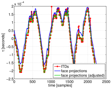
Figure 3: Affine correction of the audio-visual calibration. Extracted ITD values are plot in red-circled. F3D features projected into the ITD space using Equation (4) are plot in blue. F3D features projected using Equation (6), that is after the audio-visual calibration step, are plot in green.

5 Multimodal Inference

In Section 3 we set up the maximum-likelihood framework to perform AV fusion. The 3D visual features are mapped into the auditory space $\mathbb{A}$ through the audio-visual mapping $(\overline{\cal A}\circ{\cal V}^{-1})$. This mapping takes the form in (6) when using the auditory and visual features described in Section 4. However, three of the initial issues remain unsolved: (i) the relative importance of each modality, (ii) the estimates for $\mbox{\boldmath$S$}_{n}$ and $e_{n}$ and (iii) the variable number of AV objects, $N$. In this Section we described EM-based method solving the ML problem with hidden variables and accounting for these unsolved issues.

5.1 Visual guidance

Previous papers do not agree on how to balance the relative importance of each modality. After a deep analysis of the features’ statistics, we choose to use the visual information to guide the clustering process of the sparse auditory observations. Indeed, because the HM3D visual features are more dense and have better temporal continuity than the ITD values, we start by fitting a 1D GMM to the projected visual features $\{\tilde{\mbox{\boldmath$v$}}_{m}\}_{m=1}^{M}$. This is done with the standard EM algorithm [Bishop 06]. In the E step of the algorithm the posterior probabilities $\alpha_{mn}=\textrm{P}(Z_{m}=n|\tilde{\mbox{\bf v}},\Theta)$ are updated via the following formula:

$$\alpha_{mn}=\frac{\pi_{n}\,\textrm{P}(\tilde{\mbox{\boldmath$v$}}_{m}|Z_{m}=n,\Theta)}{\sum_{i=1}^{N+1}\pi_{i}\,\textrm{P}(\tilde{\mbox{\boldmath$v$}}_{m}|Z_{m}=i,\Theta)}.$$ (7)

The M step is devoted to maximize the expected complete data log-likelihood with respect to the parameters, leading to the standard formulas (with $\bar{\alpha}_{n}=\sum_{m=1}^{M}\alpha_{mn}$):

$$\pi_{n} = \frac{\bar{\alpha}_{n}}{M},$$

$$\mu_{n} = \frac{1}{\bar{\alpha}_{n}}\sum_{m=1}^{M}\alpha_{mn}\tilde{\mbox{\boldmath$v$}}_{m},$$

$$\sigma_{n}^{2} = \frac{1}{\bar{\alpha}_{n}}\sum_{m=1}^{M}\alpha_{mn}(\tilde{\mbox{\boldmath$v$}}_{m}-\mu_{n})^{2}.$$

Once the model is fitted to the projected visual data, i.e., the visual information has already been probabilistically assigned to the $N$ objects, the clustering process proceeds by including the auditory information. Hence, we are faced with a constrained maximum-likelihood estimation problem: maximize (3) subject to the constraint that the posterior probabilities $\alpha_{mn}$ were previously computed. This leads to vision-guided EM fusion algorithm in which the E-step only updates the posterior probabilities associated with the auditory observations while those associated with the visual observations remain unchanged. This semi-supervision strategy was introduced in the context of text classification [Nigam 00, Miller 03]. Here it is applied to enforce the quality and reliability of one of the sensing modalities within a multimodal clustering algorithm. To summarize, the E-step of the algorithm updates only the posterior probabilities of the auditory observations $\beta_{kn}=\textrm{P}(W_{k}=n|\mbox{\bf a},\Theta)$:

$$\beta_{kn}=\frac{\pi_{n}\,\textrm{P}(\mbox{\boldmath$a$}_{k}|W_{k}=n,\Theta)}{\sum_{i=1}^{N+1}\pi_{i}\,\textrm{P}(\mbox{\boldmath$a$}_{k}|W_{k}=i,\Theta)},$$ (8)

while keeping the visual posterior probabilities, $\alpha_{mn}$, constant. The M-step has a closed-form solution and the prior probabilities are updated with:

$$\pi_{n}=\frac{\gamma_{n}}{M+K},\quad n=1,\ldots,N+1,$$

with $\gamma_{n}=\sum_{m=1}^{M}\alpha_{mn}+\sum_{k=1}^{K}\beta_{kn}=\bar{\alpha}_{n}+\bar{\beta}_{n}$. The means and variances of the current model are estimated by combining the two modalities:

$$\mu_{n}=\frac{1}{\gamma_{n}}\left(\sum_{m=1}^{M}\alpha_{mn}\,\tilde{\mbox{\boldmath$v$}}_{m}+\sum_{k=1}^{K}\beta_{kn}\,\mbox{\boldmath$a$}_{k}\right),$$ (9)

$$\sigma^{2}_{n}=\frac{\sum_{m=1}^{M}\alpha_{mn}\,(\tilde{\mbox{\boldmath$v$}}_{m}-\mu_{n})^{2}+\sum_{k=1}^{K}\beta_{kn}\,(\mbox{\boldmath$a$}_{k}-\mu_{n})^{2}}{\gamma_{n}}.$$ (10)

5.2 Counting the number of speakers

Since we do not know the value of $N$, a reasonable way to proceed is to estimate the parameters $\Theta_{N}$ for different values of $N$ using the method delineated in the previous section. Once we estimated the maximum likelihood parameters for models with different number of AV objects, we need a criterion to choose which is the best one. This is estimating the number of AV objects (clusters) in the scene. BIC [Schwarz 78] is a well known criterion to choose among several maximum likelihood statistical models. BIC is often chosen for this type of tasks due to its attractive consistency properties [Keribin 00]. It is appropriate to use this criterion in our framework, due to the fact that the statistical models after the vision-guided EM algorithm, fit the AV data in an ML sense. In our case, choosing among these models is equivalent to estimate the number of AV events $\hat{N}$. The formula to compute the BIC score is:

$$\textrm{BIC}(\tilde{\mbox{\boldmath$v$}},\mbox{\bf a},\Theta_{N})={\cal L}\left(\tilde{\mbox{\boldmath$v$}},\mbox{\bf a};\Theta_{N}\right)-\frac{D_{N}\,\log(M+K)}{2},$$ (11)

where $D_{N}=3N$ is the number of free parameters of the model.

The number of AV events is estimated by selecting the statistical model corresponding to the maximum score:

$$\hat{N}=\arg\max\limits_{N}\textrm{BIC}(\tilde{\mbox{\boldmath$v$}},\mbox{\bf a},\Theta_{N}).$$ (12)

5.3 Detection and localisation

The selection on $N$ leads to the best maximum-likelihood model in the BIC sense. That is, the set of parameters that best explain the auditory and visual observations a and $\tilde{\mbox{\bf v}}$. In the following, v are used to estimate the 3D positions in the scene and a to estimate the speaking state of each AV object.

The locations of the AV objects are estimated thanks to the one-to-one correspondence between 3D visual features and the 1D projected features, $\tilde{\mbox{\boldmath$v$}}_{m}\leftrightarrow\mbox{\boldmath$v$}_{m}$. Indeed, the probabilistic assignments of the projected visual data onto the 1D clusters, $\alpha_{mn}$, allow us to estimate $\mbox{\boldmath$S$}_{n}$ through:

$$\hat{\mbox{\boldmath$S$}}_{n}=\frac{1}{\bar{\alpha}_{n}}\sum_{m=1}^{M}\alpha_{mn}\mbox{\boldmath$v$}_{m}.$$ (13)

The auditory activity associated to the $n^{\textrm{th}}$ speaker is estimated as follows ($\tau_{A}$ is a user-defined threshold):

$$\hat{e}_{n}=\left\{\begin{array}[]{ll}1&\mbox{if }\bar{\beta}_{n}>\tau_{A}\\ 0&\mbox{otherwise}\end{array}\right.$$ (14)

This two formulas account for the last remaining issue: the 3D localization and speaking state estimation of the AV objects. Next section describes some practical considerations to take into account when using this EM-based AV fusion method. Afterward, in Section 5.5, we summarize the method by providing an algorithmic scheme of the multimodal inference procedure.

5.4 Practical Concerns

Even though the EM algorithm has proved to be the proper (and extremely powerful) methodology to solve ML problems with hidden variables, in practice we need to overcome two main hurdles. First, since the log-likelihood function has many local maxima and EM is a local optimization technique, a very good initialization is required. Second, because real data is finite and may not strictly follow the generative law of probability (1), the consistency properties of the EM algorithm do not guarantee that the model chosen by BIC is meaningful regarding the application. Thus, a post-processing step is needed in order to include the application-dependant knowledge. In all, we must account for three practical concerns: (i) EM initialization, (ii) eventual shortage of observations and (iii) the probabilistic model does not fully correspond to the observations.

It is reasonable to assume that the dynamics of the AV objects are somehow constrained. In other words, the positions of the objects at a time interval are close to the positions at the previous time interval. Hence, we use the model computed in the previous time interval to initialize the EM based procedure. More precisely, if we denote by $N^{(p)}$ the number of AV objects found in the previous time interval, we initialize a new 1D GMM with $N$ clusters, for $N\in\{0,\ldots,N_{\textrm{max}}\}$. In the case $N\leq N^{(p)}$, we take the $N$ clusters with the highest weight. For $N>N^{(p)}$, we incrementally split a cluster at its mean into two clusters. The cluster to be split is selected on the basis of a high Davies-Bouldin index [Davies 79]:

$$DW_{i}=\max_{j\neq i}\frac{\sigma_{i}+\sigma_{j}}{\|\mu_{i}-\mu_{j}\|}.$$

We chose to split the cluster into two clusters in order to detect AV objects that have recently appeared in the scene, either because they were outside the field of view, or because they were occluded by another AV object. This provides us with a good initialization. In our case the maximum number of AV objects is $N_{\textrm{max}}=10$.

A shortage of observations usually leads to clusters whose interactions may describe an overall pattern, instead of different components. We solve this problem by merging some of the mixture’s components. There are several techniques to merge clusters within a mixture model (see [Hennig 10]). Since the components to be merged lie around the same position and have similar spread, the ridgeline method [Ray 05] best solves our problem.

Finally, we need to face the fact that the probabilistic model does not fully represent the observations. Indeed, we observed the existence of spurious clusters. Although the 3D visual observations associated with these clusters may be uniformly distributed, their projections onto the auditory space $\tilde{\mbox{\boldmath$v$}}_{m}$ may form a spurious cluster. Hence these clusters are characterized by having their points distributed near some hyperboloid in the 3D space (hyperboloids are the level surfaces of the linking mapping defined in (6)). As a consequence, the volume of the back-projected 3D cluster is small. We discard those clusters whose covariance matrix has a small determinant. Similarly as in (15), the clusters’ covariance matrix is estimated via:

$$\hat{{\bf\Sigma}}_{n}=\frac{1}{\bar{\alpha}_{n}}\sum_{m=1}^{M}\alpha_{mn}\left(\mbox{\boldmath$v$}_{m}-\hat{\mbox{\boldmath$S$}}_{n}\right)\left(\mbox{\boldmath$v$}_{m}-\hat{\mbox{\boldmath$S$}}_{n}\right)^{\top}.$$ (15)

5.5 Motion-Guided Robot Hearing

Algorithm 1 below summarizes the proposed method. It takes as input the visual (MH3D) and auditory (ITD) observations gathered during a time interval $\Delta t$. The algorithm’s output is the estimated number of clusters $\hat{N}$, the estimated 3D positions of the AV events $\{\hat{\mbox{\boldmath$S$}}_{n}\}_{n=1}^{\hat{N}}$ as well as their estimated auditory activity $\{\hat{e}_{n}\}_{n=1}^{\hat{N}}$. Because the grouping process is supervised by the HM3D features, we name the procedure Motion-Guided Robot Hearing. The algorithm starts by mapping the visual observations onto the auditory space by means of the linking mapping defined in (6). Then, for $N\in\{1,\ldots,N_{\textrm{max}}\}$ it iterates through the following steps: (a) Initialize a model with $N$ components using the output of the previous time interval (Section 5.4), (b) apply EM using the selected $N$ to model the 1D projections of the visual data (Section 5.1), (c) apply the vision-guided EM fusion algorithm to both the auditory and projected visual data (Section 5.1) in order to perform audio-visual clustering, and (d) compute the BIC score associated with the current model, i.e., (11). This allows the algorithm to select the model with the highest BIC score, i.e., (12). The post-processing step is then applied to the selected model (Section 5.4) prior to computing the final output (Section 5.3).

Algorithm 1 Motion-Guided Robot Hearing

1:  Input: HM3D, $\left\{\mbox{\boldmath$v$}_{m}\right\}_{m=1}^{M}$, and ITD, $\left\{\mbox{\boldmath$a$}_{k}\right\}_{k=1}^{K}$, features.

2:  Output: Number of AV events $\hat{N}$, 3D localization $\left\{\hat{\mbox{\boldmath$S$}}_{n}\right\}_{n=1}^{\hat{N}}$ and auditory status $\left\{\hat{e}_{n}\right\}_{n=1}^{\hat{N}}$.

3:  Map the visual features onto the auditory space, $\tilde{\mbox{\boldmath$v$}}_{m}=(\overline{\cal A}\circ{\cal V}^{-1})(\mbox{\boldmath$v$}_{m})$ (6).

4:  for $N=1\to N_{\textrm{max}}$ do

5:     (a) Initialize the model with $N$ clusters (Section 5.4).

6:     (b) Apply EM clustering to $\{\tilde{\mbox{\boldmath$v$}}_{m}\}_{m=1}^{M}$ (Section 5.1).

7:     (c) Apply the Vision-guided EM fusion algorithm to cluster the audio-visual data (Section 5.1).

8:     (d) Compute the BIC score (11).

9:  end for

10:  Estimate the number of clusters based on the BIC score (12).

11:  Post-processing (Section 5.4).

12:  Compute the final outputs $\{\hat{\mbox{\boldmath$S$}}_{n}\}_{n=1}^{\hat{N}}$ and $\{\hat{e}_{n}\}_{n=1}^{\hat{N}}$ (Section 5.3).

6 Implementation on NAO

The previous multimodal inference algorithm has desirable statistical properties and good performance (see Section 7). Since our final aim is to have a stable component working on a humanoid robot (i.e., able to interact with other components), we reduced the computational load of the AV fusion algorithm. Indeed, we adapted the method described in Section 5 to achieve a light on-line algorithm working on mobile robotic platforms.

In order to reduce the complexity, we substituted the Harris-Motion 3D point detector (HM3D) with the face 3D detector (F3D), described in Section 4.2. F3D replaces hundreds of HM3D points with a few face locations in 3D, $\{\mbox{\boldmath$v$}_{m}\}_{m=1}^{M}$. We then consider that the potential speakers correspond to the detected faces. Hence we set $N=M$ and $\mbox{\boldmath$S$}_{n}=\mbox{\boldmath$v$}_{n}$, $n=1,\ldots,N$. This has several crucial consequences. First, the number of AV objects corresponds to the number of detected faces; the model selection step is not needed and the EM algorithm does not have to run $N_{\textrm{max}}$ times, but just once. Second, because the visual features provide a good initialization for the EM (by setting $\mu_{n}=(\overline{\cal A}\circ{\cal V}^{-1})(\mbox{\boldmath$S$}_{n})$), the visual EM is not required and the hidden variables $Z$ do not make sense anymore. Third, since the visual features are not used as observations in the EM, but to initialize it, the complexity of the vision-guide EM fusion algorithm is ${\cal O}(NK)$ instead of ${\cal O}\left(N(K+M)\right)$. This important because the number of HM3D points is much bigger than the number of ITD values, i.e., $M\gg K$. Last, because the visual features provide the $\mbox{\boldmath$S$}_{n}$’s, there is not need to estimate them through (15).

6.1 Face-Guided Robot Hearing

The resulting procedure is called Face-Guided Robot Hearing and it is summarized in Algorithm 2 below. It takes as input the detected heads ($\mbox{\boldmath$S$}_{1},\ldots,\mbox{\boldmath$S$}_{N}$) and the auditory (a) observations gathered during a time interval $\Delta t$. The algorithm’s output is the estimated auditory activity $\{\hat{e}_{n}\}_{n=1}^{N}$.

Algorithm 2 Face-Guided Robot Hearing

1:  Input: Faces’ position $\{\mbox{\boldmath$S$}_{n}\}_{n=1}^{N}$ and auditory $\left\{\mbox{\boldmath$a$}_{k}\right\}_{k=1}^{K}$ features.

2:  Output: AV objects’ auditory status $\left\{\hat{e}_{n}\right\}_{n=1}^{\hat{N}}$.

3:  Map the detected heads onto the auditory space, $\mu_{n}=(\overline{\cal A}\circ{\cal V}^{-1})(\mbox{\boldmath$S$}_{n})$ (6).

4:  Apply EM clustering to $\{\mbox{\boldmath$a$}_{k}\}_{k=1}^{K}$ (Section 5.1).

5:  Compute the final outputs $\{\hat{e}_{n}\}_{n=1}^{\hat{N}}$ (Section 5.3).

6.2 System Architecture

We implemented our method using several components which are connected by a middleware called Robotics Services Bus (RSB) [Wienke 11]. RSB is a platform-independent event-driven middleware specifically designed for the needs of distributed robotic applications. It is based on a logically unified bus which can span over several transport mechanisms like network or in-process communication. The bus is hierarchically structured using scopes on which events can be published with a common root scope. Through the unified bus, full introspection of the event flow between all components is easily possible. Consequently, several tools exist which can record the event flow and replay it later, so that application development can largely be done without a running robot. RSB events are automatically equipped with several timestamps, which provide for introspection and synchronization abilities. Because of these reasons RSB was chosen instead of NAO’s native framework NAOqi and we could implement and test our algorithm remotely without performance and deployment restrictions imposed by the robot platform. Moreover, the resulting implementation can be reused for other robots.

One tool available in the RSB ecosystem is an event synchronizer, which synchronizes events based on the attached timestamps with the aim to free application developers from such a generic task. However, several possibilities of how to synchronize events exist and need to be chosen based on the intended application scenario. For this reason, the synchronizer implements several strategies, each of them synchronizing events from several scopes into a resulting compound event containing a set of events from the original scopes. We used two strategies for the implementation. The ApproximateTime strategy is based on the algorithm available in [ROS 12] and outputs sets of events containing exactly one event from each scope. The algorithm tries to minimize the time between the earliest and the latest event in each set and hence well-suited to synchronize events which originate from the same source (in the world) but suffered from perception or processing delays in a way that they have non-equal timestamps. The second algorithm, TimeFrame, declares one scope as the primary event source and for each event received here, all events received on other scopes are attached that lie in a specific time frame around the timestamp of the source event.

ApproximateTime is used in our case to synchronize the results from the left and right camera as frames in general form matching entities but due to independent grabbing of both cameras have slightly different timestamps. Results from the stereo matching process are synchronized with ITD values using the TimeFrame strategy because the integration time for generating ITD values is much smaller than for a vision frame and hence multiple ITD values belong to a single vision result.

6.3 Modular Structure

The implementation is divided into components shown in the pipeline of Figure 6. Components are color-coded: modules provided by the RSB middleware (white), auditory (red) and visual (green) processing, audio-visual fusion (purple) and the visualization tool (blue) described at the end of this Section.

The visual processing is composed by five modules. Left video and Right video stream the images received at left and right cameras. The Left face detection module extracts the faces from the left image. These are then synchronized with the right image in Face-image synchronization, using the ApproximateTime strategy. The F3D Extraction module computes the F3D features. A new audio-visual head for NAO was used for this implementation. The new head (see Figure 4) is equipped with a pair of cameras and four microphones, thus providing a synchronized VGA stereoscopic image flow as well as four audio channels.

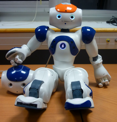
Figure 4: Within this work we used a new audio-visual head that is composed of a synchronized camera pair and two microphones. This “orange” head replaces the former “blue” head and is fully interfaced by the RSB middleware previously described in this section.

The auditory component consists of three modules. Interleaved audio samples coming from the four microphones of NAO are streamed by the Interleaved audio module. The four channels are deinterleaved by the Sound deinterleaving module, which outputs the auditory flows corresponding to the left and right microphones. These flows are stored into two circular buffers in order to extract the ITD values (ITD extraction module).

Both visual and auditory features flow until the Audio-visual synchronization module; the TimeFrame strategy is used here to find the ITD values coming from the audio pipeline associated to the 3D positions of the faces coming from the visual processing. These synchronized events feed the Face-guided robot hearing module, which is in charge of estimating the speaking state of each face, $e_{n}$.

Finally, we developed the module Visualization, in order to get a better insight of the proposed algorithm. A snapshot of this visualization tool can be seen in Figure 5. The image consists of three parts. The top-left part with a blue frame is the original left image plus one rectangle per detected face. In addition to the face’s bounding box, a solid circle is plot on the face of the actor codding the emitting sound probability, the higher it is, the darker the circle. The top-right part, framed in green, is a bird-view of the scene, in which the detected heads appear as circles. The bottom-left part, with a red frame, represents the ITD space. There, both the mapped heads (ellipses) and the histogram of ITD values are plot.

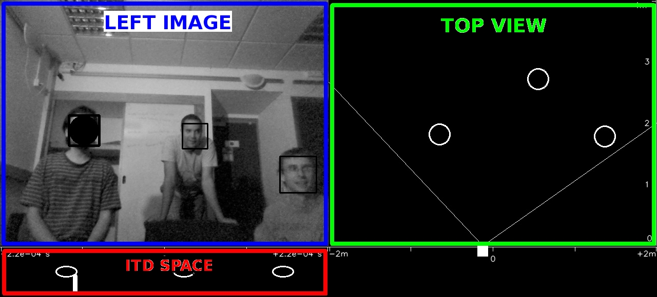
Figure 5: Snapshot of the visualization tool. The top-left (blue-framed) image is the original left image plus one bounding box per detected face. In addition, an intensity-coded circle appears when the speaker is active. The darker the color is, the higher the speaking probability is. The top-right (green-framed) image corresponds to the bird-view of the scene, in which each circle corresponds to a detected head. The bottom-left (red-framed) image represents the ITD space. The projected faces are represented by an ellipse and the histogram of extracted ITD values is plot.

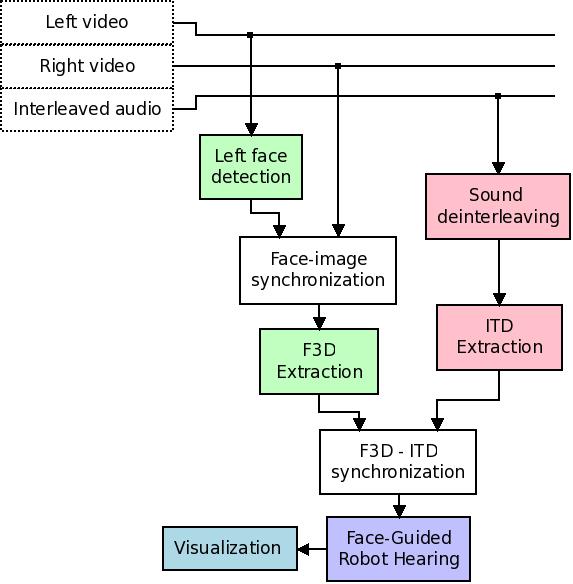
Figure 6: Modular structure of the Face-Guided Robot Hearing procedure implemented on NAO. There are five types of modules: streaming & synchronization (white), visual processing (green), auditory processing (red), audio-visual fusion (purple) and visualization (blue).

6.4 Implementation Details

Some details need to be specified regarding the implementation of the face-guided robot hearing method. First, the integration window $F$ and the frame shift $f$ of the ITD extraction procedure. The bigger the integration window is the more reliable the ITD values are and the more expensive its computation becomes. Similarly, the smaller $f$ is the more ITD observations are extracted and the more computational load we have. A good compromise between low computational load, high rate, and reliability of ITD values was found for $W=150$ ms and $f=20$ ms. We also used an activity threshold: when the energy of the sound signals is lower than $E_{A}=0.001$, the window is not processed. Thus saving computational time for other components in the system when there are no emitted sounds. Notice that this parameter could be controlled by a higher level module which would learn the characteristics of the scene and infer the level of background noise. We initialize $\sigma_{n}^{2}=10^{-9}$, since we found this value big enough to take into account the noise in the ITD values and small enough to discriminate speakers that are close to each other. The threshold $\tau_{A}$ has to take into account how many audio observations ($K$) are gathered during the current time interval $\Delta t$ as well as the number of potential audible AV objects ($N$). For instance, if there is just one potential AV object, most of the audio observations should be assigned to it, whereas if there are three of them the audio observations may be distributed among them (in case all of them emit sounds). The threshold $\tau_{A}$ was experimentally set to $\tau_{A}=K/(N+2)$. The entire pipeline was running on a laptop with an i7 processor at $2.5$ GHz.

7 Results

In order to evaluate the proposed approach, we ran three sets of experiments. First, we evaluated the Multimodal Inference method described in Section 5 on synthetic data. This allowed us to assess the quality of the model on a controlled scenario, where the feature extraction did not play any role. Second, we evaluated the Motion-Guided Robot Hearing method on a publicly available dataset, thus assessing the quality of the entire approach. Finally, we evaluated the Face-Guided Robot Hearing implemented on NAO, which proves that the proposed hybrid deterministic/probabilistic framework is suitable for robot applications.

In all our experiments we used a time interval of 6 visual frames, $\Delta t=0.4s$; time in which approximately 2,000 HM3D observations and 20 auditory observations are extracted. A typical set of visual and auditory observations are shown in Figures 7 and 8. Indeed, Figure 7 focuses on the extraction of the HM3D features: the Harris interest point detection, filtered by motion, matched between images and reconstructed in 3D. Figure 8 shows the very same 3D features projected in to the ITD space. Also, the ITD values extracted during the same time interval are shown. These are the input features of the Motion-Guided Robot Hearing procedure. Notice that both auditory and visual data are corrupted by noise and by outliers. Visual data suffer from reconstruction errors either from wrong matches or from noisy detection. Auditory data suffer from reverberations, which enlarge the pics’ variances, or from sensor noise which is sparse along the ITD space.

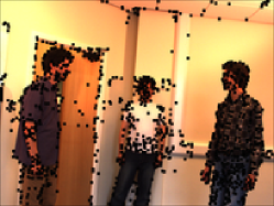
(a)

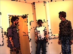
(b)

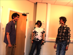
(c)

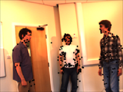
(d)

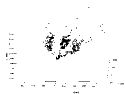
(e)

Figure 7: Interest points as detected in the left (a) and right (b) images. Dynamic interest points detected in the left (c) and the right (d) images. (e) HM3D visual observations, $\{\mbox{\boldmath$v$}_{m}\}_{m=1}^{M}$. Most of the background (hence static) points are filtered out from (a) to (c) and from (b) to (d). It is worth noticing that the reconstructed HM3D features suffer from reconstruction errors.

(a)

(b)

Figure 8: Observation densities in the auditory space $\mathbb{A}$: (a) of the projected HM3D features, $\{\tilde{\mbox{\boldmath$v$}}_{m}\}_{m=1}^{M}$, and (b) of the ITD features, $\{\mbox{\boldmath$a$}_{k}\}_{k=1}^{K}$. In this particular example, we observe three moving objects (corresponding to the three people in the images). In addition, two of them are emitting sound (left and middle) and one is silent (right). We remark that auditory as well as visual observations are contaminated by noise (enlarging the Gaussian variances) and by outliers (uniformly distributed in the auditory feature space).

To quantitatively evaluate the localization results, we compute a distance matrix between the detected clusters and the ground-truth clusters. The cluster-to-cluster distance corresponds to the Euclidean distance between cluster means. Let $\mathbf{D}$ be the distance matrix, then entry $D_{ij}=\|\mu_{i}-\hat{\mu}_{j}\|$ is the distance from the $i^{\textrm{th}}$ ground-truth cluster to the $j^{\textrm{th}}$ detected cluster. Next, we associate at most one ground-truth cluster to each detected cluster. The assignment procedure is as follows. For each detected cluster we compute its ground-truth nearest cluster. If it is not closer than a threshold $\tau_{\textrm{loc}}$ we mark it as a false positive, otherwise we assign the detected cluster to the ground-truth cluster. Then, for each ground-truth cluster we determine how many detected clusters are assigned to it. If there is none, we mark the ground-truth cluster as false negative. Finally, for each of the remaining ground-truth clusters, we select the closest (true positive) detected cluster among the ones assigned to the ground-truth cluster and we mark the remaining ones as false positives. We can evaluate the localization error and the auditory state for those clusters that have been correctly detected . The localization error corresponds to the Euclidean distance between the means. Notice that by choosing $\tau_{\textrm{loc}}$, we fix the maximum localization error allowed. The auditory state is counted as false positive if detected audible when silent, false positive if detected silent when audible and true positive otherwise. $\tau_{\textrm{loc}}$ was set to $0.35\,\textrm{m}$ in all the experiments.

7.1 Results on Synthetic Data

Four synthetic sequences containing one to three AV objects were generated. These objects can move and they are not necessarily visible/audible along the entire sequence. Table 1 shows the visual evaluation of the method when tested with synthetic sequences. The sequence code name describes the dynamic character of the sequence (Sta means static and Dyn means dynamic) and the varying number of AV objects in the scene (Con means constant number of AV objects and Var means varying number of AV objects). The columns show different evaluation quantities: FP (false positives), i.e., AV objects found that do not really exist, FN (false negatives), i.e., present AV objects that were not found, TP (true positives) and ALE (average localization error). Recall that we can compute the localization error just for the true positives. First, we observe that the right detection rate is always above 65%, increasing to 96% in the case where there are 3 visible static clusters. We also observe that the fact that the number of AV objects in the scene varies does not impact the localization error. The effect on the localization error is due, hence, to the dynamic character of the scene; if the AV objects move or not. The third observation is that both the dynamic character of the scene and the varying number of clusters have a lot of impact on the detection rate.

Table 1: Visual evaluation of results obtained with synthetic sequences. Sta/Dyn states for static or dynamic scene; the AV objects move or do not move. Var/Con states for varying or constant number of AV objects. FP stands for false positives, FN for false negatives, TP for true positives and ALE for average localization error (expressed in meters).

Seq.	FP	FN	TP	ALE [m]
StaCon	12	16 (3.9%)	392 (96.1%)	0.03
DynCon	43	139 (34.1%)	269 (65.9%)	0.10
StaVar	46	69 (30.1%)	160 (69.9%)	0.03
DynVar	40	82 (35.9%)	147 (64.1%)	0.11

Table 2: Audio evaluation of the results obtained with synthetic sequences. Sta/Dyn states for static or dynamic scene; the AV objects move or do not move. Var/Con states for varying or constant number of AV objects.

Seq.	FP	FN	TP
StaCon	161	33 (13.4%)	214 (86.6%)
DynCon	144	56 (21.2%)	208 (78.8%)
StaVar	53	33 (18.8%)	143 (81.2%)
DynVar	56	34 (19.7%)	139 (80.3%)

Table 2 shows the auditory evaluation of the method when tested with synthetic sequences. The remarkable achievement is the high number of right detections, around 80%, in all cases. This means that neither the dynamic character of the scene nor the fact that the number of AV objects varies have an impact on sound detection. It is also true that the number of false positives is large in all the cases.

7.2 Results on Real Data

The Motion-Guided Robot Hearing method was tested on the CTMS3 sequence of the CAVA data set [Arnaud 08]. The CAVA (computational audio-visual analysis) data set was specifically recorded to test various real-world audio-visual scenarios. The CTMS3 sequence consists on three people freely moving in a room and taking speaking turns. Two of them count in English (one, two, three, …) while the third one counts in Chinese. The recorded signals, both auditory and visual, enclose the difficulties found in natural situations. Hence, this is a very challenging sequence: People come in and out the visual field of the two cameras, hide each other, etc. Aside from the speech sounds, there are acoustic reverberations and non-speech sounds such as those emitted by foot steps and clothe chafing. Occasionally, two people speak simultaneously.

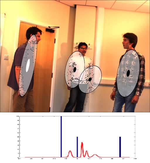
(a)

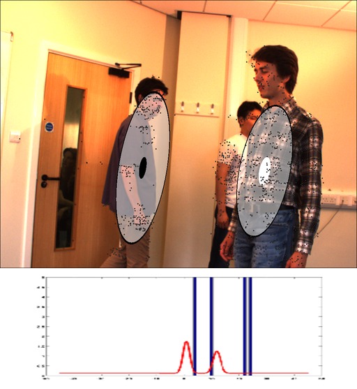
(b)

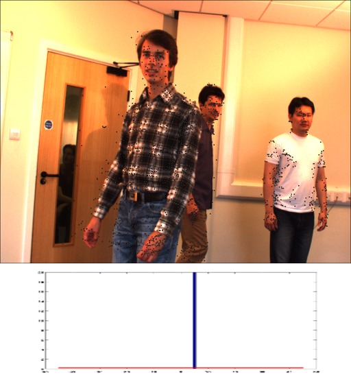
(c)

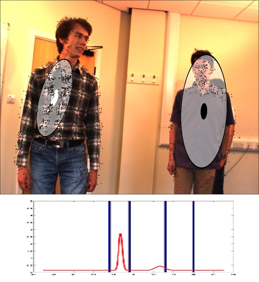
(d)

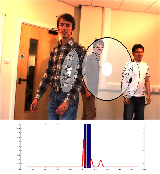
(e)

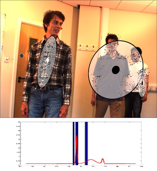
(f)

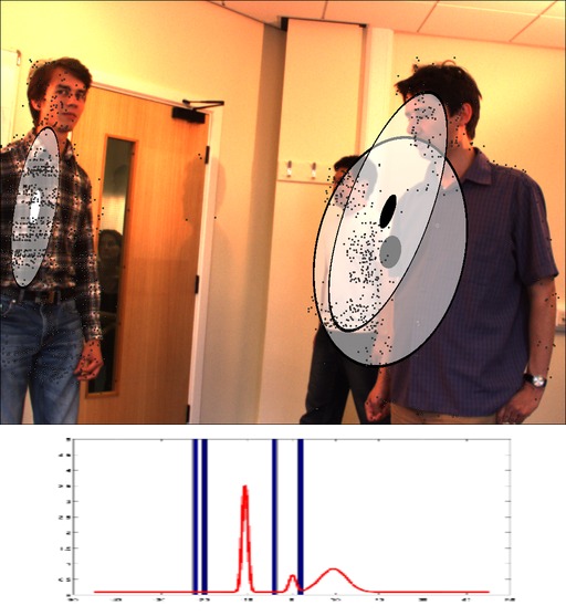
(g)

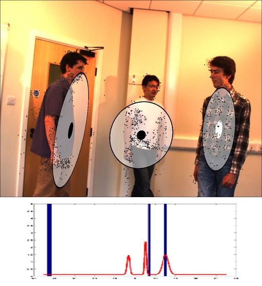
(h)

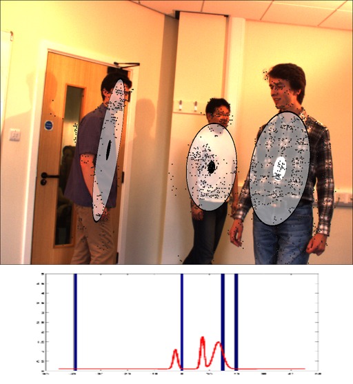
(i)

Figure 9: Results obtained with the CTMS3 sequence from the CAVA data set. The ellipses correspond to the 3D covariance matrices projected onto the image. The circle at each ellipse center illustrates the auditory activity: speaker emitting a sound (white) or being silent (black) during each time interval. The plot associated with each image shows the auditory observations as well as the fitted 1D mixture model.

Figure 9 shows the results obtained with nine time intervals chosen to show both successes and failures of our method and to allow to qualitatively evaluate it. Figure 9a shows one extreme case, in which the distribution of the HM3D observations associated to the person with the white T-shirt is clearly not Gaussian. Figure 9b shows a failure of the ridgeline method, used to merge Gaussian components, where two different clusters are associated into one. Figure 9c is an example with too few observations. Indeed, the BIC points as optimal the model with no AV objects, thus considering all the observations to be outliers. Figure 9d clearly shows that our approach cannot deal with occluded objects, because of the instantaneous processing of robocentric data, the person occluded will never be detected. Figures 9e, 9f and 9g are examples of success. The three speakers are localised and their auditory status correctly guesses. However, the localisation accuracy is not good in these cases, because one or more covariance matrices are not correctly estimated. The grouping of AV observations is, then, not well conducted. Finally, Figures 9h and 9i show two case in which the Motion-Guided Robot Hearing algorithms works perfectly, three people are detected and their speaking activity is correctly assessed from the ITD observations. In average, the method correctly detected 187 out of 213 objects (87.8%) and correctly detected the speaking state in 88 cases out of 147 (59.9%).

7.3 Results on NAO

To validate the Face-Guided Robot Hearing method using NAO, we performed a set of experiments with five different scenarios. The scenarios were recorded in a room around $5\times 5$ meters with just a sofa and 3 chairs where NAO and the other persons sat respectively. We designed five scenarios to test the algorithm in different conditions in order to identify its limitations. Each scenario is repeated several times and consists on people counting from one up to sixteen.

In scenario S1, only one person is in the room sitting in front of the robot and counting. In the rest of the scenarios (S2-S5) three persons are in the room. People are not always in the field of view (FoV) of the cameras and sometimes they move. In scenario S2 three persons are sitting and counting alternatively one after the other. The configuration of scenario S3 is similar to the one of S2, but one person is standing instead of sitting. These two scenarios are useful to determine the precision of the ITDs and experimentally see if the difference of height (elevation) affects the quality of the extracted ITDs. The scenario S4 is different from S2 and S3 because one of the actors is outside the FoV. This scenario is used to test if people speaking outside the FoV affect the performance of the algorithm. In the last scenario (S5) the three people are in the FoV, but they count and speak independently of the other actors. Furthermore, one of them is moving while speaking. With S5, we aim to test the robustness of the method to dynamic scenes.

In Figure 10 we show several snapshots of our visualization tool. These frames are selected from the different scenarios aiming to show both the successes and the failures of the implemented system. Figure 10a shows an example of perfect alignment between the ITDs and the mapped face, leading to a high speaking probability. A similar situation is presented in Figure 10b, in which among the three people, only one speaks. A failure of the ITD extractor is shown in Figure 10c, where the actor in the left is speaking, but no ITDs are extracted. In Figure 10d we can see how the face detector does not work correctly: two faces are missing, one because of the great distance between the robot and the speaker, and the other because it is partially out of the field of view. Figure 10e shows a snapshot of an AV-fusion failure, in which the extracted ITDs are not significant enough to set a high speaking probability. The Figure 10f, Figure 10g and Figure 10h show the effect of reverberations. While in Figure 10h we see that the reverberations lead to the wrong conclusion that the actor on the right is speaking, we also see that the statistical framework is able to handle reverberations (Figure 10f and Figure 10g), hence demonstrating the robustness of the proposed approach.

Table 3 shows the results obtained on scenarios (that were manually annotated). First of all we notice the small amount of false negatives: the system misses very few speakers. A part from the first scenario (easy conditions), we observe some false positives. These false positives are due to reverberations. Indeed, we notice how the percentage of FP is severe in S5. This is due to the fact that high reverberant sounds (like hand claps) are also present in the audio stream of this scenario. We believe that an ITD extraction method more robust to reverberations will lead to more reliable ITD values, which in turn will lead to a better active speaker detector. It is also worth to notice that actors in different elevations and non-visible actors do not affect the performance of the proposed system, since the results obtained in scenarios S2 to S4 are comparable.

	FP	FN	TP
S1	13	23 (13.4%)	149 (86.6%)
S2	22	31 (14.9%)	176 (85.1%)
S3	19	20 (11.3%)	157 (88.7%)
S4	37	12 (6.7%)	166 (93.3%)
S5	53	32 (19.0%)	136 (81.0%)

Table 3: Quantitative evaluation of the proposed approach for the five scenarios. The columns represent, in order: the amount of correct detections (CD), the amount of false positives (FP), the amount of false negatives (FN) and the total number of counts (Total).

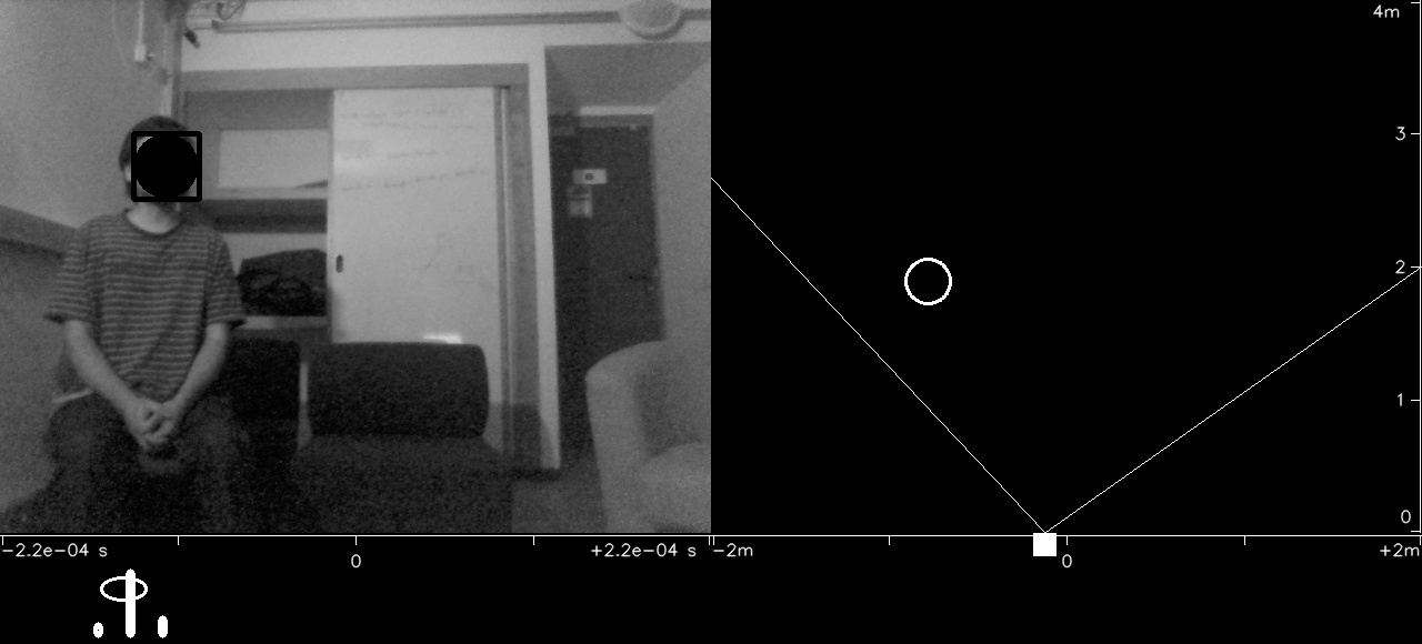
(a) S1

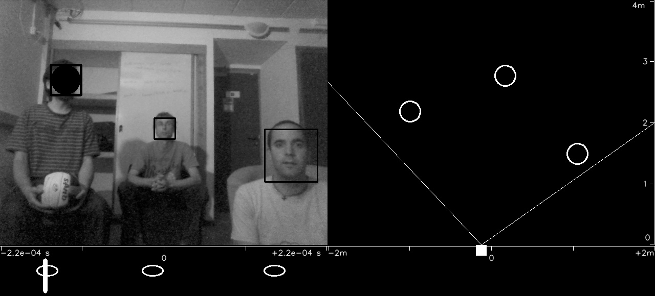
(b) S2

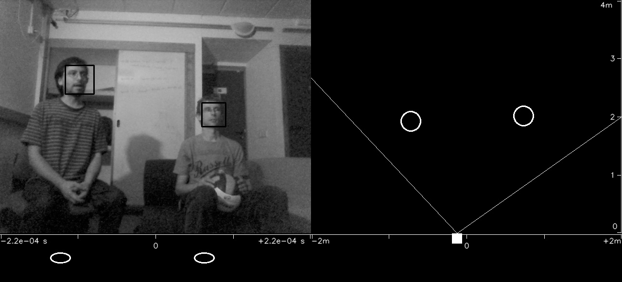
(c) S4

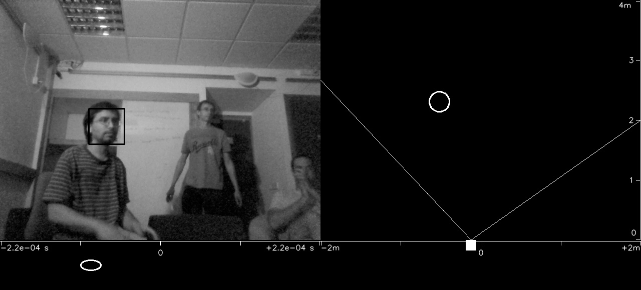
(d) S5

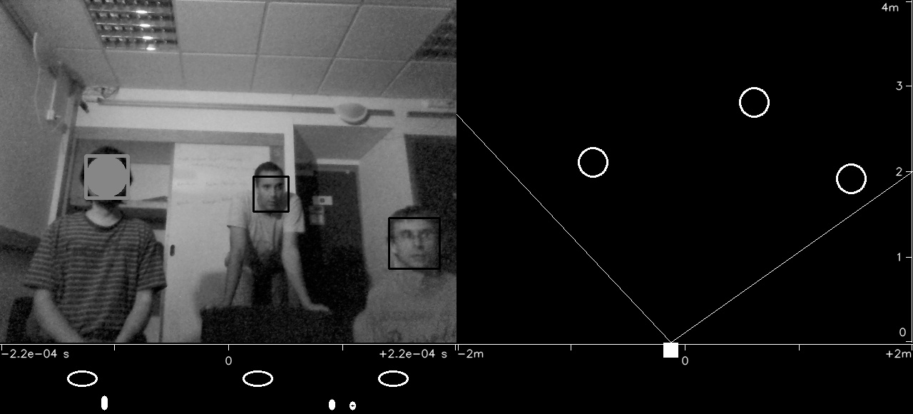
(e) S5

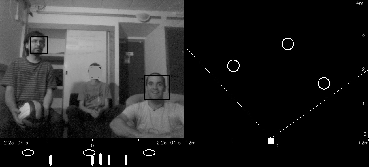
(f) S2

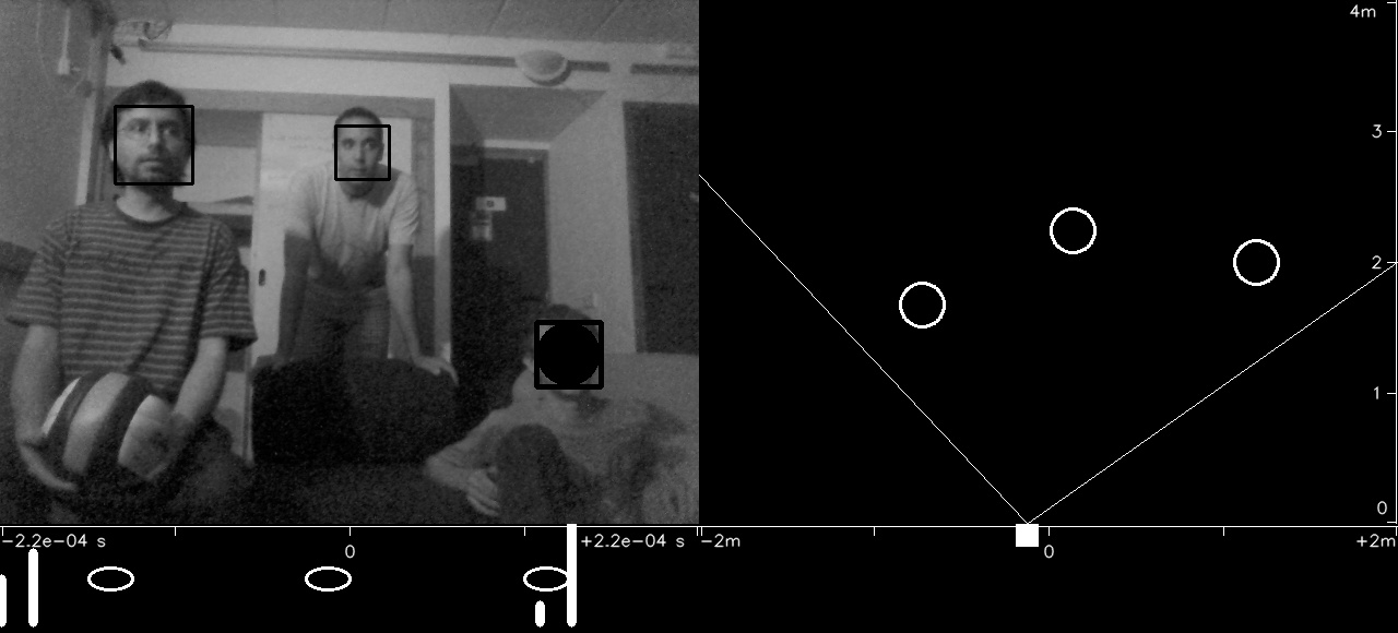
(g) S3

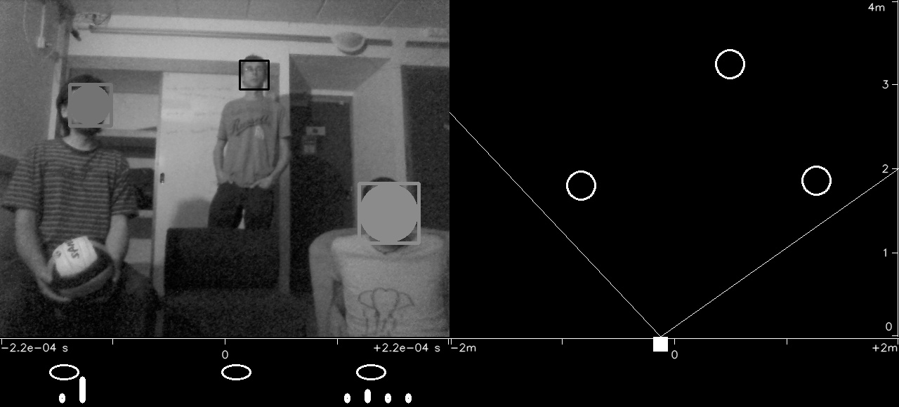
(h) S3

Figure 10: Snapshots of the visualization tool. Frames selected among the five scenarios to show the method’s strengths and weaknesses. The faces’ bounding box are shown superposed to the original image (top-left). The bird-view of the scene is shown in the top-right part of each subimage. The histogram of ITD values as well as the projected faces are shown in the bottom-left. See Section 6.3 for how to interpret the images above.

8 Conclusions and Future Work

This paper introduces a multimodal hybrid probabilistic/deterministic framework for simultaneous detection and localization of speakers. On one hand, the deterministic component takes advantage of the geometric and physical properties associated with the visual and auditory sensors: the audio-visual mapping $(\overline{\cal A}\circ{\cal V})$ allows us to transform the visual features from the 3D space to an 1D auditory space. On the other hand, the probabilistic model deals with the observation-to-speaker assignments, the noise and the outliers. We propose a new multimodal clustering algorithm based on a 1D Gaussian mixture model, an initialization procedure, and a model selection procedure based on the BIC score. The method is validated on a humanoid robot and interfaced through the RSB middleware leading to a platform-independent implementation.

The main novelty of the approach is the visual guidance. Indeed, we derived to EM-based procedures for Motion-Guided and Face-Guided robot hearing. Both algorithms provide the number of speakers, localize them and ascertain their speaking status. In other words, we show how one of the two modalities can be used to supervise the clustering process. This is possible thanks to the audio-visual calibration procedure that provides an accurate projection mapping $(\overline{\cal A}\circ{\cal V})$. The calibration is specifically designed for robotic usage since it requires very few data, it is long-lasting and environment-independent.

The presented method solves several open methodological issues: (i) it fuses and clusters visual and auditory observations that lie in physically different spaces with different dimensionality, (ii) it models and estimates the object-to-observation assignments that are not known, (iii) it handles noise and outliers mixed with both visual and auditory observations whose statistical properties change across modalities, (iv) it weights the relative importance of the two types of data, (v) it estimates the number of AV objects that are effectively present in the scene during a short time interval and (vi) it gauges the position and speaking state of the potential speakers.

One prominent feature of our algorithm is its robustness. It can deal with various kinds of perturbations, such as the noise and outlier encountered in unrestricted physical spaces. We illustrated the effectiveness and robustness of our algorithm using challenging audio-visual sequences from a publicly available data set as well as using the humanoid robot NAO in regular indoor environments. We demonstrated good performance on different scenarios involving several actors, moving actors and non-visible actors. Interfaced by means of the RSB middleware, the Face-Guided Robot Hearing method processes the audio-visual data flow from two microphones mounted inside the head of a companion robot with noisy fans and two cameras at a rate of 17 Hz.

There are several possible ways to improve and to extend our method. Our current implementation relies more on the visual data than on the auditory data, although there are many situations where the auditory data are more reliable. The problem of how to weight the relative importance of the two modalities is under investigation. Our algorithm can also accommodate other types of visual cues, such as 2D or 3D optical flow, body detectors, etc., or auditory cues, such as Interaural Level Differences. In this paper we used one pair of microphones, but the method can be easily extended to several microphone pairs. Each microphone pair yields one ITD space and combining these 1D spaces would provide a much more robust algorithm. Finally, another interesting direction of research is to design a dynamic model that would allow to initialize the parameters in one time interval based on the information extracted in several previous time intervals. Such a model would necessarily involve dynamic model selection, and would certainly help to guess the right number of AV objects, particularly in situations where a cluster is occluded but still in the visual scene, or a speaker is highly interfered by another speaker/sound source. Moreover, this future dynamic model selection should be extended to provide for audio-visual tracking capabilities, since they enhance the temporal coherence of the perceived audio-visual scene.

References

- [Alameda-Pineda 11] X. Alameda-Pineda, V. Khalidov, R. Horaud & F. Forbes. Finding audio-visual events in informal social gatherings. In Proceedings of the ACM/IEEE International Conference on Multimodal Interaction, 2011.
- [Anastasio 00] T. J. Anastasio, P. E. Patton & K. E. Belkacem-Boussaid. Using Bayes’ Rule to Model Multisensory Enhancement in the Superior Colliculus. Neural Computation, vol. 12, no. 5, pages 1165–1187, 2000.
- [Arnaud 08] E. Arnaud, H. Christensen, Y.-C. Lu, J. Barker, V. Khalidov, M. Hansard, B. Holveck, H. Mathieu, R. Narasimha, E. Taillant, F. Forbes & R. P. Horaud. The CAVA corpus: synchronised stereoscopic and binaural datasets with head movements. In Proceedings of the ACM/IEEE International Conference on Multimodal Interfaces, 2008. http://perception.inrialpes.fr/CAVA_Dataset/.
- [Barker 09] J. Barker & X. Shao. Energetic and Informational Masking Effects in an Audiovisual Speech Recognition System. Audio, Speech, and Language Processing, IEEE Transactions on, vol. 17, no. 3, pages 446–458, 2009.
- [Barzelay 07] Z. Barzelay & Y. Schechner. Harmony in Motion. In CVPR, 2007.
- [Besson 08a] P. Besson & M. Kunt. Hypothesis testing for evaluating a multimodal pattern recognition framework applied to speaker detection. Journal of NeuroEngineering and Rehabilitation, vol. 5, no. 1, page 11, 2008.
- [Besson 08b] P. Besson, V. Popovici, J. Vesin, J. Thiran & M. Kunt. Extraction of Audio Features Specific to Speech Production for Multimodal Speaker Detection. Multimedia, IEEE Transactions on, vol. 10, no. 1, pages 63 –73, jan. 2008.
- [Bishop 06] C. M. Bishop. Pattern recognition and machine learning (information science and statistics). Springer-Verlag New York, Inc., Secaucus, NJ, USA, 2006.
- [Bouguet 08] J.-Y. Bouguet. Camera Calibration Toolbox for Matlab. http://www.vision.caltech.edu/bouguetj/calib\_doc/, 2008.
- [Butz 05] T. Butz & J.-P. Thiran. From error probability to information theoretic (multi-modal) signal processing. Signal Process., vol. 85, no. 5, pages 875–902, May 2005.
- [Calvert 04] G. Calvert, C. Spence & B. E. Stein. The handbook of multisensory processes. MIT Press, 2004.
- [Christensen 07] H. Christensen, N. Ma, S. Wrigley & J. Barker. Integrating Pitch and Localisation Cues at a Speech Fragment Level. In Proc. of Interspeech, pages 2769–2772, 2007.
- [Davies 79] D. Davies & D. Bouldin. A Cluster Separation Measure. Pattern Analysis and Machine Intelligence, IEEE Transactions on, vol. PAMI-1, no. 2, pages 224–227, January 1979.
- [Dempster 77] A. Dempster, N. Laird & D. Rubin. Maximum likelihood from incomplete data via the EM algorithm. Journal of the Royal Statistical Society. Series B (Methodological), vol. 39, no. 1, pages 1–38, 1977.
- [Gatica-Perez 07] D. Gatica-Perez, G. Lathoud, J.-M. Odobez & I. McCowan. Audiovisual probabilistic tracking of multiple speakers in meetings. IEEE Transactions on Audio, Speech, and Language Processing, vol. 15, no. 2, pages 601–616, 2007.
- [Ghazanfar 06] A. A. Ghazanfar & C. E. Schroeder. Is neocortex essentially multisensory? Transactions on Cognitive Neuroscience, vol. 10, page 278–285, 2006.
- [Gurban 06] M. Gurban. Multimodal speaker localization in a probabilistic framework. In In Proc. of EUSIPCO, 2006.
- [Hansard 08] M. Hansard & R. P. Horaud. Cyclopean Geometry of Binocular Vision. Journal of the Optical Society of America, vol. 25, no. 9, page 2357–2369, September 2008.
- [Harris 88] C. Harris & M. Stephens. A Combined Corner and Edge Detector. In Proc. of Fourth Alvey Vision Conference, pages 147–151, 1988.
- [Hartley 04] R. I. Hartley & A. Zisserman. Multiple view geometry in computer vision. Cambridge University Press, ISBN: 0521540518, second edition, 2004.
- [Haykin 05] S. Haykin & Z. Chen. The Cocktail Party Problem. Journal on Neural Compututation, vol. 17, pages 1875–1902, September 2005.
- [Hennig 10] C. Hennig. Methods for merging Gaussian mixture components. Advances in Data Analysis and Classification, vol. 4, pages 3–34, 2010. 10.1007/s11634-010-0058-3.
- [Hospedales 08] T. Hospedales & S. Vijayakumar. Structure Inference for Bayesian Multisensory Scene Understanding. IEEE Transactions on Pattern Analysis and Machine Intelligence, vol. 30, no. 12, pages 2140–2157, 2008.
- [Itohara 11] T. Itohara, T. Otsuka, T. Mizumoto, T. Ogata & H. G. Okuno. Particle-Filter Based Audio-Visual Beat-Tracking for Music Robot Ensemble with Human Guitarist. In IROS, 2011.
- [Itohara 12] T. Itohara, K. Nakadai, T. Ogata & H. G. Okuno. Improvement of Audio-Visual Score Following in Robot Ensemble with Human Guitarist. In IEEE-RAS International Conference on Humanoid Robots, 2012.
- [Keribin 00] C. Keribin. Consistent Estimation of the Order of Mixture Models. Sankhya Series A, vol. 62, no. 1, pages 49–66, 2000.
- [Khalidov 08] V. Khalidov, F. Forbes, M. Hansard, E. Arnaud & R. Horaud. Detection and Localization of 3D Audio-Visual Objects Using Unsupervised Clustering. In ICMI ’08, pages 217–224, New York, NY, USA, 2008. ACM.
- [Khalidov 11] V. Khalidov, F. Forbes & R. Horaud. Conjugate Mixture Models for Clustering Multimodal Data. Journal on Neural Computation, vol. 23, no. 2, pages 517–557, February 2011.
- [Kidron 05] E. Kidron, Y. Y. Schechner & M. Elad. Pixels that Sound. In Proceedings of the 2005 IEEE Computer Society Conference on Computer Vision and Pattern Recognition (CVPR’05) - Volume 1 - Volume 01, CVPR ’05, pages 88–95, Washington, DC, USA, 2005. IEEE Computer Society.
- [Kidron 07] E. Kidron, Y. Schechner & M. Elad. Cross-Modal Localization via Sparsity. Trans. Sig. Proc., vol. 55, no. 4, pages 1390–1404, April 2007.
- [Kim 07] H. Kim, J. suk Choi & M. Kim. Human-Robot Interaction in Real Environments by Audio-Visual Integration. International Journal of Control, Automation and Systems, vol. 5, no. 1, pages 61–69, 2007.
- [King 09] A. J. King. Visual influences on auditory spatial learning. Philosophical Transactions of the Royal Society B: Biological Sciences, vol. 364, no. 1515, pages 331–339, 2009.
- [Liu 08] M. Liu, Y. Fu, & T. S. Huang. An Audio-Visual Fusion Framework with Joint Dimensionality Reduction. In Proceedings of the IEEE International Conference on Audio Speech and Signal Processing, 2008.
- [Miller 03] D. Miller & J. Browning. A mixture model and EM-based algorithm for class discovery, robust classification, and outlier rejection in mixed labeled/unlabeled data sets. IEEE Transactions on Pattern Analysis and Machine Intelligence, vol. 25, no. 11, pages 1468 – 1483, nov. 2003.
- [Nakadai 04] K. Nakadai, D. Matsuura, H. G. Okuno & H. Tsujino. Improvement of recognition of simultaneous speech signals using AV integration and scattering theory for humanoid robots. Speech Communication, pages 97–112, 2004.
- [Nakamura 11] T. Nakamura, T. Nagai & N. Iwahashi. Bag of multimodal LDA models for concept formation. In Robotics and Automation (ICRA), 2011 IEEE International Conference on, pages 6233–6238, 2011.
- [Naqvi 10] S. Naqvi, M. Yu & J. Chambers. A Multimodal Approach to Blind Source Separation of Moving Sources. Selected Topics in Signal Processing, IEEE Journal of, vol. 4, no. 5, pages 895–910, 2010.
- [Natarajan 12] P. Natarajan, S. Wu, S. N. P. Vitaladevuni, X. Zhuang, S. Tsakalidis, U. Park, R. Prasad & P. Natarajan. Multimodal feature fusion for robust event detection in web videos. In Proceedings of the IEEE International Conference on Computer Vision an Pattern Recognition, 2012.
- [Nigam 00] K. Nigam, A. McCallum, S. Thrun & T. Mitchell. Text Classification from Labeled and Unlabeled Documents using EM. Machine Learning, vol. 39, no. 2-3, pages 103–134, 2000.
- [Noulas 12] A. Noulas, G. Englebienne & B. Krose. Multimodal Speaker Diarization. Pattern Analysis and Machine Intelligence, IEEE Transactions on, vol. 34, no. 1, pages 79–93, 2012.
- [Ray 05] S. Ray & B. G. Lindsay. The topography of multivariate normal mixtures. The Annals of Statistics, vol. 33, no. 5, pages 2042–2065, 2005.
- [ROS 12] ROS. message_filters/ApproximateTime. http://www.ros.org/wiki/message_filters/ApproximateTime, 2012. accessed: 06/21/02012.
- [Sanchez-Riera 12] J. Sanchez-Riera, X. Alameda-Pineda, J. Wienke, A. Deleforge, S. Arias, J. Čech, S. Wrede & R. P. Horaud. Online Multimodal Speaker Detection for Humanoid Robots. In IEEE International Conference on Humanoid Robotics, Osaka, Japan, November 2012.
- [Schwarz 78] G. Schwarz. Estimating the dimension of a model. The Annals of Statistics, vol. 6, pages 461–464, 1978.
- [Senkowski 08] D. Senkowski, T. R. Schneider, J. J. Foxe & A. K. Engel. Crossmodal binding through neural coherence: Implications for multisensory processing. Trends in Neuroscience, vol. 31, no. 8, page 401–409, 2008.
- [Šochman 05] J. Šochman & J. Matas. WaldBoost – Learning for Time Constrained Sequential Detection. In Proceedings of the IEEE Computer Vision and Pattern Recognition, 2005.
- [Wienke 11] J. Wienke & S. Wrede. A Middleware for Collaborative Research in Experimental Robotics. In 2011 IEEE/SICE Internatinal Symposium on System Integration, Kyoto, Japan, 2011. IEEE, IEEE.