Crystalline Confinement

Abstract:

We show that exotic phases arise in generalized lattice gauge theories known as quantum link models in which classical gauge fields are replaced by quantum operators. While these quantum models with discrete variables have a finite-dimensional Hilbert space per link, the continuous gauge symmetry is still exact. An efficient cluster algorithm is used to study these exotic phases. The $(2+1)$-d system is confining at zero temperature with a spontaneously broken translation symmetry. A crystalline phase exhibits confinement via multi-stranded strings between charge-anti-charge pairs. A phase transition between two distinct confined phases is weakly first order and has an emergent spontaneously broken approximate $SO(2)$ global symmetry. The low-energy physics is described by a $(2+1)$-d $\mathbb{R}P(1)$ effective field theory, perturbed by a dangerously irrelevant $SO(2)$ breaking operator, which prevents the interpretation of the emergent pseudo-Goldstone boson as a dual photon. This model is an ideal candidate to be implemented in quantum simulators to study phenomena that are not accessible using Monte Carlo simulations such as the real-time evolution of the confining string and the real-time dynamics of the pseudo-Goldstone boson.

1 Introduction

Lattice gauge theories have made fundamental contributions to our understanding of strongly correlated systems. In particle physics, the $SU(3)$ lattice gauge theory with Wilson and staggered fermions, and more recently with twisted mass, overlap, and domain wall fermions, are extensively used to investigate the properties of Quantum Chromodynamics (QCD). In condensed matter physics, the study of deconfined quantum critical points, as well as of spin liquids, employ $U(1)$ lattice gauge theories. The toric code studied in the condensed matter and the quantum information community is a $\mathbf{Z}(2)$ lattice gauge theory.

Non-perturbative studies of lattice gauge theories almost exclusively use Monte Carlo simulations in Euclidean space-time. The conventional formulation is due to Wilson, using parallel transporter matrices on the links of the lattice and matter fields on the sites. This method has been very successful in several respects, such as in the ab-initio calculation of the hadron spectrum as well as the nature of the finite temperature transition of strongly interacting matter in QCD. However, there are certain important problems where this method fails. Two of the most important examples are the physics at non-zero baryon density and the real-time evolution of quantum systems. In these cases, the weights to be sampled with Monte Carlo become negative, or even complex. The importance sampling fails, thus leading to a sign problem.

The rapid development of the field of ultra-cold atoms in optical lattices suggests a remarkable way out of this problem. The basic idea that the use of quantum variables could speed up the simulation tremendously was conceived early on [1]. Special purpose quantum computers, known as quantum simulators [2], are used as digital [3] or analog devices [4] to simulate strongly coupled quantum systems. Recently, the use of quantum simulators to study the real-time evolution in gauge theories and their phase structure in the context of particle physics has been proposed [5, 6, 7, 8, 9, 10, 11, 12, 13]. The idea behind the quantum simulator constructions is that the quantum mechanical nature of quarks and gluons can be embodied by ultra-cold atoms in optical lattices. The interactions between the atoms can be tuned, so that they follow a properly designed Hamiltonian. The quantum degrees of freedom evolve according to this Hamiltonian and the sign problem does not arise. A number of important models, such as the Bose-Hubbard model and the toric code, have already been quantum simulated using similar methods [14, 15].

In this context, the use of alternative formulations of gauge theories is highly desirable, the principal motivation being the identification of models with a finite-dimensional Hilbert space at each link or site which can be realized with a few quantum states of a cold atom system. The Hamiltonian formulation of Wilson’s lattice gauge theory has an infinite-dimensional Hilbert space at each link due to the use of continuously varying fields. Quantum link models (QLMs) provide such an alternative formulation of gauge theories [16, 17, 18, 19, 20] which realize continuous gauge symmetry with generalized quantum spins associated with the links of a lattice. They constitute an extension of the Wilsonian formulation of lattice gauge theories. Indeed, in certain limiting cases, Wilson’s lattice gauge theories can be obtained from quantum link models [21]. Because they use discrete degrees of freedom, the Hilbert space of quantum link models at every link is finite-dimensional in a completely gauge invariant way. This enables a direct connection with ultra-cold atoms in optical lattices, where the generalized quantum spins can be represented by these atoms. Therefore, quantum link models are ideal candidates to be implemented in cold atom systems.

The regularization of a $d$-dimensional quantum field theory formulated with discrete quantum variables in $(d+1)$-dimensions (instead of using classical fields) is known as the D-theory formulation [20]. The classical fields in the $d$-dimensional quantum field theory emerge as low-energy effective degrees of freedom of the discrete variables when the $(d+1)$-dimensional theory has a massless Coulomb phase. When the extra Euclidean dimension is made small in units of the correlation length, a $d$-dimensional theory emerges by dimensional reduction. For example, in the D-theory formulation of QCD, the confining gluon field emerges by dimensional reduction from a deconfined Coulomb phase of a $(4+1)$-d $SU(3)$ quantum link model. Chiral quarks can be included naturally as domain wall fermions located at the two 4-d sides of a $(4+1)$-d slab [19].

Quantum link models also provide a platform for developing efficient simulation algorithms. As they are formulated with discrete variables, they are natural candidates to develop cluster algorithms. The phase diagrams of these models are obviously interesting to study. Since they are generalized lattice gauge theories, new phases arise, which have not been observed in Wilson-type lattice gauge theories. Also, once quantum simulators are being built, they need to be validated against controlled classical computations. By developing methods to simulate quantum link models, static quantities can be calculated to benchmark the quantum simulators. Finally, methods developed for simulating link models might be applicable to solve some of the sign problems in traditional Wilson-type theories at non-zero density.

In this article, we report on a study of the $(2+1)$-dimensional $U(1)$ quantum link model and show that, despite its structural simplicity, it has a very rich phase diagram [22]. This model has exotic confining phases where the confining string joining a static charge-anti-charge pair splits into distinct fractionalized flux $\frac{1}{2}$ strands. There are two such phases, each characterized by a distinct pattern of discrete symmetry breaking, separated by a weak first-order transition. Around the phase transition point, there is a spontaneously broken approximate global $SO(2)$ symmetry arising dynamically. The resulting pseudo-Goldstone boson can be described via an effective field theory. When realized with quantum simulators, this model would be able to demonstrate the power of gauge theory simulators by quantum simulating the dynamics of the confining string and the pseudo-Goldstone boson.

2 The $(2+1)$-d Quantum Link Model

In the Wilson formulation of $U(1)$ lattice gauge theory, the Hamiltonian takes the form

$$H=\frac{g^{2}}{2}\sum_{x,i}e^{2}_{x,i}-\frac{1}{2g^{2}}\sum_{\square}(u_{\square}+u_{\square}^{\dagger}),$$ (1)

where the second sum is over all plaquettes and the plaquette variables are $u_{\square}=u_{x,i}u_{x+\hat{i},j}u_{x+\hat{j},i}^{\dagger}u_{x,j}^{\dagger}$, $u_{x,i}=\exp(i\varphi_{x,i})\in U(1)$. In this formulation they are operators acting in an infinite-dimensional Hilbert space for each link. The electric field operator $e_{x,i}$ describes the kinematics of $u_{x,i}$,

$$e_{x,i}=-i\partial_{\varphi_{x,i}},\qquad[e_{x,i},u_{y,j}]=u_{x,i}\delta_{xy}\delta_{ij},\qquad[e_{x,i},u_{y,j}^{\dagger}]=-u_{x,i}^{\dagger}\delta_{xy}\delta_{ij},\qquad[u_{x,i},u_{y,j}^{\dagger}]=0.$$ (2)

The Hamiltonian is invariant under gauge transformations since it commutes with their generators $G_{x}=\sum_{i}(e_{x,i}-e_{x-\hat{i},i})$. A general gauge transformation takes the form $u_{x,i}^{\prime}=e^{i\alpha_{x}}u_{x,i}e^{-i\alpha_{x+\hat{i}}}$.

The $(2+1)$-d $U(1)$ quantum link model is formulated in a similar way. Its Hamiltonian can be written as

$$H=\frac{g^{2}}{2}\sum_{x,i}E^{2}_{x,i}-J\sum_{\square}\left[U_{\square}+U_{\square}^{\dagger}-\lambda\left(U_{\square}+U_{\square}^{\dagger}\right)^{2}\right]$$ (3)

where the sum is over all plaquettes and the plaquette variables are defined in terms of quantum link operators, $U_{\square}:=U_{x,i}U_{x+\hat{i},j}U_{x+\hat{j},i}^{\dagger}U_{x,j}^{\dagger}$. In contrast to Wilson’s lattice gauge theory, the operators in the $U(1)$ QLM are given by a finite-dimensional representation of the embedding algebra $SU(2)$, thus leading to a finite-dimensional Hilbert space per link [18]. The quantum link variables are quantum spin raising operators $U_{x,i}=S_{x,i}^{1}+iS_{x,i}^{2}=S^{+}_{x,i}$ for the electric fluxes $E_{x,i}=S^{3}_{x,i}$, while the operators $U_{x,i}^{\dagger}$ are flux lowering operators $S_{x,i}^{-}$. The operators $U_{x,i}$, $U_{x,i}^{\dagger}$ and $E_{x,i}$ obey the same commutation relations as their counterparts in Wilson’s lattice gauge theory, except that the quantum link operators do not commute with their adjoint, i.e. $[U_{x,i},U_{x,i}^{\dagger}]=2\,E_{x,i}$. The Hamiltonian in (3) is again gauge invariant as it commutes with the generators of infinitesimal $U(1)$ gauge transformations,

$$G_{x}=\sum_{i}\left(E_{x,i}-E_{x-\hat{i},i}\right).$$ (4)

The link operators transform as $U_{x,i}^{\prime}=e^{i\alpha_{x}}U_{x,i}e^{-i\alpha_{x+\hat{i}}}$ under gauge transformations. Physical states $|\psi\rangle$ again have to be gauge invariant, i.e. they obey the Gauss law $G_{x}|\psi\rangle=Q_{x}|\psi\rangle$, where $Q_{x}$ is zero unless one places a static charge at the point $x$.

In this work we consider the simplest possible representation for the quantum links, namely the spin $\frac{1}{2}$ representation. This leads to a 2-dimensional Hilbert space per link, thereby ensuring the feasibility of exact diagonalization studies, as will be explained below. The $E_{x,i}^{2}$ term then becomes a trivial additive constant and is therefore omitted in the following. The second term in the Hamiltonian (3) flips loops of electric fluxes flowing around elementary plaquettes and annihilates non-flippable plaquettes as depicted in Fig. 1. In the spin $\frac{1}{2}$ representation, the third term, proportional to $\lambda$, is known as the Rokhsar-Kivelson (RK) term which counts flippable plaquettes. This can be seen by noting that $U_{\square}^{2}=\left(U_{\square}^{\dagger}\right)^{2}=0$, since a single spin $\frac{1}{2}$ cannot be raised more than once. The remaining terms are of the form $U_{\square}U_{\square}^{\dagger}$, i.e. they project onto the subspace of flippable plaquettes.

Figure 1: Action of the plaquette operator on flippable plaquettes (left) and non-flippable plaquettes (right). The arrows indicate the direction of the electric flux $E_{x,i}=\pm\frac{1}{2}$.

The Gauss law together with the finite-dimensional link Hilbert space reduces the number of allowed states per site from $2^{4}=16$ down to the 6 configurations shown in Fig. 2. Adding static charges reduces this number even further. Without this reduction, it would not be practical to apply exact diagonalization methods on reasonably large lattices.

Figure 2: All gauge invariant configurations of fluxes at a site $x$.

The Hamiltonian respects the usual geometric symmetries of the square lattice, e.g. it is invariant under translations by multiples of the lattice spacing $a$ and under 90 degrees rotations. For our purposes, it suffices to consider translations T only. The lattice translation invariance characterizes each energy eigenstate by its lattice momentum $p=(p_{1},p_{2})\in(-\pi,\pi]^{2}$. Additionally, the charge conjugation C symmetry is also present. It replaces $U_{x,i}$ by $U_{x,i}^{\dagger}$ and reverses all electric fluxes, i.e. $E_{x,i}$ goes to $-E_{x,i}$. The associated quantum number is the charge conjugation parity $C=\pm$. Another important global symmetry is the $U(1)$ center symmetry on periodic lattices associated with “large” gauge transformations. These are given by transformations that commute with the Hamiltonian but cannot be expressed through “small” periodic gauge transformations. On an $L_{1}\times L_{2}$ lattice they are generated by

$$E_{i}=\frac{1}{L_{i}}\sum_{x}E_{x,i}.$$ (5)

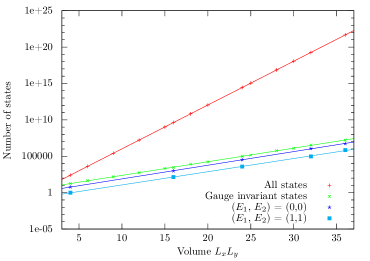
Figure 3: The total number of states in the $(2+1)$-d $U(1)$ quantum link model, both with and without imposing Gauss’ law (denoted by green ”$\times$” and red ”+” respectively). Even though the Gauss law constraint drastically decreases the number of states, the rise in the number of states is still exponential in the volume. The number of states in individual flux sectors are shown by blue stars and filled squares. Only lattices with an even extent allow the flux sectors $(0,0)$ and $(1,1)$.

3 Exact Diagonalization and Cluster Algorithm Tools

We have studied the model using both Exact Diagonalization (ED) and Quantum Monte Carlo simulations (QMC). Exact Diagonalization studies were performed on lattices with spatial extents $4\times 4$, $4\times 6$ and $6\times 6$. These systems comprise of 32, 48, and 72 quantum link spins, respectively. While the sizes may seem small, this already competes with the largest spin systems that have been subjected to ED on PC clusters. Naively, this would have implied Hilbert spaces with $2^{32}$, $2^{48}$, and $2^{72}$ states, respectively. The Gauss law constraint, however, reduces the number of states considerably, which makes the study of systems with as many as 72 spins feasible. Fig. 3 shows the number of states as a function of the volume with and without applying Gauss’ law. In these studies, the Hamiltonian was separately diagonalized in each flux winding number sector, thereby reducing the Hilbert space further than with imposing only the Gauss law constraint.

We also developed an efficient cluster algorithm to simulate the model in the dual representation. A duality transformation can be used to transform the Hamiltonian of the $(2+1)$-d quantum link model into that of a $(2+1)$-d quantum height model. This transformation is an exact rewriting of the partition function in terms of new degrees of freedom, which are quantum $\mathbb{Z}(2)$ variables located at the centers of the plaquettes. As shown in Fig. 4(a), every flux configuration can be mapped to a height configuration. A configuration of quantum height variables

$$h^{A}_{\widetilde{x}}=0,1;~{}~{}h^{B}_{\widetilde{x}}=\pm\frac{1}{2},$$ (6)

located at the dual sites $\widetilde{x}=(x_{1}+\frac{1}{2},x_{2}+\frac{1}{2})$, is associated with a flux configuration

$$E_{x,x+\hat{i}}=[h^{X}_{\widetilde{x}}-h^{X^{\prime}}_{\widetilde{x}+\hat{i}-\hat{1}-\hat{2}}]\mbox{mod}2=\pm\frac{1}{2};~{}~{}X,X^{\prime}\in\{A,B\}.$$ (7)

The cluster algorithm is then constructed by dividing the lattice into two sublattices $A$ and $B$ (illustrated by shaded and unshaded squares in Fig. 4 (a)). The $U(1)$ Gauss law constraint is implemented in the cluster building rules, which ensure that only the configurations with net zero charge at the vertices are generated. The details of the dualization procedure as well as the algorithm will be presented elsewhere [23].

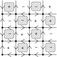
Figure 4: (a) Mapping of an electric flux configuration (shown with arrows on the links) to a height configuration (shown with $+$ and $-$ variables at the centers of the plaquettes). Every time one crosses a flux pointing right or upwards, the orientation of the plaquette variable is changed, while it remains unchanged if a left or downward pointing flux is crossed. (b) The effect of the symmetry transformations C and T on the two-component order parameter $(M_{A},M_{B})$. The former is equivalent to a reflection on the $M_{A}$ axis, while the latter is an anti-clockwise rotation by $\frac{\pi}{2}$. Performing T twice is equivalent to rotating by $\pi$, and leads back to the starting configuration, since $-(M_{A},M_{B})$ is an equivalent ”gauge” copy of $(M_{A},M_{B})$.

We define a 2-component order parameter $(M_{A},M_{B})$, associated with the even and odd sublattices $A$ and $B$, to characterize the different phases of the model. These distinguish the two different symmetry breaking patterns we encountered in our study. In terms of the height variables associated with the center of the plaquettes, they are defined as

$$M_{X}=\sum_{\widetilde{x}\in X}s^{X}_{\widetilde{x}}h^{X}_{\widetilde{x}};~{}~{}\textrm{where}~{}~{}s^{A}_{\widetilde{x}}=(-1)^{(\widetilde{x}_{1}-\widetilde{x}_{2})/2}~{}~{}\textrm{and}~{}~{}s^{B}_{\widetilde{x}}=(-1)^{(\widetilde{x}_{1}-\widetilde{x}_{2}+1)/2}.$$ (8)

Under C and T they transform as ${}^{C}M_{A}=M_{A}$, ${}^{C}M_{B}=-M_{B}$, ${}^{T}M_{A}=-M_{B}$, ${}^{T}M_{B}=M_{A}$. It should be pointed out that $\pm(M_{A},M_{B})$ represents the same physical configuration because shifting the height variables to $h^{X}_{\widetilde{x}}(t)^{\prime}=[h^{X}_{\widetilde{x}}(t)+1]\mbox{mod}2$ leaves the electric flux configuration unchanged. The various transformations are illustrated in Fig. 4(b).

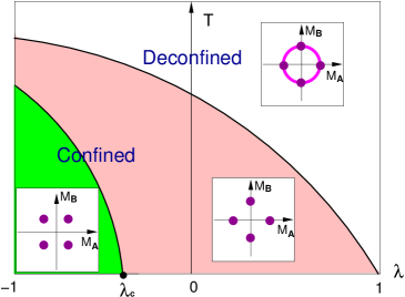
Figure 5: Schematic sketch of the $\lambda-T$ phase diagram. The insets indicate the location of the peaks in the probability distribution of the order parameter $p(M_{A},M_{B})$.

4 Phase Diagram, Order Parameters and Confining Strings

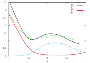
Figure 6: Energy gaps of the four lowest states on the $(6\times 6)$ lattice as a function of $\lambda$ relative to the ground state energy. The states with energies $E_{+}$ and $E_{-}$ both have non-zero momenta $(\pi,\pi)$, and are degenerate with the ground state (which has zero momentum and positive C parity) in the infinite volume limit. The state with energy $E_{-}$ has negative C parity and the state with energy $E_{+}$ has positive C parity. This implies that the spontaneous symmetry breaking pattern changes as one crosses $\lambda_{c}$. The next higher states have energies $E^{\prime}_{\pm}$ and carry momentum $(0,0)$. They have C parity $\pm$ and are used to determine the parameters of the effective theory, as described in Section 5.

The phase diagram of the model, shown in Fig. 5, was studied as a function of both $\lambda/J$ and $T/J$, where $T$ is the temperature. For convenience, we work with units in which $J=1$. At zero temperature, the model has two phases characterized by different symmetry breaking patterns for C and T. For large negative $\lambda$, both C and T are spontaneously broken. As $\lambda$ is increased beyond a critical value $\lambda_{c}$, the model undergoes a weak first order phase transition into a phase where T, but not C, is spontaneously broken.

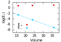
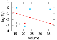
Figure 7: Finite-volume energy spectrum of the two lowest excitations above the ground state. At $\lambda~{}=~{}-1$, the state with quantum numbers $p=(\pi,\pi)$ and $C=-$ degenerates with the ground state (left). At $\lambda~{}=~{}0$, the state with quantum numbers $p=(\pi,\pi)$ and $C=+$ degenerates with the ground state (right). The ground state has positive C parity and zero momentum.

It is interesting to note that the ED results provide important insights into the phase diagram. Fig. 6 shows the energy gaps of the four lowest energy states. For $\lambda<1$, the ground state has momentum $(0,0)$ and is even under charge conjugation (i.e. $C~{}=~{}+$). For $\lambda<\lambda_{c}$, the first excited state has quantum numbers $C=-$, $p=(\pi,\pi)$. Its energy gap to the ground state, $E_{-}\sim\exp(-\sigma_{-}L_{1}L_{2})$, decreases exponentially with the volume $L_{1}L_{2}$, thus indicating the spontaneous breakdown of charge conjugation C and the translation T by one lattice spacing (in either direction). For $\lambda>\lambda_{c}$, another state $|C=+,p=(\pi,\pi)\rangle$ degenerates with the ground state in the infinite volume limit, i.e. $E_{+}\sim\exp(-\sigma_{+}L_{1}L_{2})$, indicating that C is now restored, while T remains spontaneously broken. The finite-volume scaling of the spectrum indicating these symmetry breaking patterns is shown in Fig. 7.

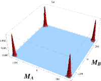
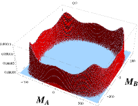
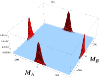
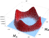
Figure 8: Distribution of the order parameter $(M_{A},M_{B})$ at $\lambda=-1$, $\lambda_{c}$, and 0 at $T=0$ (a,b,c), and at $\lambda=0$, $T>T_{c}$ (d).

These symmetry breaking patterns are clearly distinguished by the two-component order parameter $M=(M_{A},M_{B})$. The probability distribution $p(M)$ has been measured very accurately with the cluster algorithm and is shown in Fig. 8 for the different cases. At $\lambda=-1$, both sublattices are ordered, giving rise to peaks at the corners of the two-dimensional order parameter plane. At $\lambda=0$, only one sublattice is ordered, which exhibits peaks on the axes. At $\lambda=\lambda_{c}$, there is an emergent approximate global $SO(2)$ symmetry, which manifests itself by an order parameter distribution that is nearly circular. There is an emergent pseudo-Goldstone boson which can be described in terms of a low-energy effective theory. This is a remarkable phenomenon which mimics some features of deconfined quantum criticality, widely discussed in the condensed matter literature [24, 25, 26, 27, 28, 29, 30, 31, 32, 33, 34]. At $\lambda=1$ the model reaches its Rokhsar-Kivelson point. At this point electric flux condenses in the vacuum and the theory deconfines already at zero temperature.

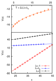
Figure 9: The potential between two static charges $\pm 2$ separated by the distance $(x,x)$ along a lattice diagonal, for $\lambda=-1,\lambda_{c}$, and 0, at $T=0$, and at $\lambda=\lambda_{c}$ for $T=2J$.

The phase diagram can also be studied as a function of temperature. Based on universality arguments, we expect that, the system undergoes a Berezinski-Kosterlitz-Thouless transition into a deconfined Coulomb phase above a temperature $T_{c}$. However, translation invariance still remains broken as evidenced by the corresponding order parameter distribution shown in Fig. 8(d). At very high temperatures, we expect all breaking of translation invariance to disappear.

Since the quantum link model is a gauge theory in $(2+1)$-dimension, we expect that it is linearly confining for $\lambda<1$ and $T=0$ [35, 36]. A standard way of demonstrating this is to place a static charge-anti-charge pair at a certain distance $r$, and then study the static potential $V(r)$ as a function of $r$. A linearly increasing potential is an unambiguous sign for confinement. The string tension $\sigma$ is given by the slope of the static potential at large distances. We have studied this by placing static charges $Q=\pm 2$ along the lattice diagonal. Our results shown in Fig. 9 exhibit linear confinement at large distances, even at the phase transition, albeit with a small string tension $\sigma_{2}=0.156(14)J/a$ (compared to $\sigma_{2}=1.97(1)J/a$ at $\lambda=-1$). Since we insert the charges explicitly in the simulation, our results for the static potential do not suffer from an exponentially small signal-to-noise ratio at larger charge-anti-charge separations.

Since translation invariance by a single lattice spacing is spontaneously broken in both the phases at $\lambda<\lambda_{c}$ and at $\lambda>\lambda_{c}$, the resulting confined phases are crystalline. The energy density $-J\langle U_{\Box}+U_{\Box}^{\dagger}\rangle$ in the presence of two charges $\pm 2$ illustrates the nature of the bulk phases. The flux string connecting the charges, shown in Fig. 10, separates into four strands of flux $\frac{1}{2}$ that repel each other. The interior of the strands consists of the phase that is stable on the other side of the transition. Near $\lambda_{c}$ the flux string undergoes topology change by wrapping one strand over the periodic boundary and materializing an additional strand at the edge of the system, whose interior then expands to become the new bulk phase (cf. Fig. 10(b)). Viewed as interfaces separating bulk phases, the strands display the universal phenomenon of complete wetting.

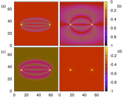
Figure 10: Energy density $-J\langle U_{\Box}+U_{\Box}^{\dagger}\rangle$ in the presence of two charges $\pm 2$ for $\lambda=-1$ (a), $\lambda=\lambda_{c}$ (b), and $\lambda=0$ (c) at $T=0$, as well as for $\lambda=0$ at $T>T_{c}$ (d).

5 Low-energy effective theory near the phase transition

The results for the histograms of the order parameter $(M_{A},M_{B})$ naturally lead to the formulation of an effective theory with an approximate $SO(2)$ symmetry in terms of a unit-vector field $\vec{e}(x)=(\cos\varphi(x),\sin\varphi(x))$ representing the direction of $(M_{A},M_{B})$. The action then takes the form

$$S[\varphi]\!=\!\int\!d^{3}x\frac{1}{c}\!\left[\frac{\rho}{2}\partial_{\mu}\varphi\partial_{\mu}\varphi\!+\!\delta\cos^{2}(2\varphi)\!+\!\varepsilon\cos^{4}(2\varphi)\right],$$ (9)

where we used $\partial_{3}=\partial_{ct}$. Here $\rho$ is the spin stiffness and $c$ is the velocity of an emergent pseudo-Goldstone boson. The $\delta$-term breaks the symmetry down to $\mathbb{Z}(4)$ and leads to a small Goldstone boson mass $Mc=2\sqrt{2|\delta|/\rho}$. The last term ensures that the string tension remains proportional to $\sqrt{\epsilon\rho}$, even at the phase transition. It is thus non-vanishing because in the effective theory the phase transition happens at $\delta_{c}+\epsilon_{c}=0$. The fact that $(M_{A},M_{B})$ is equivalent to $-(M_{A},M_{B})$ reduces the emergent symmetry from $SO(2)$ to $\mathbb{R}P(1)$. Therefore only states invariant against sign changes of $\vec{e}(x)$ belong to the physical Hilbert space.

By applying the Ginsburg-Landau-Wilson paradigm to the $\delta$- and $\epsilon$-terms, in mean field theory one obtains the phase diagram shown in Fig. 11. The two phases realized in the QLM both have four peaks in the order parameter distribution $p(M_{A},M_{B})$, and are separated by a weak first order phase transition. In addition, there is an intermediate phase with eight peaks, separated from the other phases by second order phase transitions [22].

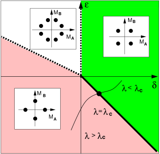
Figure 11: Phase diagram as a function of $\delta$ and $\varepsilon$. The insets indicate the location of the peaks in the distribution $p(M_{A},M_{B})$. The fat and dashed lines are first and second order phase transitions, respectively. The curved line indicates a possible path taken in the QLM when varying $\lambda$.

5.1 Comparison of the effective theory with the exact diagonalization results

Looking at the energy spectrum obtained by the exact diagonalization calculations (cf. Fig. 6), near $\lambda_{c}$ we observe an approximate finite-volume rotor spectrum $E_{m}=\frac{m^{2}c^{2}}{2\rho L_{1}L_{2}}$ for even values of $m$. In the effective theory at the phase transition we get the same spectrum. Analyzing the eigenstates for their quantum numbers, we obtain $C=+,p=(0,0)$ for the ground state $m=0$, $C=\pm,p=(\pi,\pi)$ for the next two states $m=\pm 2$ and $C=\pm,p=(0,0)$ for the $m=\pm 4$ states. All of this is consistent with the spectrum at $\lambda_{c}$ shown in Fig. 6.

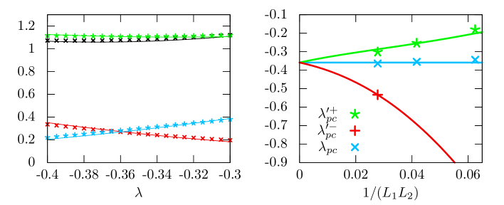
Figure 12: Global fit of the energy gaps near $\lambda_{pc}$ for $E_{\pm}$ and $E^{\prime}_{\pm}$ (left) and of the $L_{1}L_{2}$-dependence of the crossing points $\lambda_{pc}$, $\lambda^{\prime+}_{pc}$, $\lambda^{\prime-}_{pc}$ (right).

By expanding in powers of $\delta L_{1}L_{2}$ and $\epsilon L_{1}L_{2}$, we obtain predictions for the energy gaps as functions of the parameters,

$$E_{+} =\frac{2c^{2}}{\rho L_{1}L_{2}}+\frac{L_{1}L_{2}}{4}(\delta+\epsilon)+\frac{\rho L_{1}^{3}L_{2}^{3}}{256c^{2}}\left(3\delta^{2}+\frac{11}{2}\delta\epsilon+\frac{119}{48}\epsilon^{2}\right)+O(\epsilon^{3},\,\delta^{3})$$ (10)

$$E_{-} =\frac{2c^{2}}{\rho L_{1}L_{2}}-\frac{L_{1}L_{2}}{4}(\delta+\epsilon)+\frac{\rho L_{1}^{3}L_{2}^{3}}{256c^{2}}\left(3\delta^{2}+\frac{13}{2}\delta\epsilon+\frac{167}{48}\epsilon^{2}\right)+O(\epsilon^{3},\,\delta^{3})$$ (11)

$$E^{\prime}_{+} =\frac{8c^{2}}{\rho L_{1}L_{2}}+\frac{L_{1}L_{2}}{16}\epsilon+\frac{\rho L_{1}^{3}L_{2}^{3}}{128c^{2}}\left(\frac{11}{3}(\delta+\epsilon)^{2}+\frac{3}{128}\epsilon^{2}\right)+O(\epsilon^{3},\,\delta^{3})$$ (12)

$$E^{\prime}_{-} =\frac{8c^{2}}{\rho L_{1}L_{2}}-\frac{L_{1}L_{2}}{16}\epsilon+\frac{\rho L_{1}^{3}L_{2}^{3}}{128c^{2}}\left(\frac{5}{3}(\delta+\epsilon)^{2}+\frac{3}{128}\epsilon^{2}\right)+O(\epsilon^{3},\,\delta^{3})$$ (13)

$$E^{\prime\prime}_{+} =\frac{18c^{2}}{\rho L_{1}L_{2}}+\frac{\rho L_{1}^{3}L_{2}^{3}}{512c^{2}}\left(9\delta^{2}+19\delta\epsilon+\frac{409}{40}\epsilon^{2}\right)+O(\epsilon^{3},\,\delta^{3})$$ (14)

$$E^{\prime\prime}_{-} =\frac{18c^{2}}{\rho L_{1}L_{2}}+\frac{\rho L_{1}^{3}L_{2}^{3}}{512c^{2}}\left(9\delta^{2}+17\delta\epsilon+\frac{329}{40}\epsilon^{2}\right)+O(\epsilon^{3},\,\delta^{3}),$$ (15)

where the notation is the same as in Fig. 6 and $E^{\prime\prime}_{\pm}$ refer to the energy gaps of the next excited states. From the exact diagonalization results we can also extract the level crossing points $\lambda_{pc}$ (crossing of $E_{+}$ and $E_{-}$), $\lambda^{\prime+}_{pc}$ and $\lambda^{\prime-}_{pc}$ (the two crossings of $E^{\prime}_{+}$ and $E^{\prime}_{-}$). According to the effective theory, they should behave as

$$\lambda_{pc}=\lambda_{c}+\frac{A}{(L_{1}L_{2})^{2}}+O(\frac{1}{L_{1}^{3}L_{2}^{3}}),$$ (16)

$$\lambda^{\prime\pm}_{pc}=\lambda_{c}\pm\frac{1}{L_{1}L_{2}}\sqrt{-\frac{8}{c_{1}c_{2}^{2}}(c_{3}+\lambda_{c}c_{4})+\frac{16c_{4}^{2}}{c_{1}^{2}c_{2}^{4}L_{1}^{2}L_{2}^{2}}}-\frac{4c_{4}}{c_{1}c_{2}^{2}L_{1}^{2}L_{2}^{2}}+O(\frac{1}{L_{1}^{3}L_{2}^{3}}),$$ (17)

where we used the representations $\frac{\rho}{c^{2}}=c_{1}$, $\delta+\epsilon=c_{2}(\lambda-\lambda_{c})$ and $\epsilon=(c_{3}+\lambda c_{4})$. Both the energy gaps and the behavior of the different $\lambda_{pc}$ are in quantitative agreement with the exact diagonalization results. A global fit yields $\lambda_{c}=-0.359(5)$, $\delta_{c}=-\epsilon_{c}=0.01(1)\,J/a^{2}$, $\rho=0.45(3)\,J$ and $c=1.5(1)\,Ja$, where $a$ is the lattice spacing. Fig. 12 shows two exemplary comparisons of the fitted functions with the values extracted from exact diagonalization.

6 Conclusion

We have shown that even the simplest quantum link model has highly non-trivial physics involving multi-stranded confining strings and an emergent $SO(2)$ symmetry. The quantum link model studied here is very closely related to a class of models studied in condensed matter physics with connections to high-$T_{c}$ superconductivity, known as the quantum dimer models. Our methods and numerical algorithms can be straightforwardly extended to the dimer model. The corresponding investigation is in progress. Our results also encourage the application of dualization techniques to quantum Hamiltonians for other theories, and, in particular, to Hamiltonians of quantum link models in higher dimensions. The development of a quantum simulator using optical lattices to study the dynamical features of this model would be a very welcome and non-trivial step on the road to quantum simulate QCD.

References

- [1] R. P. Feynman, Int. J. Theor. Phys. 21 (1982) 467.
- [2] J. I. Cirac, P. Zoller, Phys. Rev. Lett. 74 (1995) 4091.
- [3] S. Lloyd, Science 273 (1996) 1073.
- [4] D. Jaksch, C. Bruder, J. I. Cirac, C. W. Gardiner, P. Zoller, Phys. Rev. Lett. 81 (1998) 3108.
- [5] E. Zohar, B. Reznik, Phys. Rev. Lett. 107 (2011) 275301.
- [6] G. Szirmai, E. Szirmai, A. Zamora, M. Lewenstein, Phys. Rev. A84 (2011) 011611.
- [7] Y. Liu, Y. Meurice, S.-W. Tsai, arXiv:1211.4126
- [8] E. Zohar, J. Cirac, B. Reznik, Phys. Rev. Lett. 109 (2012) 125302.
- [9] D. Banerjee, M. Dalmonte, M. Müller, E. Rico, P. Stebler, U.-J.. Wiese, P. Zoller, Phys. Rev. Lett. 109 (2012) 175302.
- [10] D. Banerjee, M. Bögli, M. Dalmonte, E. Rico, P. Stebler, U.-J.. Wiese, P. Zoller, Phys. Rev. Lett. 110 (2013) 125303.
- [11] E. Zohar, J. Cirac, B. Reznik, Phys. Rev. Lett. 110 (2013) 125304.
- [12] E. Zohar, J. Cirac, B. Reznik, Phys. Rev. A88 (2013) 023617
- [13] U.-J.. Wiese, (arXiv:1305.1602), Ann. Phys. doi: 10.1002/andp.201300104
- [14] M. Greiner, O. Mandel, T. Esslinger, T. W. Hänsch, I. Bloch, Nature 415 (2002) 39.
- [15] J. T. Barreiro, M. Müller, P. Schindler, D. Nigg, T. Monz, M. Chwalla, M. Hennrich, C. F. Roos, P. Zoller, R. Blatt, Nature 470 (2011) 486.
- [16] D. Horn, Phys. Lett. B100 (1981) 149.
- [17] P. Orland, D. Rohrlich, Nucl. Phys. B338 (1990) 647.
- [18] S. Chandrasekharan, U.-J. Wiese, Nucl. Phys. B492 (1997) 455.
- [19] R. C. Brower, S. Chandrasekharan, U.-J. Wiese, Phys. Rev. D60 (1999) 094502.
- [20] R. C. Brower, S. Chandrasekharan, S. Riederer, U.-J. Wiese, Nucl. Phys. B693 (2004) 149.
- [21] B. Schlittgen, U.-J. Wiese, Phys. Rev. D63 (2001) 085007
- [22] D. Banerjee, F.-J. Jiang, P. Widmer, U.-J. Wiese, arXiv:1303.6858.
- [23] D. Banerjee, F.-J. Jiang, P. Widmer, U.-J. Wiese, (in preparation).
- [24] T. Senthil, A. Vishwanath, L. Balents, S. Sachdev, M. P. A. Fisher, Science 303 (2004) 1490.
- [25] T. Sentil, L. Balents, S. Sachdev, A. Vishwanath, M. P. A. Fisher, Phys. Rev. B70 (2004) 144407.
- [26] A. W. Sandvik, Phys. Rev. Lett. 98 (2007) 227202.
- [27] R. G. Melko, R. K. Kaul, Phys. Rev. Lett. 100 (2008) 017203.
- [28] F.-J. Jiang, M. Nyfeler, S. Chandrasekharan, U.-J. Wiese, J. Stat. Mech. (2008) P02009.
- [29] K. Chen, Y. Huang, Y. Deng, A. B. Kuklov, N. V. Prokof’ev, B. V. Svistunov, Phys. Rev. Lett. 110 (2013) 185701.
- [30] Y. Tang, A. W. Sandvik, Phys. Rev. Lett. 110 (2013) 217213.
- [31] K. Damle, F. Alet, S. Pujari, Phys. Rev. Lett. 111 (2013) 087203.
- [32] A. F. Albuquerque, D. Schwandt, B. Hetenyi, S. Capponi, M. Mambrini, A. M. Läuchli, Phys. Rev. B84 (2011) 024406.
- [33] Z. Zhu, D. A. Huse, S. R. White, Phys. Rev. Lett. 110 (2013) 127205.
- [34] R. Ganesh, J. van den Brink, S. Nishimoto, Phys. Rev. Lett. 110 (2013) 127203.
- [35] A. M. Polyakov, Phys. Lett. B59 (1975) 82; Nucl. Phys. B120 (1977) 429.
- [36] M. Göpfert, G. Mack, Commun. Math. Phys. 82 (1982) 545.