Magnetic helicity and energy spectra of a solar active region

Abstract

We compute for the first time magnetic helicity and energy spectra of the solar active region NOAA 11158 during 11–15 February 2011 at $20^{\circ}$ southern heliographic latitude using observational photospheric vector magnetograms. We adopt the isotropic representation of the Fourier-transformed two-point correlation tensor of the magnetic field. The sign of magnetic helicity turns out to be predominantly positive at all wavenumbers. This sign is consistent with what is theoretically expected for the southern hemisphere. The magnetic helicity normalized to its theoretical maximum value, here referred to as relative helicity, is around 4% and strongest at intermediate wavenumbers of $k\approx 0.4\,{\rm Mm}^{-1}$, corresponding to a scale of $2\pi/k\approx 16\,{\rm Mm}$. The same sign and a similar value are also found for the relative current helicity evaluated in real space based on the vertical components of magnetic field and current density. The modulus of the magnetic helicity spectrum shows a $k^{-11/3}$ power law at large wavenumbers, which implies a $k^{-5/3}$ spectrum for the modulus of the current helicity. A $k^{-5/3}$ spectrum is also obtained for the magnetic energy. The energy spectra evaluated separately from the horizontal and vertical fields agree for wavenumbers below 3 Mm^-1, corresponding to scales above 2 Mm. This gives some justification to our assumption of isotropy and places limits resulting from possible instrumental artefacts at small scales.

1. Introduction

Magnetic helicity is an important quantity that reflects the topology of the magnetic field (Woltjer, 1958a,b and Taylor, 1986). Pioneering studies of magnetic helicity in solar physics have been performed by several authors focussing on the accumulation of magnetic helicity in the solar atmosphere (e.g. Berger & Field, 1984; Chae, 2001), the force-free $\alpha$ coefficient, and the mean current helicity density in solar active regions (Seehafer, 1990).

Besides the hemispheric sign distribution of large-scale helical features in active regions (Pevtsov et al., 1994; Abramenko et al., 1997), there can be patches of right-handed and left-handed fields corresponding respectively to positive and negative helicities, intermixed in a mesh-like pattern in the sunspot umbra and a threaded pattern in the sunspot penumbra (Su et al., 2009). Zhang (2010) showed that the individual magnetic fibrils tend to be dominated by the current density component caused by magnetic inhomogeneity, while the large-scale magnetic region tends to be dominated by the component of the current density associated with the magnetic twist. Venkatakrishnan & Tiwari (2009) pointed out that the existence of global twist for a sunspot – even in the absence of a net current – is consistent with a fibril structure of sunspot magnetic fields.

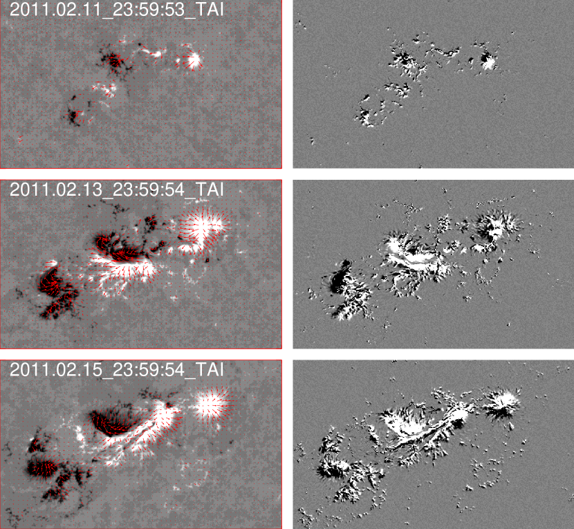
Figure 1.— Photospheric vector magnetograms (left) and plots of $J_{z}B_{z}$ (right) for the active region NOAA 11158 between 11–15 February 2011. The arrows show the transverse component of the magnetic field. Light (dark) shades indicate positive (negative) values of $B_{z}$ on the left and $J_{z}B_{z}$ on the right.

The redistribution of magnetic helicity contained within different scales was argued to be the interchange of twist and writhe due to magnetic helicity conservation (cf. Zeldovich et al., 1983; Kerr & Brandenburg, 1999). Furthermore, the spectral magnetic helicity distribution is important for understanding the operation of the solar dynamo (Brandenburg & Subramanian, 2005a). It has been argued that, if the large-scale magnetic field is generated by an $\alpha$ effect (Krause & Rädler, 1980), it must produce magnetic helicity of opposite signs at large and small length scales (Seehafer, 1996; Ji, 1999). We call such a magnetic field bi-helical (Yousef & Brandenburg, 2003). To alleviate the possibility of catastrophic (magnetic Reynolds number-dependent) quenching of the $\alpha$ effect (Gruzinov & Diamond, 1994) and slow saturation (Brandenburg, 2001), one must invoke magnetic helicity fluxes from small-scale magnetic fields (Kleeorin et al., 2000; Blackman & Field, 2000; Brandenburg & Subramanian, 2005a; Brandenburg et al., 2009; Hubbard & Brandenburg, 2012).

In the present paper, we determine the spectrum of magnetic helicity and its relationship with magnetic energy from photospheric vector magnetograms of a solar active region. We use a technique that is based on the spectral representation of the magnetic two-point correlation tensor. It is related to the method of Matthaeus et al. (1982) for determining the magnetic helicity spectrum from in situ measurements of the magnetic field in the solar wind. Their key assumption allowing for the determination of magnetic helicity spectra is that of homogeneity. This technique was recently applied to data from Ulysses to show that the magnetic field at high heliographic latitudes has opposite signs of helicity in the two hemispheres and also at large and small length scales (Brandenburg et al., 2011); see also Warnecke et al. (2011, 2012) for results from corresponding simulations. In the present work, a variant is proposed where we assume local statistical isotropy in the horizontal plane to compute magnetic energy and helicity spectra.

2. Data analysis

We have analyzed data from the solar active region NOAA 11158 during 11–15 February 2011, taken by the Helioseismic and Magnetic Imager (HMI) on board the Solar Dynamics Observatory (SDO). The pixel resolution of the magnetogram is about $0.5^{\prime\prime}$, and the field of view is $250^{\prime\prime}\times 150^{\prime\prime}$. Figure 1 shows photospheric vector magnetograms (left) and the corresponding distribution of $h_{C}^{(z)}=J_{z}B_{z}$ (right) from the vector magnetograms of that active region on different days. Here, $J_{z}=\partial B_{y}/\partial x-\partial B_{x}/\partial y$, and $J_{z}/\mu_{0}$ is the vertical component of the current density in SI units with $\mu_{0}$ being the vacuum permeability, while in cgs units, the current density is $J_{z}c/4\pi$ with $c$ being the speed of light. The superscript ‘$(z)$’ on $h_{C}^{(z)}$ indicates that only the vertical contribution to the current helicity density is available.

It turns out that the mean value of the current helicity density, ${\cal H}_{C}^{(z)}=\langle{h_{C}^{(z)}}\rangle$, is positive and $\approx 2.7$ G² km^-1. Furthermore, as a proxy of the force-free $\alpha$ parameter, we determine $\alpha=J_{z}/B_{z}$, which is on the average $\langle{\alpha}\rangle\approx 2.8\times 10^{-5}$ km^-1. For future reference, let us estimate the current helicity normalized to its theoretical maximum value, henceforth referred to as relative helicity. This is not to be confused with the gauge-invariant magnetic helicity relative to that of an associated potential field (Berger & Field, 1984). Thus, we consider the ratio

$$r_{C}=\langle J_{z}B_{z}\rangle\left/\left(\langle J_{z}^{2}\rangle\langle B_{z}^{2}\rangle\right)^{1/2}\right.$$ (1)

as an estimate for the relative current helicity. For the active region NOAA 11158 we find $r_{C}=+0.034$. This value is based on one snapshot, but similar values have been found at other times.

Let us now turn to the two-point correlation tensor, $\langle B_{i}({\bm{x}},t)\,B_{j}({\bm{x}}+{\bm{\xi}},t)\rangle$, where ${\bm{x}}$ is the position vector on the two-dimensional surface, and angle brackets denote ensemble averaging or, in the present case, averaging over annuli of constant radii, i.e., $|{\bm{\xi}}|={\rm const}$. Its Fourier transform with respect to ${\bm{\xi}}$ can be written as

$$\left\langle\hat{B}_{i}({\bm{k}},t)\hat{B}_{j}^{*}\!({\bm{k}}^{\prime},t)\right\rangle=\Gamma_{ij}({\bm{k}},t)\delta^{2}({\bm{k}}-{\bm{k}}^{\prime}),$$ (2)

where $\hat{B}_{i}({\bm{k}},t)=\int B_{i}({\bm{x}},t)\,e^{i{\bm{k}}\cdot{\bm{x}}}d^{2}x$ is the two-dimensional Fourier transform, the subscript $i$ refers to one of the three magnetic field components, the asterisk denotes complex conjugation, and ensemble averaging will be replaced by averaging over concentric annuli in wavevector space. Following Matthaeus et al. (1982), it is possible to determine the magnetic helicity spectrum from the spectral correlation tensor $\Gamma_{ij}({\bm{k}},t)$ by making the assumption of local statistical isotropy. At the end of this paper we consider the applicability of this assumption in more detail. Considering that $\bm{k}$ defines the only preferred direction in $\Gamma_{ij}$, and that $k_{i}\hat{B}_{i}=0$, the only possible structure of $\Gamma_{ij}({\bm{k}},t)$ is (cf. Moffatt, 1978)

$$\Gamma_{ij}(\bm{k},t)=\frac{2E_{M}(k,t)}{4\pi k}(\delta_{ij}-\hat{k}_{i}\hat{k}_{j})+\frac{iH_{M}(k,t)}{4\pi k}\varepsilon_{ijk}k_{k},$$ (3)

where $\hat{k}_{i}=k_{i}/k$ is a component of the unit vector of $\bm{k}$, $k=|\bm{k}|$ is its modulus with $k^{2}=k_{x}^{2}+k_{y}^{2}$, and $E_{M}(k,t)$ and $H_{M}(k,t)$ are the magnetic energy and magnetic helicity spectra, normalized such that

$${\cal E}_{M}(t)\equiv\frac{1}{2}\langle{\bm{B}^{2}}\rangle\! = \!{\int}^{\infty}_{0}\!\!E_{M}(k,t)\,dk,$$

$${\cal H}_{M}(t)\equiv\langle{\bm{A}\cdot\bm{B}}\rangle\! = \!\int^{\infty}_{0}\!\!H_{M}(k,t)\,dk.$$ (4)

Note that the mean energy density in ${\rm erg}/{\rm cm}^{3}$ is ${\cal E}_{M}/4\pi$. We emphasize that the expression for $\Gamma_{ij}({\bm{k}},t)$ differs from that of Moffatt (1978) by a factor $2k$, because we are here in two dimensions, so the differential for the integration over shells in wavenumber space changes from $4\pi k^{2}\,dk$ to $2\pi k\,dk$.

Note that the magnetic vector potential is not an observable quantity, so the magnetic helicity might not be gauge-invariant. However, if the spatial average is over all space, or if the magnetic field falls off sufficiently rapidly toward the boundaries, both ${\cal H}_{M}(t)$ and $H_{M}(k,t)$ are gauge-invariant. Indeed, with the present analysis, $H_{M}(k,t)$ is manifestly gauge-invariant, because it has been computed directly from the magnetic field as obtained through the photospheric vector magnetogram.

The components of the correlation tensor of the turbulent magnetic field can be written in the form

$$4\pi k{\bf\Gamma}(k,\phi_{k})=$$ (5)

$$\left(\begin{array}[]{ccc}(1-\cos^{2}\phi_{k})2E_{M}&-\sin 2\phi_{k}E_{M}&-ik\sin\phi_{k}H_{M}\\ -\sin 2\phi_{k}E_{M}&(1-\sin^{2}\phi_{k})2E_{M}&\;\;ik\cos\phi_{k}H_{M}\\ ik\sin\phi_{k}H_{M}&-ik\cos\phi_{k}H_{M}&2E_{M}\end{array}\right),$$ (9)

where we have defined the polar angle in wavenumber space, $\phi_{k}={\rm Arctan}(k_{y},k_{x})$, so that $k_{x}=k\cos\phi_{k}$ and $k_{y}=k\sin\phi_{k}$. For brevity, we have also skipped the arguments $k$ and $t$ on $E_{M}(k,t)$ and $H_{M}(k,t)$.

In the following we present shell-integrated spectra. However, because we consider here two-dimensional spectra, they correspond to the power in annuli of radius $k$ and are obtained as

$$2E_{M}(k,t) = 2\pi k\,\mbox{Re}\left\langle\Gamma_{xx}+\Gamma_{yy}+\Gamma_{zz}\right\rangle_{\phi_{k}},$$ (10)

$$kH_{M}(k,t) = 4\pi k\,\mbox{Im}\left\langle\cos\phi_{k}\Gamma_{yz}-\sin\phi_{k}\Gamma_{xz}\right\rangle_{\phi_{k}},$$ (11)

where the angle brackets with subscript $\phi_{k}$ denote averaging over annuli in wavenumber space.

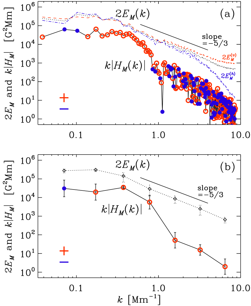
Figure 2.— (a) $2E_{M}(k)$ (dotted line) and $k|H_{M}(k)|$ (solid line) for NOAA 11158 at 23:59:54 UT on 13 February 2011. Positive (negative) values of $H_{M}(k)$ are indicated by open (closed) symbols, respectively. $2E_{M}^{(h)}(k)$ (red, dashed) and $2E_{M}^{(v)}(k)$ (blue, dash-dotted) are shown for comparison. (b) Same as upper panel, but the magnetic helicity is averaged over broad logarithmically spaced wavenumber bins.

The realizability condition (Moffatt, 1969) implies that

$$k|H_{M}(k,t)|\leq 2E_{M}(k,t).$$ (12)

It is therefore convenient to plot $k|H_{M}(k,t)|$ and $2E_{M}(k,t)$ on the same graph, which allows one to judge how helical the magnetic field is at each wavenumber. Furthermore, to assess the degree of isotropy, we also consider magnetic energy spectra $E_{M}^{(h)}(k)$ and $E_{M}^{(v)}(k)$ based respectively on the horizontal and vertical magnetic field components, defined via

$$2E_{M}^{(h)}(k) = 4\pi k\,\mbox{Re}\left\langle\Gamma_{xx}+\Gamma_{yy}\right\rangle_{\phi_{k}},$$ (13)

$$2E_{M}^{(v)}(k) = 4\pi k\,\mbox{Re}\left\langle\Gamma_{zz}\right\rangle_{\phi_{k}}.$$ (14)

Under isotropic conditions, we expect $E_{M}(k)\approx E_{M}^{(h)}(k)\approx E_{M}^{(v)}(k)$.

We now consider magnetic energy and helicity spectra for the active region NOAA 11158. The calculated region of the field of view is $256^{\prime\prime}\times 256^{\prime\prime}$, i.e. $512\times 512$ pixels or $L^{2}=(186\,{\rm Mm})^{2}$. We present first the results for NOAA 11158 at 23:59:54UT on 13 February 2011; see Figure 2(a). It turns out that the magnetic energy spectrum has a clear $k^{-5/3}$ range for wavenumbers in the interval $0.5\,{\rm Mm}^{-1}<k<5\,{\rm Mm}^{-1}$. The magnetic helicity spectrum is predominantly positive at intermediate wavenumbers, but we also see that toward high wavenumbers the magnetic helicity is fluctuating strongly around small values. To determine the sign of magnetic helicity at these smaller scales, we average the spectrum over broad, logarithmically spaced wavenumber bins; see the lower panel of Figure 2. This shows that even at smaller length scales the magnetic helicity is still positive, again consistent with the fact that this active region is at southern latitudes.

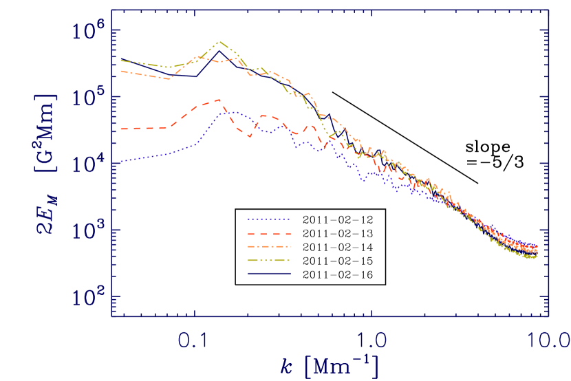
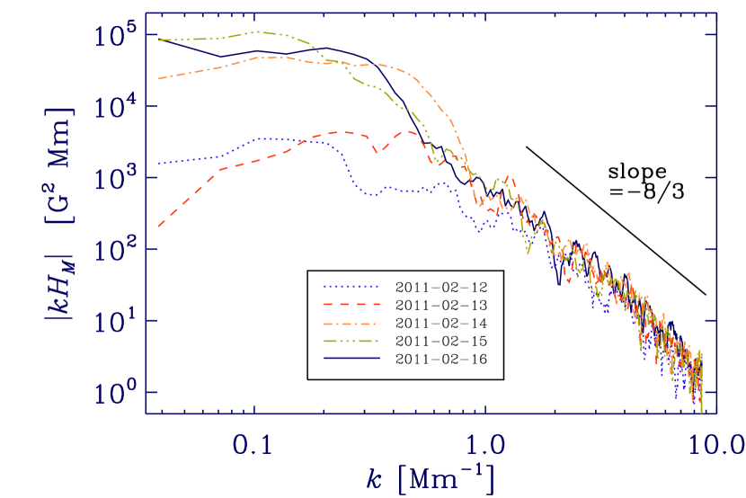
Figure 3.— Similar to Figure 2, showing $E_{M}(k,t)$ (upper panel) and $k|H_{M}(k,t)|$ (lower panel) for the other days.

To calculate the relative magnetic helicity $r_{M}$, we define the integral scale of the magnetic field in the usual way as

$$\ell_{M}=\left.\int k^{-1}E_{M}(k)\,dk\right/\int E_{M}(k)\,dk.$$ (15)

The realizability condition of Equation (12) can be rewritten in integrated form (e.g. Kahniashvili et al., 2013) as

$$|{\cal H}_{M}|=\left|\int\!H_{M}dk\right|\leq 2\!\int\!k^{-1}E_{M}(k)dk\equiv 2\ell_{M}{\cal E}_{M}.\quad$$ (16)

In particular, we have $|{\cal H}_{M}(t)|\leq 2\ell_{M}{\cal E}_{M}(t)$. This gives

$$r_{M}={\cal H}_{M}/2\ell_{M}{\cal E}_{M},$$ (17)

which obeys $|r_{M}|\leq 1$. Again, this quantity is not to be confused with the gauge-invariant helicity of Berger & Field (1984). For the active region NOAA 11158 at 23:59:54 UT on 13 February 2011 we have $\ell_{M}\approx 5.8\,{\rm Mm}$, ${\cal H}_{M}\approx 3.3\times 10^{4}\,{\rm G}^{2}\,{\rm Mm}$, and ${\cal E}_{M}\approx 6.7\times 10^{4}\,{\rm G}^{2}$, so $r_{M}\approx 0.042$. The relative magnetic helicity has thus the same sign as the relative current helicity. The corresponding magnetic column energy in the two-dimensional domain of size $L^{2}$ is $L^{2}{\cal E}_{M}/4\pi\approx 1.8\times 10^{24}\,{\rm erg}\,{\rm cm}^{-1}$, which is about three times larger than the values given by Song et al. (2013). The magnetic column helicity is $L^{2}{\cal H}_{M}\approx 1.1\times 10^{33}\,{\rm Mx}^{2}\,{\rm cm}^{-1}$. Several estimates of the gauge-invariant magnetic helicity of NOAA 11158 using time integration of photospheric magnetic helicity injection (Vemareddy et al., 2012; Liu & Schuck, 2012) and nonlinear force-free coronal field extrapolation (Jing et al., 2012; Tziotziou et al., 2013) suggest magnetic helicities of the order of $10^{43}\,{\rm Mx}^{2}$. This value would be comparable to ours if the effective vertical extent were $\approx 100\,{\rm Mm}$. We should remember, however, that there is no basis for such a vertical extrapolation of our two-dimensional data.

Interestingly, the magnetic energy spectra $E_{M}^{(h)}(k)$ and $E_{M}^{(v)}(k)$ based respectively on the horizontal and vertical magnetic field components agree remarkably well at wavenumbers below $k=3\,{\rm Mm}^{-1}$, corresponding to length scales larger than 2 Mm. This suggests that our assumption of isotropy might be a reasonable one. The mutual departure between $E_{M}^{(h)}(k)$ and $E_{M}^{(v)}(k)$ at larger wavenumbers could in principle be a physical effect, although there is no good reason why the magnetic field should be mostly vertical only at small scales. If it is indeed a physical effect, it should then in future be possible to verify that this wavenumber, where $E_{M}^{(h)}(k)$ and $E_{M}^{(v)}(k)$ depart from each other, is independent of the instrument. Alternatively, this departure might be connected with different accuracies of horizontal and vertical magnetic field measurements (Zhang et al., 2012). If that is the case, one should expect that with future measurements at better resolution the two spectra depart from each other at larger wavenumbers. In that case, our spectral analysis could be used to isolate potential artefacts in the determination of horizontal and vertical magnetic fields.

In Figure 3 we show $2E_{M}(k)$ and $k|H_{M}(k)|$ for different days. It turns out that on small scales the spectra are rather similar in time, and that there are differences in the amplitude mainly on large scales. Also the sign of $H_{M}(k)$ remains positive for the different days.

We find that the mean spectral values of magnetic energy of the active region at the solar surface is consistent with a $k^{-5/3}$ power law, which is expected based on the theory of Goldreich and Sridhar (1995) and consistent with spectra from earlier work on solar magnetic fields (Abramenko, 2005; Stenflo, 2012), ruling out the $k^{-3/2}$ spectrum suggested by Iroshnikov (1963) and Kraichnan (1965).

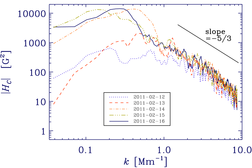
Figure 4.— Unsigned current helicity spectrum, $|H_{C}(k)|$.

Under isotropic conditions, the current helicity spectrum, $H_{C}(k,t)$, is related to the magnetic helicity spectrum via (Moffatt, 1978)

$$H_{C}(k,t)\approx k^{2}H_{M}(k,t).$$ (18)

It is normalized such that $\int H_{C}(k)\,dk=\langle\bm{J}\cdot\bm{B}\rangle$. In Figure 4 we show $|H_{C}(k)|$ obtained in this way. For $k\gtrsim 1{\rm Mm}^{-1}$, the current helicity spectrum shows a $k^{-5/3}$ spectrum, which is consistent with numerical simulations of helically forced hydromagnetic turbulence (Brandenburg and Subramanian, 2005b; Brandenburg, 2009), and indicative of a forward cascade of current helicity. Similar spectra have also been obtained for the analogous case of kinetic helicity (André & Lesieur, 1977; Borue & Orszag, 1997). These results imply that the relative helicity decreases toward smaller scales; see the corresponding discussion on p. 286 of Moffatt (1978).

3. Conclusions

We have applied a novel technique to estimate the magnetic helicity spectrum using vector magnetogram data at the solar surface. We have made use of the assumption that the spectral two-point correlation tensor of the magnetic field can be approximated by its isotropic representation. This assumption is partially justified by the fact that the energy spectra from horizontal and vertical magnetic fields agree at wavenumbers below $2\,{\rm Mm}^{-1}$. However, it will be important to assess the assumption of isotropy in future work through comparison with simulations. An example are the simulations of Losada et al. (2013), who employed however only a one-dimensional representation of the spectral two-point correlation function. Nevertheless, the present results look promising, because the sign of magnetic helicity is the same over a broad range of wavenumbers and consistent with that theoretically expected for the southern hemisphere. This is consistent with the right-handed twist inferred from all previous studies of NOAA 11158 using different methods. Except for the smallest wavenumbers, magnetic and current helicities have essentially the same sign. Therefore, a sign change is only expected at smaller wavenumbers corresponding to scales comparable to those of the Sun itself.

It would be useful to extend our analysis to a larger surface area of the Sun to see whether there is evidence for a sign change toward small wavenumbers and thus large scales reflecting the global magnetic field of the solar cycle. Such a change of sign is expected from dynamo theory (Brandenburg, 2001) and is a consequence of the inverse cascade of magnetic helicity (Pouquet et al., 1976). Figure 2 gives indications of an opposite sign for $k\leq 0.1\,{\rm Mm}^{-1}$, which corresponds to scales that are still much smaller than those of the Sun. However, measurements of spectral power on scales comparable to those of the observed magnetogram itself are not sufficiently reliable.

Our results suggest that the unsigned current helicity spectrum shows a $k^{-5/3}$ power law. This is in agreement with simulations of hydromagnetic turbulence (Brandenburg and Subramanian, 2005b) and implies that the turbulence becomes progressively less helical toward smaller scales. Our results suggest that at a typical scale of $\ell_{M}\approx 6\,$Mm, the relative magnetic helicity reaches values around $0.04$. This magnetic helicity must have its origin in the underlying dynamo process, and can be traced back to the interaction between rotation and stratification. Losada et al. (2013) parameterized these two effects in terms of a stratification parameter Gr and a Coriolis number Co and found that the relative kinetic helicity is approximately 2 Gr Co. For the Sun, they estimate ${\rm Gr}=1/6.5$, so a relative helicity of 0.04 might correspond to ${\rm Co}\approx 0.1$. For the solar rotation rate, this corresponds to a correlation time of about 6 hours, which translates to a depth of about 8 Mm. Again, more precise estimates should be obtained using realistic simulations.

In addition to measuring magnetic helicity over larger regions, it will be important to apply our technique to many active regions covering both hemispheres of the Sun and different times during the solar cycle. This would allow us to verify the expected hemispheric dependence of magnetic helicity. Compared with previous determinations of the hemispheric dependence of current helicity (Zhang et al., 2012), our technique might allow us to isolate instrumental artefacts resulting from different resolutions of vector magnetograms for horizontal and vertical magnetic fields.

References

- Abramenko et al. (1997) Abramenko, V. I., Wang, T., & Yurchishin, V. B. 1997, SoPh, 174, 291
- Abramenko (2005) Abramenko, V. I. 2005, ApJ, 629, 1141
- André & Lesieur (1977) André, J.-C., & Lesieur, M. 1977, JFM, 81, 187
- Berger & Field (1984) Berger, M. A., & Field, G. B. 1984, JFM 147, 133
- Blackman & Field (2000) Blackman, E. G., & Field, G. B. 2000, ApJ, 534, 984
- Borue & Orszag (1997) Borue, V., & Orszag, S. A. 1997, PhRvE, 55, 7005
- Brandenburg (2001) Brandenburg, A. 2001, ApJ, 550, 824
- Brandenburg (2009) Brandenburg, A. 2009, ApJ, 697, 1206
- Brandenburg & Subramanian (2005a) Brandenburg, A., & Subramanian, K. 2005a, PhR, 417, 1
- Brandenburg and Subramanian (2005b) Brandenburg, A., & Subramanian, K. 2005b, A&A, 439, 835
- Brandenburg et al. (2009) Brandenburg, A., Candelaresi, S., & Chatterjee, P. 2009, MNRAS, 398, 1414
- Brandenburg et al. (2011) Brandenburg, A., Subramanian, K., Balogh, A., & Goldstein, M. L. 2011, ApJ, 734, 9
- Chae (2001) Chae, J. 2001, ApJ, 560, L95
- Goldreich and Sridhar (1995) Goldreich, P., & Sridhar, S. 1995, ApJ, 438, 763
- Gruzinov & Diamond (1994) Gruzinov, A. V., & Diamond, P. H. 1994, PhRvL, 72, 1651
- Hubbard & Brandenburg (2012) Hubbard, A., & Brandenburg, A. 2012, ApJ, 748, 51
- Iroshnikov (1963) Iroshnikov, R. S. 1963, Sov. Astron., 7, 566
- Ji (1999) Ji, H. 1999, PhRvL, 83, 3198
- Jing et al. (2012) Jing, J., Park, S.-H., Liu, C., Lee, J., Wiegelmann, T., Xu, Y., Deng, N., & Wang, H. 2012, ApJ, 752, L9
- Kahniashvili et al. (2013) Kahniashvili, T., Tevzadze, A. G., Brandenburg, A., & Neronov, A. 2013, PhRvD, 87, 083007
- Kerr & Brandenburg (1999) Kerr, R. M., & Brandenburg, A. 1999, PhRvL, 83, 1155
- Kleeorin et al. (1995) Kleeorin, N., & Rogachevskii, I. 1999, PhRvE, 59, 6724
- Kleeorin et al. (2000) Kleeorin, N., Moss, D., Rogachevskii, I., & Sokoloff, D. 2000, A&A, 361, L5
- Kraichnan (1965) Kraichnan, R. H. 1965, Phys. Fluids, 8, 1385
- Krause & Rädler (1980) Krause, F., & Rädler, K.-H. 1980, Mean-field Magnetohydrodynamics and Dynamo Theory (Oxford: Pergamon Press)
- Liu & Schuck (2012) Liu, Y., & Schuck, P. W. 2012, ApJ, 761, 105
- Losada et al. (2013) Losada, I. R., Brandenburg, A., Kleeorin, N., & Rogachevskii, I. 2013, A&A, 556, A83
- Matthaeus et al. (1982) Matthaeus, W. H., Goldstein, M. L., & Smith, C. 1982, PhRvL, 48, 1256
- Moffatt (1969) Moffatt, H. K. 1969, JFM, 35, 117
- Moffatt (1978) Moffatt, H. K., Magnetic field generation in electrically conducting fluids, 1978, Cambridge University Press, Cambridge
- Pevtsov et al. (1994) Pevtsov, A. A., Canfield, R. C., & Metcalf, T. R. 1994, ApJ, 425, L117
- Pouquet et al. (1976) Pouquet, A., Frisch, U., & Léorat, J. 1976, JFM, 77, 321
- Seehafer (1990) Seehafer, N. 1990, SoPh, 125, 219
- Seehafer (1996) Seehafer, N. 1996, PhRvE, 53, 1283
- Song et al. (2013) Song, Q., Zhang, J., Yang, S.-H., Liu, Y. 2013, RAA, 13, 226
- Stenflo (2012) Stenflo, J. O. 2012, A&A, 541, A17
- Su et al. (2009) Su, J. T., Sakurai, T., Suematsu, Y., Hagino, M., & Liu, Y. 2009, ApJ, 697, L103
- Taylor (1986) Taylor, J. B. 1986, RvMP, 58, 741
- Tziotziou et al. (2013) Tziotziou, K., Georgoulis, M. K., & Liu, Y. 2013, ApJ, 772, 115
- Vemareddy et al. (2012) Vemareddy, P., Ambastha, A., Maurya, R. A., & Chae, J. 2012, ApJ, 761, 86
- Venkatakrishnan & Tiwari (2009) Venkatakrishnan, P., & Tiwari, S. 2009, ApJ, 706, L114
- Warnecke et al. (2011) Warnecke, J., Brandenburg, A., & Mitra, D. 2011, A&A, 534, A11
- Warnecke et al. (2012) Warnecke, J., Brandenburg, A., & Mitra, D. 2012, JSWJC, 2, A11
- Woltjer (1958a) Woltjer, L. 1958a, PNAS, 44, 489
- Woltjer (1958b) Woltjer, L. 1958b, PNAS, 44, 833
- Yousef & Brandenburg (2003) Yousef, T. A., & Brandenburg, A. 2003, A&A, 407, 7
- Zeldovich et al. (1983) Zeldovich, Y. B., Ruzmaikin, A. A., & Sokoloff, D. D., 1983, Magnetic fields in astrophysics, New York, Gordon and Breach
- Zhang (2010) Zhang, H. 2010, ApJ, 716, 1493
- Zhang et al. (2012) Zhang, H., Moss, D., Kleeorin, N., Kuzanyan, K., Rogachevskii, I., Sokoloff, D., Gao, Y., & Xu, H. 2012, ApJ, 751, 47