Fermionized photons in the ground state of one-dimensional coupled cavities

Abstract

The Density Matrix Renormalization Group algorithm is used to characterize the ground states of one-dimensional coupled cavities in the regime of low photon densities. Numerical results for photon and spin excitation densities, one- and two-body correlation functions, superfluid and condensate fractions, as well as the entanglement entropy and localizable entanglement are obtained for the Jaynes-Cummings-Hubbard (JCH) model, and are compared with those for the Bose-Hubbard (BH) model where applicable. The results indicate that a Tonks-Girardeau phase, in which the photons are strongly fermionized, appears between the Mott-insulating and superfluid phases as a function of the inter-cavity coupling. In fact, the superfluid density is found to be zero in a wide region outside the Mott-insulator phase boundary. The presence of two different species of excitation (spin and photon) in the JCH model gives rise to properties with no analog in the BH model, such as the (quasi)condensation of spin excitations and the spontaneous generation of entanglement between the atoms confined to each cavity.

I Introduction

The idea of simulating a complex, many-body physical system with a simpler model system has a long and rich history. A prominent example is the Bose-Hubbard (BH) model Fisher et al. (1989), which governs the dynamics of bosons tunneling between sites of a lattice with energy $t$ and interacting on a given site with energy $U$. Originally proposed to describe the behavior of superfluid ⁴He in porous Vycor glass, it is now applied to a plethora of experimental systems including Josephson junction arrays van der Zant et al. (1992), ultracold atoms in optical lattices Bloch (2005), photonic crystals Corrielli et al. (2013), and arrays of coupled cavities Hartmann et al. (2006); Greentree et al. (2006); Angelakis et al. (2007); Houck et al. (2012).

For repulsive interactions ($U>0$), there is a competition between delocalization due to the tunneling and the tendency to localize due to the energy cost of multiple occupancy of a given site. As a consequence, the model exhibits a quantum (zero-temperature) phase transition Fisher et al. (1989). In the strongly interacting (weak tunneling) regime $t/U\ll 1$, the ground state is predicted to be a Mott insulator (MI) Mott and Peierls (1937); Mott (1949, 1982), in which each site is occupied by an (identical) integer number of bosons; for $t/U\gg 1$, a superfluid (SF) state results Kapitza (1938); Allen and Misener (1938); Landau (1941), in which the bosons become completely delocalized. The transition between these phases was first realized in Bose-Einstein condensates confined in three-dimensional optical lattice potentials Greiner et al. (2002), where the ratio $t/U$ was controlled by varying the well depth, and subsequently observed in many other cold-atom optical lattice experiments in one, two and three dimensions Stöferle et al. (2004); Spielman et al. (2007); Gemelke et al. (2009); Bakr et al. (2010); Haller et al. (2010); Trotzky et al. (2010).

There has been much recent interest in observing similar quantum phase transitions in cavity quantum electrodynamics Hartmann et al. (2006); Greentree et al. (2006); Angelakis et al. (2007). The principal motivation for employing these environments is the robustness of available technology for producing, manipulating and detecting photons. Unfortunately, photons do not intrinsically interact. Various strategies have been proposed to overcome this limitation, and a vast array of interesting many-body states have been conjectured to appear as a result Hartmann et al. (2007); Rossini and Fazio (2007); Carusotto et al. (2009); Kiffner and Hartmann (2010); Halu et al. (2013); Hayward et al. (2012); Schiró et al. (2012). One model that has attracted particular attention is the Jaynes-Cummings-Hubbard (JCH) model Hartmann et al. (2006, 2008); Makin et al. (2008), comprising a lattice of high-finesse optical cavities each containing one or more two-level atoms, with neighboring cavities coupled via the overlap of their evanescent modes. The (bosonic) photons can then be considered to ‘tunnel’ from cavity to cavity. The atom interacts with the quantized electromagnetic field present within the cavity according to the Jaynes-Cummings model Jaynes and Cummings (1963), and photon interactions are generated via the photon-blockade mechanism Birnbaum et al. (2005). Importantly, the lattice polaritons that constitute the spin-photon elementary excitations of the JCH model are also expected to undergo a phase transition from a Mott insulator to a superfluid Greentree et al. (2006); Hartmann et al. (2006); Angelakis et al. (2007); Rossini and Fazio (2007); Aichhorn et al. (2008); Koch and LeHur (2009); Schmidt and Blatter (2009); Pippan et al. (2009); Schmidt and Blatter (2010); Knap et al. (2010); Hohenadler et al. (2011). While early proposals for the experimental realization of coupled cavities involved nitrogen vacancies in diamond Greentree et al. (2006), self-assembled quantum dots in photonic crystals Na et al. (2008), and trapped ions Ivanov et al. (2009); Mering et al. (2009), more recent proposals favor circuit QED Nunnenkamp et al. (2011); Wu et al. (2011); Houck et al. (2012); Schmidt and Koch (2013).

The close similarity between the properties of the BH and JCH models suggests that the polariton superfluid resulting from arranging cavities along a row should be rather peculiar. In one dimension, the interaction energy of free bosons is strongly enhanced relative to their kinetic energy at low densities Bloch (2005), a result that will be discussed in greater detail in Sec. II.3. The resulting Tonks-Girardeau gas Tonks (1936); Girardeau (1960) is described as the hard-core limit of the (integrable) Lieb-Liniger model for bosons with delta-function interactions in one dimension Lieb and Liniger (1963). These hard-core bosons can be exactly mapped to non-interacting fermions Girardeau (1960); for general densities the state is well-described within the framework of Luttinger liquid theory Giamarchi (2003). The Tonks-Girardeau gas was first realized in ultracold atomic Bose gases confined in one-dimensional optical lattices Paredes et al. (2004); Kinoshita et al. (2004). More recently, the transition between a Luttinger liquid and Mott-insulating state was observed Haller et al. (2010). These results suggest that a one-dimensional arrangement of coupled cavities should be sufficient to induce the mobile photons to behave entirely as fermions. In fact, this possibility was noted previously for a dissipative model Carusotto et al. (2009). The central goal of the present investigation is to show that the photons are effectively fermionized in the ground-state of the JCH model. A secondary goal is to make a careful, side-by-side comparison of the JCH and BH models in one dimension.

In this work, the ground states of the zero-temperature one-dimensional JCH and BH models in the vicinity of the MI phase boundary are obtained numerically using finite-system density matrix renormalization group (DMRG) methods. Several quantities are calculated that provide evidence for the nature of the states, including particle densities, one-particle and two-particle correlation functions, the superfluid fraction, the condensate fraction, and the entanglement entropy. Finite-size scalings are performed in order to infer the value of these quantities in the thermodynamic limit.

Two main conclusions can be drawn from our work. First, for small cavity couplings the ground state consists of a polariton MI phase as expected, though with some interesting features not shared by single-component Bose systems. Second, the results clearly reveal the strong fermionization of both the photons and spins in the JCH system throughout the so-called superfluid phase in the low-density limit. Detailed comparisons are made with the ground states of the BH model in the equivalent parameter regimes. The main conclusion that can be drawn is that superfluidity is weakly manifested in this phase, if it exists at all.

The manuscript is organized as follows. The JCH and BH models are reviewed in Sec. II, and the DMRG methods used in the characterization of their ground states is described. This section also discusses the properties of the Tonks-Girardeau gas. The numerical results are presented in Sec. III, and the discussion and conclusions are found in Sec. IV.

II Models and Methods

In this work we compare the properties of the one-dimensional Jaynes-Cummings-Hubbard (JCH) and Bose-Hubbard (BH) models, using density matrix renormalization group (DMRG) methods. This section briefly provides the background to these models and describes the numerical methods employed in the calculations.

II.1 JCH model

The behavior of a single two-level atom, in the pseudospin representation, confined to a single high-finesse cavity is given by the Jaynes-Cummings Hamiltonian Jaynes and Cummings (1963), written within the rotating-wave approximation Mandel and Wolf (1995) as

$$H_{\rm JC}=\omega_{c}\left(a^{{\dagger}}a+\frac{1}{2}\right)+\frac{1}{2}\omega_{a}\sigma^{z}+g\left(a^{{\dagger}}\sigma^{-}+a\sigma^{+}\right).$$ (1)

Here, $\omega_{c}$ is the natural cavity frequency ($\hbar=1$ in this work for convenience), $\omega_{a}$ is the excitation frequency of the atom, $a$ ($a^{{\dagger}}$) is the photon annihilation (creation) operator, $\sigma^{z}$ is the spin-$1/2$ representation of the Pauli $z$ operator, $\sigma^{\pm}$ are the spin raising and lowering operators, and $g$ is the strength of the atom-photon coupling, proportional to the magnitude of the inner product between the dipole vector and the local field. In this work, $g$ is assumed to be a real quantity, equivalent to assuming that the dipole and field oscillate in phase. This model describes an isolated system which ignores environmental couplings. The cavity is therefore assumed to have arbitrarily high finesse, and be in the strong-coupling limit.

In the rotating-wave approximation the total number of excitations

$$N_{i}=a_{i}^{{\dagger}}a_{i}+\sigma^{+}_{i}\sigma^{-}_{i},$$ (2)

is a conserved quantity (note that the spin number operator would normally contribute the term $\sigma^{-}_{i}\sigma^{+}_{i}$, but this corresponds to the population of atoms in the ground state; hence, it is not included in the excitation number operator). The eigenstates of $H_{\mathrm{JC}}$ are coherent superpositions of photonic and spin excitations with a definite total excitation number, known as polaritons Hartmann et al. (2006). Within a particular excitation number block $N$, the eigenstates are given (c.f. Appendix A of Ref. Koch and LeHur (2009)) by

$$|N-\rangle=\sin{\theta_{N}}|Ng\rangle+\cos{\theta_{N}}|(N-1)e\rangle;$$ (3)

$$|N+\rangle=\cos{\theta_{N}}|Ng\rangle-\sin{\theta_{N}}|(N-1)e\rangle,$$ (4)

with mixing angle

$$\theta_{N}=\frac{1}{2}\arctan{\left(\frac{2g\sqrt{N}}{\delta}\right)}.$$ (5)

Here $\delta:=\omega_{c}-\omega_{a}$ is the detuning of the cavity and atomic frequencies. The eigenenergies of Eq. (1) for $N\geq 1$ are given by

$$E_{N\pm}=N\omega_{c}+\frac{\delta}{2}\pm\left[\left(\frac{\delta}{2}\right)^{2}+Ng^{2}\right]^{1/2},$$ (6)

while for $N=0$, $E_{0}=0$. The energy levels are thus arranged in two-dimensional manifolds labeled by the polariton number $N$ (except for the $N=0$ sector, which is one-dimensional), separated by the energy of the single-photon cavity mode, $\omega_{c}$.

The anharmonicity in the eigenenergies (6) of size $\sqrt{N}$ is the origin of the photon-blockade effect Birnbaum et al. (2005), giving rise to effective photon interactions. Consider for simplicity the zero-detuning case $\delta=0$ giving eigenenergies $E_{N\pm}=N\omega_{c}\pm g\sqrt{N}$. With one photon the cavity has the lower energy eigenvalue $E_{1-}=\omega_{c}-g$. Naïvely, two independent photons would yield the total energy $2E_{1-}=2\omega_{c}-2g$, but in fact the two-photon energy eigenvalue is $E_{2-}=2\omega_{c}-g\sqrt{2}$. The difference between these energies yields an estimate for the effective repulsive photon-photon interaction strength: $E_{2-}-2E_{1-}=(2-\sqrt{2})g$.

In the Jaynes-Cummings-Hubbard (JCH) model, the cavity mode leakage is no longer neglected. Instead, one imagines a regular lattice of $L^{d}$ cavities in $d$ dimensions positioned sufficiently close together that a photon emitted from one cavity can be absorbed into an adjacent cavity with energy (rate) $\kappa$. The JCH model is written as

$$H_{\mathrm{JCH}}=\displaystyle\sum_{i}\left(H_{\mathrm{JC},i}-\mu N_{i}\right)-\kappa\sum_{\langle i,j\rangle}\left(a^{{\dagger}}_{i}a_{j}+a^{{\dagger}}_{j}a_{i}\right),$$ (7)

where $H_{{\rm JC},i}$ and $N_{i}$ are Eqs. (1) and (2) respectively with $\{a,a^{{\dagger}},\sigma^{z},\sigma^{\pm}\}$ replaced by $\{a_{i},a^{{\dagger}}_{i},\sigma^{z}_{i},\sigma^{\pm}_{i}\}$, and $i$ labels the position of a cavity. The $\langle i,j\rangle$ notation indicates that the sum is over nearest neighbors. The chemical potential $\mu$ fixes the mean polariton number, and is employed primarily to connect with the results of the BH model which is generally solved in the grand canonical ensemble. Note that in the JCH model, the atoms are fixed within the cavities, and only the photons are able to ‘tunnel’ from cavity to adjacent cavity.

For reasons that will become clearer momentarily, it is convenient to rescale the JCH energy in units of the coupling constant $g$; in the limit of zero detuning $\omega_{c}=\omega_{a}$ one can rewrite the Hamiltonian (7) as

$$\frac{H_{\rm JCH}}{g} = -\frac{\kappa}{g}\sum_{\langle i,j\rangle}\left(a_{i}^{{\dagger}}a_{j}+a_{j}^{{\dagger}}a_{i}\right)$$ (8)

$$+ \sum_{i}\left[a_{i}^{{\dagger}}\sigma_{i}^{-}+a_{i}\sigma_{i}^{+}-\left(\frac{\mu-\omega_{c}}{g}\right)N_{i}\right],$$

where unimportant additive constant terms are omitted. The first term corresponds to the photon hopping, the second to the local JC term, and the last term can be considered as a rescaled chemical potential for the total polariton density $\tilde{\mu}:=(\mu-\omega_{c})/g$.

II.2 BH Model

In the BH model, bosons tunnel between nearest neighboring sites of a lattice, and experience on-site interactions (which can be either attractive or repulsive in general). The model is described by the Hamiltonian

$$H_{\mathrm{BH}}=-t\sum_{\langle i,j\rangle}\left(b^{{\dagger}}_{i}b_{j}+b^{{\dagger}}_{j}b_{i}\right)+\sum_{i}\left[\frac{U}{2}N_{i}(N_{i}-1)-\mu N_{i}\right],\$$ (9)

where $b_{i}$, $b^{{\dagger}}_{i}$, and $N_{i}:=b^{{\dagger}}_{i}b_{i}$ are respectively the bosonic annihilation, creation, and number operators for site $i$, $t>0$ is the nearest-neighbor tunneling amplitude and $U$ is the on-site interaction energy. The chemical potential fixes the mean boson density on the lattice. In this work only repulsive interactions $U>0$ will be considered.

While a direct mapping between the JCH and BH models is not possible because the former has two different kinds of excitations while the latter has only one, the parameters can be chosen in such a way as to simplify comparisons. One can rescale the BH energies in terms of the interaction strength by dividing Eq. (9) by $U$. In this case the hopping amplitudes are $\kappa/g$ and $t/U$ in the JCH and BH models, respectively. The effective interaction strength between photons is $(2-\sqrt{2})g$, which implies that the two systems should become similar for $t/U\sim\kappa/(2-\sqrt{2})g=\left(1+\frac{1}{\sqrt{2}}\right)(\kappa/g)\approx 1.707(\kappa/g)$. A similar connection can be obtained between the chemical potentials of the two models: $\tilde{\mu}+1\sim(2-\sqrt{2})\mu/U$ or $\mu/U\sim 1.707(\tilde{\mu}+1)$. Note that these scalings are valid only when only a single atom is confined to each cavity.

As discussed in the Introduction, in the weak tunneling (strong interactions) limit $t/U\ll 1$ the ground state is an incompressible MI characterized by localized bosons, (constant) integer occupation of a given site, and an energy gap to excitations of order $U$. Deep in this limit, the ground-state wavefunction can be approximated as $|\Psi\rangle\sim\prod_{i}b_{i}^{{\dagger}}|\Phi\rangle$, where $|\Phi\rangle$ is the particle vacuum state and the product is over all lattice sites. Because each site is independent of any other, the overlap of the states $b_{s}|\Psi\rangle$ and $b_{r}|\Psi\rangle$ is exactly zero unless $r=s$. The one-body boson correlation function

$$G^{(1)}(r,s)=\langle b_{r}^{{\dagger}}b_{s}\rangle$$ (10)

and the two-body correlation function

$$G^{(2)}(r,s)=\langle b_{r}^{{\dagger}}b_{s}^{{\dagger}}b_{s}b_{r}\rangle$$ (11)

will then be zero for all $r\neq s$. In reality, for any finite $t/U$ the gapped ground state will deviate from this simple prediction and the correlation functions should instead decrease exponentially in $|r-s|$ with a characteristic length scale $\xi\sim 1/U$ that scales as the inverse of the gap to excitations Hastings and Koma (2006). The correlation length diverges as a system becomes critical Sachdev (2000). One would therefore expect $\xi$ to increase from $0$ to $\infty$ as the hopping goes from 0 to its critical value at the phase boundary for a fixed chemical potential.

The phase boundary in $\mu$-$t$ space, known as the ‘Mott lobe,’ is roughly semi-circular in profile in two and three dimensions Fisher et al. (1989). For $\mu\notin\mathbb{Z}$, the system remains in the MI phase with increasing $t$ until some critical value at which point the system undergoes a phase transition to SF; likewise for constant $t$ and increasing $\mu$. The Mott lobe becomes strongly distorted in one dimension Kühner and Monien (1998), and the system displays re-entrance: at constant $\mu$, on increasing $t$ the ground state phase changes from MI to SF to MI and back to SF again.

In the strong tunneling (weak interactions) limit $t/U\gg 1$, the ground state of the BH model corresponds to an interacting Bose-Einstein condensate. Each boson is highly extended throughout the lattice, and the ground state can be approximated by $|\Psi\rangle\sim\left(\sum_{i}b_{i}^{{\dagger}}\right)^{N_{B}}|\Phi\rangle$, where $N_{B}$ is the number of bosons. This compressible state is characterized by a gapless linear spectrum and long-range correlation functions (10) and (11) that are independent of $|r-s|$. In one-dimension, however, true Bose-Einstein condensation is not possible; rather, the ground state corresponds to a quasi-condensate with only algebraic long-finite order and characterized by strong fluctuations Popov (1987). Instead one finds $G^{(1)}(r,s)\sim 1/|r-s|^{\alpha}$, where the parameter $\alpha$ characterizes the degree of quasi-condensation ($\alpha\to 0$ for a true condensate).

II.3 Tonks-Girardeau Gas

At very low densities, one-dimensional repulsively interacting bosons form a Tonks-Girardeau gas, and effectively behave as non-interacting fermions Girardeau (1960). In the absence of any external potential (other than the ones used for confinement), the ground state properties are governed by the kinetic and interaction potential energies $T$ and $U$. The mean kinetic energy per particle scales as $T/N\sim 1/m\ell^{2}\sim\langle n\rangle^{2}/m$, where $\ell$ is the mean interparticle distance which in one dimension scales as the inverse of the mean particle density $\ell\sim 1/\langle n\rangle$. (In the presence of a weak lattice, the bare boson mass $m$ is rescaled to an effective mass $m^{*}\sim 1/t$). When the interaction potential can be modeled in terms of a pseudopotential (low energy, long-wavelength collisions), one can write the mean interaction potential in one dimension as $U/N\sim\langle n\rangle/m|a_{\rm 1D}|$ Olshanii (1998), where $a_{\rm 1D}$ is the one-dimensional s-wave scattering length. The Tonks parameter, the ratio of the potential and kinetic energies $\gamma=U/T=2/\langle n\rangle|a_{\rm 1D}|$ is therefore huge at low densities, in marked contrast to the situation in higher dimensions. To minimize the interaction potential, particles prefer to be as far apart from one another as possible, much like fermions.

The free fermionic wavefunction can be written in terms of a Slater determinant to guarantee the proper antisymmetrization of the wavefunction. For example, a system of $N$ free fermions on $L$ sites has a wavefunction given in the position representation by

$$\Psi_{F}(r_{1},\dots,r_{L})=\text{det}\left[\begin{array}[]{cccc}\phi_{1}(r_{1})&\phi_{1}(r_{2})&\dots&\phi_{1}(r_{L})\\ \phi_{2}(r_{1})&\phi_{2}(r_{2})&\dots&\phi_{2}(r_{L})\\ \vdots&\vdots&\ddots&\vdots\\ \phi_{N}(r_{1})&\phi_{N}(r_{2})&\dots&\phi_{N}(r_{L})\end{array}\right],$$ (12)

where the $\left\{r_{i}\right\}$ indicate the positions of the lattice sites and the $\left\{\phi_{i}\right\}$ are single-particle wavefunctions. In the perfectly hard-core limit of the Tonks-Girardeau gas, the ground state of the fermionized bosons is simply

$$\Psi_{B}(r_{1},\dots,r_{L})=\prod_{i<j}^{L}{\rm sgn}(r_{i}-r_{j})\Psi_{F}(r_{1},\dots,r_{L}),$$ (13)

where the factor multiplying $\Psi_{F}$ ensures that all negative signs associated with the interchange of two fermions disappears.

Many properties are shared by $\Psi_{F}$ and $\Psi_{B}$. For example, the local density profile of both systems in real space is the same, since $|\Psi_{B}(r_{1},\dots,r_{N})|^{2}=|\Psi_{F}(r_{1},\dots,r_{N})|^{2}$ Yukalov and Girardeau (2005). Similarly, all density correlation functions are the same Cazalilla et al. (2011); for example, for a ring of length $L\to\infty$, the normalized two-body correlation function is

$$g^{(2)}(r,s)=\frac{\langle b_{r}^{{\dagger}}b_{s}^{{\dagger}}b_{s}b_{r}\rangle}{\langle b_{r}^{{\dagger}}b_{r}\rangle\langle b_{s}^{{\dagger}}b_{s}\rangle}=1-\left[\frac{\sin(\pi n|r-s|)}{\pi n|r-s|}\right]^{2},$$ (14)

where $n$ is the mean particle density. The correlation function is zero at $r=s$, reflecting the Pauli exclusion principle; this behavior is referred to as the ‘exclusion hole’. Away from this point the correlation function grows and displays Friedel oscillations Friedel (1958) that decay with increasing $|r-s|$. For one-dimensional spinless fermions, the oscillations have wavelength $\lambda_{F}=1/n=2\pi/k_{F}$ where $k_{F}$ is the Fermi wavevector. Thus, the presence of an exclusion hole and Friedel oscillations in the two-body correlation function is a ‘smoking gun’ for the fermionization of bosons in the Tonks-Girardeau gas.

For a finite system with $N$ free fermions on $L$ sites with open boundary conditions, such as is considered in this work, a straightforward calculation yields

$$G^{(2)}(r,s)=\left(\frac{N}{L+1}\right)^{2}\left[B(r,s)-A(r,s)\right],$$ (15)

where

$$A(r,s) =\left[\frac{\cos{\frac{\pi\left(N+1\right)\left(r-s\right)}{2(L+1)}}\sin{\frac{\pi N\left(r-s\right)}{2(L+1)}}}{N\sin{\frac{\pi\left(r-s\right)}{2(L+1)}}}\right.$$

$$-\left.\frac{\cos{\frac{\pi\left(N+1\right)\left(r+s\right)}{2(L+1)}}\sin{\frac{\pi N\left(r+s\right)}{2(L+1)}}}{N\sin{\frac{\pi\left(r+s\right)}{2(L+1)}}}\right]^{2};$$

$$B(r,s) =\left[1-\frac{\cos{\frac{\pi\left(N+1\right)r}{(L+1)}}}{N}\frac{\sin{\frac{\pi Nr}{(L+1)}}}{\sin{\frac{\pi r}{(L+1)}}}\right]$$

$$\times\left[1-\frac{\cos{\frac{\pi\left(N+1\right)s}{(L+1)}}}{N}\frac{\sin{\frac{\pi Ns}{(L+1)}}}{\sin{\frac{\pi s}{(L+1)}}}\right].$$ (16)

It is simple to verify that $G^{(2)}(r,r)\to 0$. For large separations between particles $\left|\frac{(r-s)}{(L+1)}\right|\gg 0$, one finds that $A(r,s)$ and $B(r,s)$ oscillate in the vicinity of zero and unity, respectively, so that $G^{(2)}(r,s)\approx\left(\frac{N}{L+1}\right)^{2}.$ Choosing the location of one particle at the center of the chain $r=\lceil L/2\rceil$, $G^{(2)}$ far from the center oscillates about a mean value approximately equal to the square of the mean particle density $n$. For $\left|\frac{r-s}{L+1}\right|\gg 0$, the oscillation of $G^{(2)}$ is governed by the last term in the definition of $B(r,s)$ in Eq. (16). In the thermodynamic limit $N,L\to\infty$ but $n=N/L\to$ const., one obtains $B(\lceil L/2\rceil,s)\approx 1-\sin(2\pi ns)/2\pi ns$. The Friedel oscillation wavelength is therefore again $\lambda_{F}=1/n=2\pi/k_{F}$.

The single-body correlation function is not the same for the Tonks-Girardeau and free fermion gases, however: the sign function in Eq. (13) does not disappear when inserted into Eq. (10). The calculation of this quantity is quite involved Cazalilla et al. (2011), but the asymptotic behavior $|r-s|\gg 0$ but $|r-s|\ll L$ is found to be

$$G^{(1)}(r,s)\sim\frac{1}{\sqrt{2n_{0}L|\sin(\pi|r-s|/L)}}.$$ (17)

For $|r-s|\ll L$ one obtains $G^{(1)}(r,s)\sim 1/\sqrt{|r-s|}$, which indicates that for the Tonks-Girardeau gas the exponent of the power law is $\alpha=1/2$. Another ‘smoking gun’ for the Tonks-Girardeau phase is therefore the power-law behavior of the one-body density matrix with exponent $\alpha=1/2$.

The Fourier transform of the one-particle correlation function $G^{(1)}(r)$ is the momentum distribution $n(k)$. For the Tonks-Girardeau gas, the power-law behavior at long distances translates into a power-law divergence of the momentum distribution at long wavelengths, $n(k)\sim 1/|k|^{1/2}$ for $k\to 0$. This highly peaked distribution is reminiscent of the delta-function distribution that one would expect if the bosons formed a Bose-Einstein condensate, except it is now broadened due to the finite-range phase order associated with the quasi-condensation. This distribution is dramatically different from that of a non-interacting Fermi gas, where $n(k)$ is a constant for all $k\leq k_{F}$ and is zero otherwise ($k_{F}$ is the Fermi wavevector). The momentum distribution for a Tonks-Girardeau gas in a weak axial trapping potential has been experimentally observed Paredes et al. (2004); Kinoshita et al. (2004).

II.4 Numerical Methods

The characteristics of the BH and JCH models were obtained by means of finite-system density matrix renormalization group (DMRG) simulations. We employed the DMRG code from the Algorithms and Libraries for Physics Simulations (ALPS) project Albuquerque et al. (2007); Bauer et al. (2011). Simulations were carried out for systems of size $L=15,19,23,27,31$ with both open boundary conditions (equivalent to hard-wall boundary conditions) and periodic boundary conditions, and a finite-size scaling analysis was performed for all quantities (unless explicitly noted) in order to infer the results for the thermodynamic limit. We use DMRG as the method because it is suitable for obtaining results that are so precise as to be considered exact White (1993), while being able to handle much larger finite-size systems than exact diagonalization Schollwöck (2005, 2011).

The bulk of the simulations employed open boundary conditions, in order to accelerate convergence. For the BH (JCH) model, a maximum of $N_{\text{max}}=5$ $(6)$ bosons (photons) per site (cavity) were allowed, and we kept $M=80$ (100) states. For the JCH model, this corresponds to a Hilbert dimension $D=12$ for each cavity. For the superfluid fraction, the method chosen necessitated the use of periodic boundary conditions. Usually the number of states kept for these simulations is on the order of the square of the number chosen for open boundary conditions; however, since the method only required ground state energies and not correlation functions, the numerical requirements were not as stringent. The superfluid fraction calculation for the BH (JCH) model was performed using $N_{\text{max}}=7$ $(6)$ and $M=200$ (140). In all cases, we verified that increasing the values of $M$ and $N_{\text{max}}$ did not change the ground state energies or correlation functions. For the BH (JCH) system, these parameters correspond to a maximal Hilbert space dimension of $1.60\times 10^{5}$ $(1.44\times 10^{6})$ for the simulations with open boundary conditions, and $1.96\times 10^{6}$ $(2.82\times 10^{6})$ for periodic boundary conditions.

We used eight finite-size sweeps for all simulations, and verified that the ground state energy and correlation functions did not change by increasing the number of sweeps. The calculation times for a single run for the simulations for the BH (JCH) models were typically approximately 1 hour (24 hours) when using open boundary conditions, while the runs using periodic boundary conditions required up to approximately 8 (24) hours. In order to keep the calculation time to a minimum, we assumed that the total boson (polariton) number was a conserved quantity in every case. Note that this does not pose a problem even in the superfluid phase because the superfluid density need not correspond to the mean boson (polariton) density.

Parameters for the hopping ($t$ or $\kappa$ for the BH or JCH models, respectively) and chemical potential $\mu$ were chosen in order to remain in the vicinity of the MI phase boundary. In 1D, the tip of the Mott $n=1$ lobes in the $(\mu/U,t/U)$ and $(\tilde{\mu},\kappa/g)$ planes for the BH and JCH models are found to be located at approximately $(0.09,0.3)$ Kühner and Monien (1998); Kühner et al. (2000); Ejima et al. (2011) and approximately $(-0.95,0.2)$ Rossini and Fazio (2007); Mering et al. (2009), respectively. This value of $\kappa/g$ is consistent with the rescaling factor of approximately $1.7$ between the BH and JCH models, discussed in Sec. II.2. To span most of the Mott lobe, the range of hopping is therefore chosen to be $t/U\in[0,0.27]$ and $\kappa/g\in[0,0.16]$ for the two models. Likewise, the phase boundaries for $t=0$ and $\kappa=0$ correspond to $\mu/U=n$ Fisher et al. (1989) and $\tilde{\mu}=\sqrt{n}-\sqrt{n+1}$ Koch and LeHur (2009) for the BH and JCH models in any dimension, respectively. Thus, the transition from the $n=0$ to $n=1$ Mott lobes at zero hopping occurs for $\mu/U=1$ and $\tilde{\mu}=-1$ for the two models; the transition to the $n=2$ Mott lobe occurs for $\mu/U=2$ and $\tilde{\mu}\approx-0.41$. To capture some of the $n=0$ lobe and approximately half of the $n=1$ lobe, we chose chemical potentials in the range $\mu/U\in[-0.17,0.55]$ and $\tilde{\mu}\in[-1.10,-0.68]$. Only the simplest zero-detuning case $\delta=0$ is considered in this work. Previous work has shown that detuning can be a useful parameter, changing the effective strength of interactions and thereby the phase diagrams Koch and LeHur (2009); Schmidt and Blatter (2009, 2010); Schmidt and Koch (2013).

III Results

III.1 Density phase diagrams

The location of the phase boundary between the gapped MI phase and the SF phase has been previously established numerically in the thermodynamic limit with finite-size DMRG, for both the 1D Bose-Hubbard model Kühner and Monien (1998); Kühner et al. (2000); Ejima et al. (2011) and the 1D JCH model Rossini and Fazio (2007). The results for the mean densities of bosons and polaritons are shown in Fig. 1 for the parameter sets discussed in the previous section and the largest number of lattice sites $L=31$ studied. Open boundary conditions are employed in this case; for periodic boundary conditions the density on any site would coincide with the mean density. While such density plots have not to our knowledge been previously shown in the literature, the main purpose of showing these plots here is to orient the reader to the location in phase space for which the simulations have been conducted. The ranges of the normalized hopping parameters $t/U,\kappa/g$ and effective chemical potentials $\mu/U,\tilde{\mu}$ are chosen to be equivalent, based on the scaling assumption given in Sec. II.2. For both models, the goal is to explore the regions in the vicinity of the transition between the MI and SF phases. Unlike most previous studies, this work focuses particularly on the low-density region where fermionization is expected.

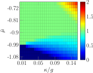
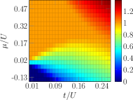
Figure 1: Mean density phase diagrams for (a) polaritons in the 1D JCH model and (b) bosons in the 1D BH model, in both cases for a system size $L=31$. Regions of constant mean density correspond to MI states.

The mean densities of either bosons or polaritons can be used to distinguish the two phases in both models, since the mean density is pinned to an integer in the MI regime, but not in the SF regime. Consequently, the locations of the phase boundary for our finite-size systems are quite clearly visible in Fig. 1. The shapes of the phase boundaries closely resemble the thermodynamic limit results of Refs. Kühner and Monien (1998); Rossini and Fazio (2007), though their positions are shifted slightly due to the finite-size system. Depicted is the region of the phase diagram where the $n=0$ and $n=1$ Mott lobes meet, as well as the low-density superfluid regions near the boundaries of these lobes. Roughly, the mean density of bosons (polaritons) increases with increasing $t$ ($\kappa$). This work is mainly concerned with the low-density superfluid regions of phase space, corresponding to low hopping and chemical potential.

The re-entrant shape of the $n=1$ Mott lobe can be clearly seen as the constant-density region of the BH model in Fig. 1, but is not as obvious in Fig. 1. At certain fixed values of $\mu$ within a continuous range, monotonically increasing the hopping parameter $t$ or $\kappa$ from zero causes the system to transition from the MI to the SF, back to the MI and again back to the SF regime Rossini and Fazio (2007). Viewed from within the Mott lobe, the lower part of the phase boundary (the hole boundary) is concave, while the upper part (the particle boundary) is convex. The particle and hole boundaries meet at a sharply cusped tip. The phase transition along the line of constant mean density passing through this point is in the $(d+1)$-dimensional XY universality class, which for $d=1$ is of the Berezinskii-Kosterlitz-Thouless (BKT) type Fisher et al. (1989); Kosterlitz and Thouless (1973) with Tomonaga-Luttinger parameter $K_{b}=1/2$ Kühner et al. (2000); Ejima et al. (2011). The MI-to-SF transition across either the particle or the hole boundary is generic (i.e. Gaussian like the condensation transition of an ideal Bose gas) and characterized by $K_{b}=1$ Kühner et al. (2000). This implies that the SF phase near the particle or hole boundaries should be characterized by one-particle correlation functions $G^{(1)}(r)\sim|r|^{-K_{b}/2}\sim 1/r^{1/2}$, consistent with the Tonks-Girardeau gas scaling.

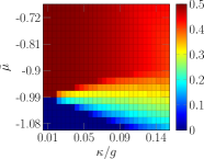
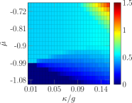
Figure 2: (a) Mean spin and (b) photonic excitation densities in the JCH model with $L=31$. These can vary throughout the MI phase.

In the JCH model, the mean densities of the spin and photonic species, depicted in Fig. 2, need not remain proportional to track each other. Consider first the mean spin excitation density, Fig. 2. In the atomic limit $\kappa=0$, the cavities are decoupled from each other and thus the overall ground state is the $L$-fold tensor product of the single-cavity lower-lying polariton states

$$|\psi_{\text{ground}}\rangle=\bigotimes_{i=1}^{L}|1-\rangle_{i}.$$ (18)

From Eqs. (3) and (5) in the case of zero-detuning, the single-cavity polariton ground states $|1-\rangle$ are equal-weight superpositions of a photonic and a spin excitation. Consequently, the mean spin excitation density is equal to $\frac{1}{2}$ in this limit. Conversely, in the hopping-dominated limit $\kappa\rightarrow\infty$, the photons and spins decouple. Each atom is then in the ground state so the mean spin excitation density vanishes. At intermediate $\kappa$ between these extremes, the data in Fig. 2 show that across the lower boundary of the Mott lobe (the hole boundary) there is a sharp drop in the mean density of spin excitations, which can be used to distinguish the two phases. By contrast, crossing the upper boundary, the mean spin excitation density varies smoothly from $\frac{1}{2}$ in the atomic limit to lower values, presumably tending towards $0$ in the limit $\kappa\rightarrow\infty$.

Next consider the mean photon density. Unlike the spin excitations, the number of photons and hence the mean photon density is unbounded from above in the grand canonical ensemble. In the large-hopping limit at fixed chemical potential, one expects the mean photon density to increase. In fact, for a lattice with coordination number $z_{c}$, an instability occurs when the hopping roughly satisfies $z_{c}\kappa/g>-\tilde{\mu}$; for larger values of the hopping, the ground state energy decreases without bound as a function of increasing photon number Koch and LeHur (2009). This regime is not considered in the calculations, as it corresponds to larger densities deep in the SF phase where fermionization is unlikely. The mean photon density within the $n=1$ MI lobe tracks with the mean spin excitation density in such a way that the overall polariton density is pinned to 1 per site, as expected. Crossing the upper (particle) boundary of the Mott lobe, the mean density of photons begins to increase rapidly with increasing hopping. This indicates that in the hopping-dominated limit, the system behaves like a photon superfluid, with the effects of the spins becoming negligible. On the other hand, in the intermediate regions between the $n=0$ and $n=1$ lobes, the mean photon density remains low; the reason is that at low hopping in one dimension, the effective repulsive interactions between photons become strong and thus there is an energy cost associated with adding photons to the system.

III.2 Correlation functions

III.2.1 One-body density matrix

Consider now the single-particle correlation function $G^{(1)}$, defined in Eq. (10). This has been calculated previously via DMRG for the 1D BH model, to verify the asymptotic predictions of the Luttinger liquid theory Pai et al. (1996), and to estimate the location of the critical value of $t/U$ for the BKT transition Kühner and Monien (1998). Similar plots of $G^{(1)}$ for varying interaction strengths in the $n=1$ MI lobe of the 1D BH model are shown in Ref. Ejima et al., 2012. The normalized version $C_{r}(s-r):=G^{(1)}(r,s)/\sqrt{N_{r}N_{s}}$ was also considered for the 1D BH model with an additional harmonic trapping potential Kollath et al. (2004) for various different sites $r$, and the coexistence of the two phases was found at certain points in the phase diagram.

As discussed in Sec. II.2, in the MI phase one expects this correlation function to decrease exponentially with distance, $G^{(1)}(r,s)\sim\exp(-|r-s|/\xi)$ over a correlation length $\xi$, while in the SF phase it should behave as a power law, $G^{(1)}(r,s)\sim 1/|r-s|^{\alpha}$ where $\alpha$ is some positive constant. The correlation functions are calculated for the JCH model (in which case $b\to a$ and $\sigma$ for photons and spins, respectively) and the BH model for systems of size $L=15$, 19, 23, 27, and 31. Consider for concreteness the shortest length $L=15$, for which the fits are the least reliable; the results are shown in Fig. 3. This size is chosen convey the worst-quality results for various system sizes. The correlations are measured with respect to the central site, in this case site number $8$. The point where $r=s$ is not plotted or used for the fit, since only the asymptotic form of the correlations for $|r-s|\gg 0$ is of interest. To mitigate boundary effects, the two sites closest to the (open) boundary of the system were also not considered. The correlations for the spins and the photons track each other very closely, so the results for photons are not presented.

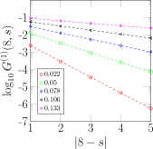
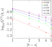
Figure 3: Representative plots of the correlation function $G^{(1)}(8,s)$ for the spin excitations in the JCH model with $L=15$. (a) $n=1$ MI phase at point $\tilde{\mu}=-0.900$, and (b) SF phase at point $\tilde{\mu}=-0.989$. In both cases the same five values of $\kappa/g$ are chosen with values given in the legends. The correlation functions are consistent with (a) exponentials and (b) power-laws.

The results indicate that the spin excitations and photons behave in close analogy to the bosons of the BH model; that is, the single-particle correlation functions are clearly exponential within the MI lobe and follow power laws in the SF regime. The power law relationship holds up well not only for $L=15$, but also for all larger values of $L$ considered. The exponent associated with the power law, corresponding to the slope of the log-log fit, is increasingly precise for larger values of $L$, with the standard error $\sim 1/\sqrt{L}$. The correlation function decreases most rapidly deep in the MI region but increasingly slowly as the phase boundary is approached. The results shown in Fig. 3 correspond to the SF phase at constant $\mu$, for values of $\kappa/g$ that range from almost immediately adjacent to the MI lobe ($\kappa/g=0.022$) almost to the edge of the phase diagram ($\kappa/g=0.133$) in Fig. 2. Unsurprisingly, the power-law fits are poor near the phase boundary (c.f. the points corresponding to $\kappa/g=0.022$) but improve as one moves further away.

The correlations exhibited by each type of carrier also track perfectly with each other. This result is in qualitative agreement with Ref. Knap et al. (2010), in which the same quantity was calculated using the Variational Cluster Approximation. In fact, this feature persists for all quantities discussed below, unless mentioned explicitly. An intriguing consequence of the identical behavior for the two species of excitations is that even though one normally views the atoms as mediating photonic interactions, one could just as well think of the photons as mediating atomic interactions; though the atoms are each isolated within their own cavities, they nevertheless feel each others’ presence.

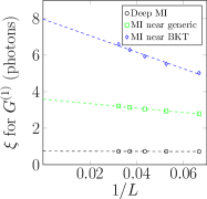
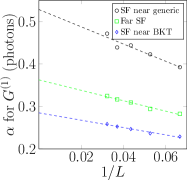
Figure 4: Representative finite-size scaling analysis of $G^{(1)}$ in the (a) MI and (b) SF regimes of the JCH model. The data points for the MI regime are $(\tilde{\mu},\kappa/g)=(-0.856,0.044)$ (deep within MI lobe), $(-0.856,0.128)$ (near generic transition), and $(-0.900,0.156)$ (near BKT point). The SF regime points are at $(-0.989,0.022)$ (near generic transition), $(-0.989,0.106)$ (deep within SF phase), and $(-0.989,0.156)$ (near BKT point).

The infinite-system values of the correlation length $\xi$ and the power $\alpha$ are estimated using a finite-size scaling analysis, as shown in Fig. 4 for a few representative points in phase space. The best exponential or power-law function is fit for $G^{(1)}$ for each value of $L=15$, 19, 23, 27, and 31, such as is shown in Fig. 3 for $L=15$. The values of $\xi$ and $\alpha$ are then plotted as a function of $1/L$, and the data are fit to a line whose intercept is interpreted as the corresponding value in the thermodynamic limit. The data are only weakly dependent on system size deep in the MI phase and near the generic phase boundary, but show a strong dependence near the BKT point. On the SF side the values of $\alpha$ are size-dependent for all three phase space points considered; this likely reflects the fact that along the $\tilde{\mu}=-0.989$ line the Mott boundary remains nearby. The same procedure is carried out for the BH model for comparison (not shown).

The phase diagram for the value of $\xi$ in the thermodynamic limit is displayed for the JCH and BH models in Fig. 5. Note however that one cannot obtain $\xi$ in this way immediately at the phase boundary. The true correlation length is expected to diverge, and a diverging correlation length cannot be accurately captured by a DMRG procedure with finite truncation $M$ Schollwöck (2011). Furthermore, the precise location of the phase boundary varies depending upon the size of the system, so a particular point in phase space near the boundary displayed for $L=31$ may or may not be in the Mott-insulating lobe, depending upon the system size. In Fig. 5, only the phase space points that are unambiguously within the $n=1$ lobe have been included; this accounts for the apparently smaller MI lobes than are depicted in Fig. 1.

The numerical results clearly indicate that the correlation length is independent of $\mu$ and is solely a function of $\kappa$ or $t$, smoothly increasing with increasing hopping. Since everywhere within the Mott lobe the state has a well-defined number of excitations $N_{\text{tot}}$, the only effect of varying the chemical potential by an amount $\Delta\mu$ while fixing $\kappa$ or $t$ is to shift the entire spectrum by an amount $N_{\rm tot}\Delta\mu$. The ground state itself at fixed hopping is therefore independent of $\mu$ within the lobe. The correlation function only increases as the BKT point is approached, not near the generic phase boundaries.

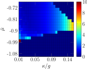
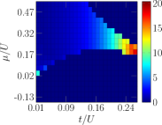
Figure 5: Phase diagrams for $\xi$ in the thermodynamic limit, assuming $G^{(1)}(r)\sim\exp(-r/\xi)$ in MI regime of the (a) JCH model (photons only) and the (b) BH model. The correlation length $\xi$ approaches the system size at the edge of the Mott lobe near the BKT point.

The value of $\alpha$ in the thermodynamic limit is calculated for all points in the superfluid phase for both the JCH and BH models, and the results are shown in Fig. 6. Right at the phase boundary, the exponent approaches values on the order of unity or higher. The same caveats mentioned above for the calculation of $\xi$ apply here as well. In addition, the spatial dependence of $G^{(1)}$ (an example of which is shown in Fig. 3) and the finite-size scaling data (an example of which is shown in Fig. 4) are much noisier right near the phase boundary.

Everywhere near the phase transition, however, the value of $\alpha$ is close to $0.5$. This value is consistent with what would be expected for a Tonks-Girardeau gas of photons [c.f. Eq. (17)] and matches the Luttinger parameter $K_{b}=1$, as discussed in Sec. III.1. In fact, $\alpha$ has previously been used to obtain the location of the phase boundary for the BH model, using infinite system DMRG with periodic boundary conditions Kühner and Monien (1998). This indicates that the low-density regime outside of the Mott lobes is in fact not strongly superfluid in nature. Rather, the results are consistent with the complete fermionization of the BH bosons and the JCH photons in the equivalent regime. Furthermore, since $G^{(1)}$ for the spin excitations and photons in the JCH model track each other so well (not shown), the spin excitations have also been fermionized, even though the atoms are treated as spins with no particular exchange statistics. The ‘SF’ designation of this phase therefore appears to be a misnomer, but it will be kept for clarity of exposition in what follows.

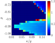
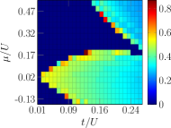
Figure 6: Phase diagrams for $\alpha$ in the thermodynamic limit, assuming $G^{(1)}(r)\sim r^{-\alpha}$ in SF regime of the (a) JCH model (photons only) and the (b) BH model. These values of $\alpha$ indicate strong fermionization of the photons in the JCH model.

The value of $\alpha$ decreases for increasing hopping $\kappa$ or $t$, but the trend is slow for the parameter range studied. By the edge of the plots in Fig. 6, the exponent for the SF phase between the $n=0$ and $n=1$ lobes has dropped to almost constant (in terms of $\mu$) values of $0.33$ and $0.29$ for the JCH and BH models, respectively. For larger values of $\mu$ where the density is higher the exponent drops off more rapidly, reaching a range of 0.081-0.254 for the JCH model and 0.226-0.336 for the BH model at the edge of the plots. These values are all quite different from the value $\alpha=0$ that one would expect for an ordinary superfluid, however.

III.2.2 Two-body correlation function

One of the most important signatures of fermionization within the low-density SF phase is found in the two-body correlation function $G^{(2)}(r,s)$ defined in Eq. (11) and its normalized variant $g^{(2)}(r,s)$ defined in Eq. (14), as discussed in Sec. II.3. Within the $n=1$ Mott-insulating lobe, one expects $g^{(2)}(r,s)=1-\delta_{r,s}$ irrespective of the model and the excitation, which is exactly what is observed. Of greater interest is the behavior of this correlation function in the SF regime for different mean densities. For a perfect superfluid the two-body correlation function is featureless, $g^{(2)}(r,s)=1$ in the bulk, reflecting the fact that all superfluid carriers occupy the same plane wave state. On the other hand, for a system of free fermions, the two-body correlation function exhibits two important features. The first is the presence of an exclusion hole at $r=s$ reflecting the Pauli exclusion principle. The second is the characteristic Friedel oscillations appearing on either side of the exclusion hole, with a wavelength $\lambda_{F}$ set by the mean density $n$ or Fermi wavelength $k_{F}$, as discussed in Sec. II.3.

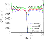
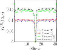
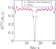
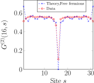
Figure 7: The spatial-dependence of the unnormalized two-body correlation function $G^{(2)}(16,s)$ for $L=31$ is shown for representative points in the SF phase where $\alpha\approx\frac{1}{2}$. Figures (a) and (b) correspond to photons at the points $(\tilde{\mu},\kappa/g)=(-0.989,0.039)$ and $(-0.989,0.106)$ in the JCH model, respectively; ‘T’ and ‘D’ in turn denote ‘theory’ and ‘data.’ Figures (c) and (d) correspond to bosons at the points $(\mu/U,t/U)=(0.019,0.066)$ and $(0.019,0.180)$, respectively.

The unnormalized two-body correlation functions $G^{(2)}(r,s)$ for the photons and spin excitations in the JCH model are plotted in Fig. 7 for representative points in the SF phase where $\alpha\approx\frac{1}{2}$; the BH results are also shown for comparison. (The momentum distribution $n(k)$ in the 1D BH model was previously considered for various interaction strengths within the $n=1$ MI lobe Ejima et al. (2011), and for both the MI and SF regimes at unit filling Kollath et al. (2004)). The data are compared with the analytical expression for free fermions at the same mean density, Eq. (15). The unnormalized two-body correlation function is plotted in order to make apparent the particle densities for the particular points in phase space. The two main signatures of fermionization in the SF phase, the exclusion hole and the Friedel oscillations, are evident in all the plots. At lower densities, the match between the data and the prediction based on non-interacting fermions is excellent. This indicates that the superfluid density at this point in the SF phase is close (if not exactly equal) to zero. One would expect the systems to behave more like a superfluid as the tunneling is increased and the excitation density increases, for points in phase space that are further from the phase boundary. Indeed this is the case; the data depicted in Figs. 7 and 7 show that the exclusion hole is now slightly filled in, and the Friedel oscillations are increasingly washed out.

An interesting feature in the case of the JCH model, not present in the BH model, is that the wavelength of the oscillations for both the photons and the bosons is set by the mean density of polaritons. The amplitude of $G^{(2)}$ for each carrier is determined by the density of just that carrier, however. More precisely, to obtain a fitting curve of the form of Eq. (15) for $G^{(2)}(r,s)$ for the photons (spin excitations), one must use the mean number of photons (spin excitations) as the value of $N$ in the prefactor $\left(N/(L+1)\right)^{2}$, but the number of polaritons in the oscillatory functions appearing in $A(r,s)$ and $B(r,s)$. Hence, the spin excitations and the photons are individually fermionized, inasmuch as they have inherited this property from the polaritons.

III.3 Other measures of the ground state

III.3.1 Superfluid fraction

The most compelling evidence for the existence of a SF phase would be the presence of a non-zero superfluid order parameter. An example of such an order parameter is the superfluid fraction or superfluid stiffness $f_{s}$, the ratio of particles exhibiting superfluid flow to the total number of particles. The factor $f_{s}$ can be calculated numerically by imposing periodic boundary conditions and applying a phase twist $\Theta\ll\pi$ to the boundary conditions Fisher et al. (1973); Krauth (1991); Singh and Rokhsar (1994); Roth and Burnett (2003a). In practise, this can be accomplished by means of a Peierls factor applied to the bosonic creation and annihilation operators in the BH and JCH models, which has the effect of modifying the hopping terms via $a_{i}^{\dagger}a_{j}\longmapsto a_{i}^{\dagger}a_{j}e^{-\mathrm{i}\Theta/L}$ Roth and Burnett (2003b). While this induces a velocity $v=(2J)\nabla\Theta$ for each quantum particle ($J$ is the hopping coefficient corresponding to $\kappa$ in the JCH model or $t$ in the BH model) because the current density is $j=nv$, only the particles in the superfluid will respond collectively. As a result, the ground state energy will increase relative to the twist-free case solely due to the kinetic energy of the superfluid particles. From this change of the ground state energy, the superfluid fraction can be determined:

$$f_{s}=\frac{L}{2Jn}\left.\frac{\partial^{2}E_{0}(\Theta)}{\partial\Theta^{2}}\right|_{\Theta=0}\approx\frac{L}{Jn}\frac{E_{0}(\Theta)-E_{0}}{\Theta^{2}},$$ (19)

where $E_{0}$ is the ground state energy with no phase twist and $E_{0}(\Theta)$ is ground state energy with overall twist $\Theta\ll\pi$. The latter expression is a finite-difference approximation for the second derivative of the energy with respect to the phase twist, using the central three-point stencil. This calculation of $\rho_{s}$ has previously been performed at constant density near the BKT transition of the 1D BH model across the tip of the $n=1$ Mott lobe Pai et al. (1996); a significant jump in $\rho_{s}$ across the transition was found in that work. This work instead examines $\rho_{s}$ at representative points in the low-density SF phase far from the transition, with considerably different results.

In the numerical calculations, we considered various points in the SF phase using five different finite-size systems $L=15,19,23,27,31$. Periodic boundary conditions are required, which are computationally more demanding for the DMRG method than are open boundary conditions (see the discussion in Sec. II.4); hence, only a set of representative points in the SF phase were considered. Recall from Sec. II.4 that the $n=1$ BKT points in the JCH and BH models are located at approximately $(\tilde{\mu},\kappa/g)=(-0.95,0.2)$ Rossini and Fazio (2007); Mering et al. (2009) and $(\mu/U,t/U)=(0.09,0.3)$ Kühner and Monien (1998); Kühner et al. (2000); Ejima et al. (2011), respectively. We therefore considered these three points in the SF phase of the JCH model: $(-0.944,0.133)$, $(-0.989,0,028)$, and $(-1.00,0.240)$. The first is just left of the BKT point, in the vicinity of the hole boundary, the second is between the $n=0$ and $n=1$ Mott lobes, and the third is to the right of the BKT point. In particular, the first two points correspond to mean polariton densities $n<1$, while the third has $n>1$. For the BH model we considered the two points: $(0,0.08)$ and $(0,0.5)$; again, the first is left of the BKT point in the vicinity of the hole boundary, while the second point is much to the right, in the deep SF phase well beyond the region depicted in Figs. 1 and 6. The first of these points has mean boson density $n<1$ and the second, $n>1$.

The ground-state energy was obtained for these points in the SF region, for phases $\Theta/\pi\in(0.0,1.0)$ in increments of $0.2$. Note that the ground state energy is invariant under the transformation $\Theta\longmapsto-\Theta$. For each value of $L$, the second derivative in Eq. (19) was then calculated using $\Theta=0.2\pi$. The results were then verified by estimating the derivative using a central-difference approximation with five-point ($\Theta/\pi\in\left\{0,\pm 0.2,\pm 0.4\right\}$) and seven-point stencils ($\Theta/\pi\in\left\{0,\pm 0.2,\pm 0.4,\pm 0.6\right\}$); no discernible difference from the method of Eq. (19) was observed in the results so obtained. The values of $f_{s}$ were also obtained by extracting the coefficient for the quadratic term in a polynomial fit of $E_{0}(\Theta)$. Again, no discernible differences from the central-difference results were found using this approach. Once the value of $f_{s}$ was obtained for a given system size, a finite-size scaling analysis in $1/L$ was performed to interpolate to the thermodynamic limit. As a final check on the results, the calculation in Eq. (19) was repeated with smaller values of the phase twist, $\Theta/\pi\in[0.0,0.2]$ in increments of $0.02$. For $\Theta/\pi<0.06\pi$, the values of $\rho_{s}(L)$ could not be reliably fitted to determine the value in the thermodynamic limit (the problem of dividing one small number by another). However, for $\Theta/\pi\geq 0.06$, the results were consistent with those obtained with $\Theta/\pi=0.2$.

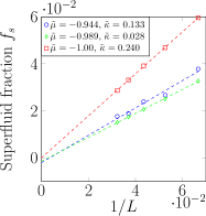
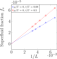
Figure 8: Superfluid fraction for the (a) JCH and (b) BH model outside but near the $n=1$ MI lobe. For the JCH model, the symbol $\tilde{\kappa}=\kappa/g$ is used for compactness. For both systems, the curve marked by red squares (color online) is beyond the critical hopping value for the BKT transition for the $n=1$ MI lobe, while the others are not. In both cases, the superfluid fraction $f_{s}$ tends to 0 in the thermodynamic limit.

BH model				JCH model
$\mu/U$	$t/U$	$f_{s}$	$\Delta f_{s}$	$\tilde{\mu}$	$\kappa/g$	$f_{s}$	$\Delta f_{s}$
0	0.08	0.0007	0.0008	-0.944	0.133	-0.0020	0.0025
0	0.5	-0.0001	0.0001	-0.989	0.028	-0.0014	0.0004
				-1.00	0.240	0.0000	0.0004

Table 1: Numerical values (with uncertainties) of superfluid fraction $f_{s}$ in thermodynamic limit, for phase space points indicated in Fig. 8.

The finite-size scaling results for the superfluid fraction $f_{s}$ are shown in Fig. 8, and the resulting values and uncertainties of $f_{s}$ in the thermodynamic limit are displayed in Table 1. These values are determined by the standard least-squares minimization procedure for linear fitting. In all cases, except for the JCH point marked by red squares in Fig. 8, the obtained thermodynamic limit value of the superfluid density contains 0 within its error interval. For the one exceptional case, the thermodynamic limit $f_{s}$ is an order of magnitude smaller than the finite-size values (as well as unphysically negative), indicating that the superfluid fraction should vanish in the thermodynamic limit. It is interesting to note that the finite-size scaling plot for the BH point $(\mu/U,t/U)=(0.5,0.5)$ (not shown), which is situated above the particle boundary of the $n=1$ lobe, is identical to the scaling of the $(0.0,0.5)$ point shown in Fig. 8. Similar behavior is found in the JCH model in the SF region to the right of the BKT point. Consider for example the point $(\tilde{\mu},\kappa/g)=(-0.750,0.240)$ located above the $(-1.000,0.240)$ point in Table 1. The infinite-system superfluid fraction inferred from finite-size scaling is $f_{s}=0.0006\pm 0.0033$, consistent with zero. This indicates that the superfluid density is only weakly dependent on the chemical potential for a given hopping strength. The data strongly suggest that the superfluid density is zero throughout the low-density SF region studied.

III.3.2 Condensate fraction

The condensate fraction $f_{c}$ is defined as the proportion of particles in the lowest-lying single-particle eigenstate of the system. In practice, this can be obtained by the largest eigenvalue of the single-particle density matrix $G^{(1)}(r,r^{\prime})$ Penrose and Onsager (1956); Penrose (1951). In fact the entire spectrum, known as the entanglement spectrum Li and Haldane (2008), can be used to identify quantum phases. In the atomic limit, the single-particle ground state for a system of length $L$ is $L$-fold degenerate, since there is no preferred lattice site. In the non-interacting limit, the finite-size systems have a sinusoidal single-particle ground state. At zero temperature, one expects macroscopic occupation of the ground state in the SF regime, tending towards unit occupation for large $J/U$. In the MI regime one expects the particles to be distributed evenly across many nearly-degenerate single particle states, a phenomenon known as fragmentation for large occupation of a single site Spekkens and Sipe (1999); Mueller et al. (2006). If the particles have fermionized, however, then no such macroscopic occupation should occur; $f_{c}$ can therefore be viewed as another signature of fermionization.

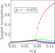
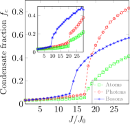
Figure 9: Maximal eigenvalues of the reduced single-particle density matrix for $L=31$. In (a), the five largest eigenvalues of the photon density matrix are shown for fixed $\tilde{\mu}=-0.678$ as a function of hopping amplitude $\kappa/g$. In (b), the largest eigenvalue of the density matrix (identified with the condensate fraction $f_{c}$ in the SF phase) for spin excitations and photons in the JCH model, and for bosons in the BH model, are shown as a function of generalized hopping $J/J_{0}$ at fixed chemical potential $\tilde{\mu}=-0.678$ and $\mu/U=0.55$, respectively. The inset shows the lower density case $\tilde{\mu}=-0.922$ and $\mu/U=0.133$ for comparison.

The five largest eigenvalues of the single-particle photon density matrix are plotted in Fig. 9(a) in the JCH model for $\tilde{\mu}=-0.678$ and $L=31$ as a function of hopping strength $\kappa/g$. This corresponds to the constant $\tilde{\mu}$ line near the very top of Fig. 1(a). In the zero-hopping limit $\kappa/g\to 0$, each photon is perfectly localized to each site, and the eigenvalues are precisely $1/L$ (note that the density matrix is normalized to unity rather than the total number of particles). As $\kappa/g$ increases the degeneracy is broken and the largest eigenvalues increase due to the fluctuations of the site occupations, while others decrease to preserve the normalization (not shown). At a critical hopping strength $\kappa/g\approx 0.085$ coinciding with the superfluid transition at this value of $\tilde{\mu}$, one of the eigenvalues increases precipitously relative to the others, signifying the macroscopic occupation of a single mode. This eigenvalue is associated with the (quasi)condensate fraction. For larger hopping strengths the condensate fraction tends towards unity, as expected for a non-interacting Bose gas at zero temperature.

Fig. 9(b) compares the values of the condensate fraction for the BH bosons with the JCH photons and spins along the same line of constant chemical potential considered above, corresponding to $\mu/U=0.55$ in the BH model (recall that $\mu/U\sim 1.707(\tilde{\mu}+1)$ as discussed in Sec. II.2). The value of $f_{c}$ for each model is plotted for fixed size $L=31$ as a function of the hopping $J$, where $J=\kappa$ ($t$) in the JCH (BH) case, in units of the minimum hopping considered $J_{0}$ corresponding to $\kappa_{0}/g=0.00556$ and $t_{0}/U=1.7\kappa/g=0.00948$. Though the onset of superfluidity occurs for smaller $J/J_{0}$ in the BH case, consistent with Fig. 1, the condensate fraction does not increase as quickly as that of the photons in the JCH case. This might simply reflect the fact that the mean carrier density is lower for the BH model at the top right point in the phase diagram than for the JCH model, which would discourage condensation. At lower mean particle densities on the SF side $\tilde{\mu}=-0.922$ ($\mu/U=0.133$), shown in the inset of Fig. 9(b), the $f_{c}$ for the BH case is larger than that for the photons of the JCH model, but neither reach 50%. The finite-size results suggest that $f_{c}$ tracks the mean particle density, as is discussed further below.

Interestingly, the spin excitations in the JCH model also show strong evidence of condensation. The value of $f_{c}$ on the SF side reaches approximately half that for the photons for the largest value of $J/J_{0}$ considered for this value of $\tilde{\mu}$. For lower values of $\tilde{\mu}$ in the vicinity of the $n=0$ Mott lobe, the ratio of $f_{c}$ for spin excitations to photons approaches unity (not shown). These results are generally consistent with observations above that indicate that the spin and photon degrees of freedom follow each other closely. The condensation in the spin sector therefore appears to be driven sympathetically by the photons via the polariton excitations. The results are nevertheless somewhat surprising, suggesting that the spin excitations are delocalized.

To obtain the condensate fraction in the thermodynamic limit, the values of $f_{c}$ were obtained throughout the phase diagram for each triple $(\mu,J,L)$, where $L=15,19,23,27,31$ using DMRG subject to open boundary conditions. The finite-size scaling analysis was performed for the SF regime only because the procedure is not robust for the points in the MI regime. Nevertheless, the finite-size results within the MI regime clearly indicate fragmentation, and since the macroscopic degeneracy in the atomic limit is true independent of system size, there is no reason to believe that the results in the thermodynamic limit would be qualitatively different.

The condensate fractions for JCH and BH models in the thermodynamic limit throughout the explored SF regime of the phase diagram are shown in Fig. 10(a) and (b), with the MI lobes explicitly zeroed out. Both pictures have the same color scale and are plotted with the axes corresponding to equivalent energy scales. The results are qualitatively similar for both models, but there are some quantitative differences. The value of $f_{c}$ rises more rapidly with increasing hopping in the JCH model than in the BH model, attaining $f_{c}=0.800$ at the highest mean densities investigated, as opposed to only $f_{c}=0.500$ for the BH model. The values of $f_{c}$ shown in the phase diagrams strongly resemble the mean densities of spins, photons, and bosons, such shown in Fig. 1. Deep in the SF regime the $f_{c}$ closely follow the mean excitation densities, suggesting that the proclivity toward condensation is governed by the mean density. That said, as the Mott lobe boundary approaches the ratios of $f_{c}$ to the respective mean densities is found to increase markedly even as $f_{c}$ approaches zero.

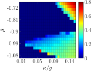
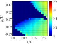
Figure 10: Condensate fraction for the (a) JCH model (photons only) and the (b) BH model outside but near $n=1$ MI lobe, in the thermodynamic limit. In both cases, the condensate fraction within the MI lobes is zeroed out.

While there need be no direct relationship between Bose-Einstein condensation and superfluidity, it is nevertheless somewhat surprising that the condensate fraction in the thermodynamic limit would be so large throughout the SF region where the superfluid fraction remains zero. These results are nevertheless consistent with the small values of $\alpha$ in the SF region, shown in Fig. 6 (recall that $\alpha\to 0$ for Bose-Einstein condensates), as well as with the filling in of the exclusion hole and the disappearance of the Friedel oscillations found in the spatial-dependence of the two-body correlation function (c.f. Fig. 7). In addition, the value of $f_{c}$ is consistently small in the low-density SF regime, as expected for a fermionized gas.

III.3.3 Entanglement properties

Much can be learned about the ground states of physical systems by examining the properties of subsystems. A notable example is the entropy of entanglement Nielsen and Chuang (2000). This is obtained by partitioning the system into a block of contiguous lattice sites $b\subset\mathcal{L}$, where $\mathcal{L}$ denotes the full lattice, and its complement $b^{\prime}$. The entropy of entanglement associated with this bipartition is given by

$$S_{\rho_{b}}=-\text{Tr}(\rho_{b}\text{ln}\rho_{b}),$$ (20)

where $\rho_{b}$ is the reduced density matrix of the state over $b$. Analytical formulas for the entanglement entropy of non-interacting fermions and bosons on a lattice exist for the semi-infinite chain Peschel and Eisler (2009) but we are not aware of any for finite-size systems greater than a few sites.

The scaling of the entanglement entropy with the size of the subsystem is intimately linked with the utility of DMRG as a simulation method. For a wide array of physical systems, the entanglement entropy obeys an area law Eisert et al. (2010), meaning that the entanglement entropy $S_{\rho}$ associated with $\rho_{b}$ is proportional to the number of sites at the interface between $b$ and $b^{\prime}$ (henceforth denoted $l$), rather than to its volume or cardinality. In one dimension, the area law corresponds to a value of $S_{\rho}$ that saturates for some finite value of $l$:

$$S_{\rho}(l)\leq D,$$ (21)

where $D$ is a constant, independent of $l$ (of course $l=2$ is itself constant). Only states satisfying Eq. (21) can be efficiently simulated by DMRG for large system sizes, because the variational ansatz used by the DMRG algorithm explicitly assumes that the area law is satisfied Vidal (2003); Eisert et al. (2010). Asymptotic scaling results Wolf (2006) reveal that free fermions always logarithmically violate the area law in any dimension in both the continuum and on a lattice, whereas free bosons in 1D satisfy the area law away from criticality Plenio et al. (2005).

The entanglement entropy associated with a finite block can be used to distinguish bosonic and fermionic behavior. The entanglement entropy of the 1D non-interacting Bose gas is a smooth function, whereas that for the non-interacting Fermi gas oscillates with $l$. This is because at zero temperature the bosons condense into the smooth lowest-lying eigenstate of the hopping model, while the Pauli exclusion principle forces fermions into oscillatory excited states. Generally, the entanglement entropy for bosons is larger than for fermions because the number of accessible states $\Omega_{b}$ is exponentially greater than $\Omega_{f}$, meaning that when the system is bipartitioned, for each configuration of the left half of the chain there are an exponentially larger number of compatible configurations for the right half in the bosonic case.

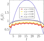
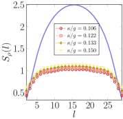
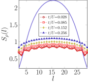
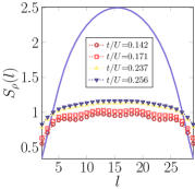
Figure 11: The photon and boson entanglement entropy $S_{\rho}(l)$ for a contiguous block of sites of length $l=3$ to 29 with $L=31$, for the JCH and BH models, respectively. Two mean densities are considered, $n=0.645$ for the (a) JCH and (c) BH models, and $n=1.129$ for the (b) JCH and (d) BH models. The solid blue line is the exact value of $S_{\rho}^{b}$ for an ideal lattice Bose gas, and the solid red line in (a) and (c) is the corresponding value $S_{\rho}^{f}$ for the ideal Fermi gas.

The entanglement entropy $S_{\rho}(l)$ is plotted in Fig. 11 as a function of $l$ for $3\leq l\leq 29$ ($L=31$) along a contour of constant density in the SF regime. The results are displayed for both the JCH and BH models at two different mean densities: $n=0.645$ and $n=1.129$. The corresponding entropy profiles for the free Bose and Fermi gases at the same mean density, calculated numerically, are plotted for comparison. The bosonic entanglement entropy increases approximately linearly with $l$ for $l\ll L$. The fermionic entanglement entropy displays strong oscillations but much weaker $l$-dependence. At the lower mean density considered, the photon entanglement entropy profile is very similar to the ideal Fermi gas for small hopping, again providing strong evidence for fermionization. As the hopping increases, the oscillations become less pronounced and the value of the entropy increases; presumably the entropy profile would converge to that of the ideal Bose gas for very large hopping amplitudes. For the $n>1$ case, which precludes fermionization in this single-band model, the oscillations are almost completely washed out. The magnitude of entanglement entropy remains well below the ideal Bose gas limit, however.

While the entanglement entropy can be used to help distinguish quantum phases, it does not directly quantify the possible use of this entanglement for quantum computation. Indeed, it is difficult to conceive of how one could encode quantum algorithms into the (generally delocalized) indistinguishable bosons of the BH model. The JCH model, on the other hand, has distinguishable quantum registers in the spin states of the two-level atoms (i.e. qubits) which are each localized to a different optical cavity. If entanglement were generated between cavity atoms by the itinerant photons, then the coupled cavity QED could potentially be a natural environment for quantum computation.

It was recently proven that universal quantum computation is possible as long as the entanglement associated with arbitrary bipartitions is non-vanishing Van den Nest (2013). One useful measure that is closely related to the entanglement entropy is the localizable entanglement Verstraete et al. (2004a, b); Popp et al. (2005). The localizable entanglement $E^{\text{LE}}_{ij}$ between qubits $i$ and $j$ of a multiqubit system is defined as the maximal entanglement that can be concentrated between qubits $i$ and $j$ via local (i.e. single-spin) operations and classical communication, and is a non-negative number in the range $\left[0,1\right]$. In a spin network, the localizable entanglement is lower-bounded by the maximal absolute value of the spin-spin correlation function $C^{\alpha,\beta}_{ij}:=\langle\sigma^{\alpha}_{i}\sigma^{\beta}_{j}\rangle-\langle\sigma^{\alpha}_{i}\rangle\langle\sigma^{\beta}_{j}\rangle$ over all possible axes $\alpha,\beta\in\mathbb{R}^{3}$ Popp et al. (2005); Amico et al. (2008). Using $\sigma^{z}_{i}=\sigma^{+}_{i}\sigma^{-}_{i}-I/2=n_{i}^{\rm spin}-I/2$ where $I$ is the $2\times 2$ identity matrix, and if $\alpha=\beta=z$, the localizable entanglement is at least as large as

$$\left|C^{zz}_{ij}\right| \equiv\left|\langle N_{i}N_{j}\rangle-\langle N_{i}\rangle\langle N_{j}\rangle\right|,$$

where here $N_{k}=\sigma^{+}_{k}\sigma^{-}_{k}$ is the local spin excitation number operator, satisfying $0\leq\langle N_{k}\rangle\leq 1$. The localizable entanglement is therefore closely related to the (unnormalized) two-body correlation function, defined in Eq. (11). For $i\neq j$ (the only case of interest for entanglement), one obtains $C^{zz}_{ij}=G^{(2)}(i,j)-\langle N_{i}\rangle\langle N_{j}\rangle\approx G^{(2)}(i,j)-n^{2}$ (the local excitation number is approximately equal to the mean density – the total number of excitations over all sites – if the density is almost constant).

The behavior of the spin-spin correlation function in the thermodynamic limit can be estimated under the assumption that the spin excitations have completely fermionized, using Eq. (14) for a ring geometry or Eqs. (15-16) for open boundary conditions. Consider the symmetric pair of sites $i_{\mp}=(L\mp a)/2$, separated by $a$. Using either geometry one obtains $G^{(2)}(i_{-},i_{+})\rightarrow n^{2}\left[1-\sin^{2}(\pi na)/(\pi na)^{2}\right]$, assuming short-ranged correlations in the bulk where $a$ remains constant as $L$ increases; for small $n$, the spin-spin correlation function approaches $-n^{2}$. If the separation instead scales like $a\sim L$, then $G^{(2)}(i_{-},i_{+})\rightarrow n^{2}$ and $C^{zz}_{i_{-}i_{+}}\rightarrow 0$.

The correlation function $C^{zz}_{ij}$ was calculated throughout the phase region investigated. Restricting $i$ and $j$ to lie between $\lceil L/4\rceil$ and $\lceil 3L/4\rceil$ to avoid boundary effects, $\left|C^{zz}_{i,j}\right|$ take the largest values when $|i-j|=1$ ($i=j$ is explicitly excluded). The values of $C^{zz}_{i,i\pm 1}$ were found to be close to zero everywhere in the MI phase, consistent with the strong density localization and small density fluctuations which are the hallmark of MI states. Likewise, the values of $C^{zz}_{i,i\pm 1}$ tend to zero for all $i$ at high mean densities and hopping where the BEC fraction is large. This reflects the smooth and relatively constant profile of the two-body correlation function other than the remnant of the exclusion hole at short distances, as shown in Fig. 7.

At low density and hopping amplitude in the SF regime, the magnitudes of $C^{zz}_{i,i\pm 1}$ generally range between $0.02$ to $0.05$. This is a direct consequence of the large exclusion hole in the spin density-density correlation function in the vicinity of $i\sim j$, inherited from the strongly fermionized polaritons. The spin-spin correlation function reaches a maximum value in the region directly adjacent to the hole boundary of the $n=1$ Mott lobe. At the point $(\tilde{\mu},\kappa/g)=(-0.989,0.0167)$ where the mean spin excitation density is $n=0.3825$, the numerics yield $\left|C^{zz}_{i,i\pm 1}\right|=0.075$. The fermionized theory predicts the comparable but slightly larger value of $\sin^{2}(\pi n)/\pi^{2}\approx 0.088$. The difference between theory and computation is likely partly due to the fact that the spin excitations have not perfectly fermionized.

Because we have only considered the $zz$ quadrature of the spin-spin correlation function, the numerical value is a lower-bound to the lower-bound of the localizable entanglement. The actual value of the localizable entanglement in the Tonks-Girardeau regime could well be larger. In any case, the numerical results suggest that there is sufficient entanglement between the atoms in the ground state of coupled cavities to support universal quantum computation, if a suitable strategy to embed this environment in a quantum circuit could be found.

IV Conclusions

In this work, we have explored the Mott-Insulator to superfluid transition of the one-dimensional Jaynes-Cummings-Hubbard (JCH) model in the strong-coupling regime with no detuning. The purpose of the work has been two-fold. First and foremost, it has been to study the nature of the ground state in the vicinity of the phase transition, in particular to demonstrate that the photons are in fact strongly fermionized in the low-density ‘superfluid’ phase. Second, it has been to compare and contrast the properties of the ground state to that of the 1D Bose-Hubbard (BH) model, in order to highlight the unique features of the JCH model. The results were obtained by finding the ground state using the finite-system Density Matrix Renormalization Group, computing various static properties, and then performing a finite-size scaling analysis to infer the thermodynamic limit.

The main result is that in one dimension, the ground state of the JCH model in the low-density regime outside the Mott-insulating lobes is dramatically different from that of a conventional superfluid. Rather, the system in the region widely characterized as a superfluid (SF) is in fact a Tonks-Girardeau gas of strongly fermionized excitations, much as occurs in the one-dimensional BH model. This is evidenced by the power law of the single-particle density matrix in both the spin and photonic sectors of the model, by the Friedel oscillations and the fermionic exclusion hole in the two-body density matrix for each sector, and by the strongly fermionic profile of the entanglement entropy. Thus coupled cavity QED provides a natural and accessible environment for the realization of strongly correlated photons. The photon fermionization should be readily observable in experiments using standard photon correlation spectroscopy Carmichael et al. (1996).

We have calculated the superfluid fraction for both species of excitation in the JCH model, both within the low-density SF regime as well as for large tunneling beyond the expected BKT transition point, and found that the superfluid density vanishes in the thermodynamic limit in both cases. At the same time, we have found that the Bose-Einstein condensate fraction for the photons and spin excitations is non-vanishing throughout the SF region. The value of the condensate fraction is low at very low densities, consistent with fermionization, but can reach as high as 80% at high densities for the photons. This indicates the existence of a (quasi)condensate of photons and even spin excitations, despite the absence of superfluidity.

The same static properties for the 1D BH model have been calculated in an equivalent parameter regime in phase space, and the results have been compared in detail to those obtained within the JCH model. Broadly, the behavior of the two models coincide: neither exhibits a true Mott-insulator to conventional superfluid transition. However, various quantitative differences exist. The single-particle correlations in the JCH ground state within the $n=1$ Mott lobe decay more rapidly with increasing hopping that in the BH case, while those in the intermediate region between the $n=0$ and $n=1$ lobes decay more slowly. Consistently with this result, the condensate fraction for the JCH photons rises more rapidly with increasing hopping than for the BH bosons. While a formal mapping between the BH and JCH models does not exist, the results indicate that the well-known manifestations of the BH model will be largely reproduced in physical systems that are well-described by the JCH model.

That said, the JCH model has some intriguing features not shared by the BH model, owing to the presence of two species. The spin and photon degrees of freedom are inextricably linked through the fundamental polariton excitations. Thus Bose-Einstein condensation of photons implies that the spin excitations are similarly condensed. The atomic spin states are thereby effectively delocalized across the entire system in spite of the fact that each atom is confined to its respective cavity. This observation opens the intriguing possibility of inducing spin liquid-like states in cavity QED systems. In fact, the possibility of spin dimerization in the JCH model with large positive detuning $\delta\gg 0$ (which induces frustration and is not considered in the present work) has been noted very recently Zhu et al. (2013). Likewise, atoms in different cavities are spontaneously entangled via the itinerant photons, as evidenced by the non-zero value of the localizable spin entanglement in the SF regime. It would be intriguing to systematically consider the effect of non-zero detuning on the properties of the ground states, but this is beyond the scope of the present work.

The majority of the parameter space explored in this project is in the vicinity of a phase transition, but the convergence of the DMRG algorithm is not guaranteed very close to the phase boundary. It could be fruitful to compare the results with those obtained using a method such as Multiscale Entanglement Renormalization Ansatz Vidal (2008), which is specifically tailored to work well with critical systems. In a similar vein, the calculations (in particular the superfluid density) could be repeated with a method that is designed for handling infinite systems directly, such as iDMRG McCulloch (2008); Crosswhite et al. (2008). This would avoid the need to perform finite-size scaling on small systems to make quantitive statements about the thermodynamic limit.

Cavity quantum electrodynamics is a promising candidate for quantum information processing applications, since the local atoms can be used as qubits and the photons can be used to generate entanglement between them. Our results suggest that the localizable entanglement is always finite throughout the SF region. It would be interesting to determine if the ground state for a more complex network of coupled cavities could be a resource for measurement-based quantum computation, where universal quantum algorithms are effected solely via single-qubit measurements conditioned on previous outcomes Briegel et al. (2009). Preliminary calculations indicate that the type of correlations between atoms in the current 1D JCH model with zero detuning are probably not suitable for gate teleportation via measurements. This will be explored more fully in future work.

V Acknowledgements

The authors are grateful for research funding from the Natural Sciences and Engineering Research Council of Canada, Alberta Innovates – Technology Futures, and the Canadian Institute for Advanced Research. This research has been enabled by the use of the ALPS software package, particularly the dmrg application, as well as by computing resources provided by WestGrid and Compute/Calcul Canada.

References

- Fisher et al. (1989) M. P. A. Fisher, P. B. Weichman, G. Grinstein, and D. S. Fisher, Phys. Rev. B 40, 546 (1989).
- van der Zant et al. (1992) H. S. J. van der Zant, F. C. Fritschy, W. J. Elion, L. J. Geerligs, and J. E. Mooij, Phys. Rev. Lett. 69, 2971 (1992).
- Bloch (2005) I. Bloch, Nat. Phys. 1, 23 (2005).
- Corrielli et al. (2013) G. Corrielli, A. Crespi, G. D. Valle, S. Longhi, and R. Osellame, Nat. Commun. 4, 1555 (2013).
- Hartmann et al. (2006) M. J. Hartmann, F. G. S. L. Brandão, and M. B. Plenio, Nat. Phys. 2, 849 (2006).
- Greentree et al. (2006) A. D. Greentree, C. Tahan, J. H. Cole, and L. C. L. Hollenberg, Nat. Phys. 2, 856 (2006).
- Angelakis et al. (2007) D. G. Angelakis, M. F. Santos, and S. Bose, Phys. Rev. A 76, 031805 (2007).
- Houck et al. (2012) A. A. Houck, H. E. Türeci, and J. Koch, Nat. Phys. 8, 292 (2012).
- Mott and Peierls (1937) N. F. Mott and R. Peierls, Proc. Phys. Soc. 49, 72 (1937).
- Mott (1949) N. F. Mott, Proc. Phys. Soc. A 62, 416 (1949).
- Mott (1982) N. F. Mott, Proc. Roy. Soc. London. A. 382, 1 (1982).
- Kapitza (1938) P. Kapitza, Nature 141, 74 (1938).
- Allen and Misener (1938) J. F. Allen and A. D. Misener, Nature 141, 75 (1938).
- Landau (1941) L. D. Landau, J. Phys. USSR 5, 71 (1941).
- Greiner et al. (2002) M. Greiner, O. Mandel, T. Esslinger, T. W. Hänsch, and I. Bloch, Nature 415, 39 (2002).
- Stöferle et al. (2004) T. Stöferle, H. Moritz, C. Schori, M. Köhl, and T. Esslinger, Phys. Rev. Lett. 92, 130403 (2004).
- Spielman et al. (2007) I. B. Spielman, W. D. Phillips, and J. V. Porto, Phys. Rev. Lett. 98, 080404 (2007).
- Gemelke et al. (2009) N. Gemelke, X. Zhang, C.-L. Hung, and C. Chin, Nature 460, 995 (2009).
- Bakr et al. (2010) W. S. Bakr, A. Peng, M. E. Tai, R. Ma, J. Simon, J. I. Gillen, S. Foelling, L. Pollet, and M. Greiner, Science 329, 547 (2010).
- Haller et al. (2010) E. Haller, R. Hart, M. J. Mark, J. G. Danzl, L. Reichsoellner, M. Gustavsson, M. Dalmonte, G. Pupillo, and H.-C. Naegerl, Nature 466, 597 (2010).
- Trotzky et al. (2010) S. Trotzky, L. Pollet, F. Gerbier, U. Schnorrberger, I. Bloch, N. V. Prokof’ev, B. Svistunov, and M. Troyer, Nat. Phys. 6, 998 (2010).
- Hartmann et al. (2007) M. J. Hartmann, F. G. S. L. Brandao, and M. B. Plenio, Phys. Rev. Lett. 99, 160501 (2007).
- Rossini and Fazio (2007) D. Rossini and R. Fazio, Phys. Rev. Lett. 99, 186401 (2007).
- Carusotto et al. (2009) I. Carusotto, D. Gerace, H. E. Tureci, S. De Liberato, C. Ciuti, and A. Imamoǧlu, Phys. Rev. Lett. 103, 033601 (2009).
- Kiffner and Hartmann (2010) M. Kiffner and M. J. Hartmann, Phys. Rev. A 81, 021806 (2010).
- Halu et al. (2013) A. Halu, S. Garnerone, A. Vezzani, and G. Bianconi, Phys. Rev. E 87, 022104 (2013).
- Hayward et al. (2012) A. L. C. Hayward, A. M. Martin, and A. D. Greentree, Phys. Rev. Lett. 108, 223602 (2012).
- Schiró et al. (2012) M. Schiró, M. Bordyuh, B. Öztop, and H. E. Türeci, Phys. Rev. Lett. 109, 053601 (2012).
- Hartmann et al. (2008) M. J. Hartmann, F. G. S. L. Brandão, and M. B. Plenio, New J. Phys. 10, 033011 (2008).
- Makin et al. (2008) M. I. Makin, J. H. Cole, C. Tahan, L. C. L. Hollenberg, and A. D. Greentree, Phys. Rev. A 77, 053819 (2008).
- Jaynes and Cummings (1963) E. Jaynes and F. Cummings, Proc. IEEE 51, 89 (1963).
- Birnbaum et al. (2005) K. Birnbaum, A. Boca, R. Miller, A. Boozer, T. Northup, and H. Kimble, Nature 436, 87 (2005).
- Aichhorn et al. (2008) M. Aichhorn, M. Hohenadler, C. Tahan, and P. B. Littlewood, Phys. Rev. Lett. 100, 216401 (2008).
- Koch and LeHur (2009) J. Koch and K. LeHur, Phys. Rev. A 80, 023811 (2009).
- Schmidt and Blatter (2009) S. Schmidt and G. Blatter, Phys. Rev. Lett. 103, 086403 (2009).
- Pippan et al. (2009) P. Pippan, H. G. Evertz, and M. Hohenadler, Phys. Rev. A 80, 033612 (2009).
- Schmidt and Blatter (2010) S. Schmidt and G. Blatter, Phys. Rev. Lett. 104, 216402 (2010).
- Knap et al. (2010) M. Knap, E. Arrigoni, and W. von der Linden, Phys. Rev. B 81, 104303 (2010).
- Hohenadler et al. (2011) M. Hohenadler, M. Aichhorn, S. Schmidt, and L. Pollet, Phys. Rev. A 84, 041608(R) (2011).
- Na et al. (2008) N. Na, S. Utsunomiya, L. Tian, and Y. Yamamoto, Phys. Rev. A 77, 031803(R) (2008).
- Ivanov et al. (2009) P. A. Ivanov, S. S. Ivanov, N. V. Vitanov, A. Mering, M. Fleischhauer, and K. Singer, Phys. Rev. A 80, 060301(R) (2009).
- Mering et al. (2009) A. Mering, M. Fleischhauer, P. A. Ivanov, and K. Singer, Phys. Rev. A 80, 053821 (2009).
- Nunnenkamp et al. (2011) A. Nunnenkamp, J. Koch, and S. M. Girvin, New J. Phys. 13, 095008 (2011).
- Wu et al. (2011) C.-W. Wu, M. Gao, Z.-J. Deng, H.-Y. Dai, P.-X. Chen, and C.-Z. Li, Phys. Rev. A 84, 043827 (2011).
- Schmidt and Koch (2013) S. Schmidt and J. Koch, Ann. Phys. 525, 395 (2013).
- Tonks (1936) L. Tonks, Phys. Rev. 50, 955 (1936).
- Girardeau (1960) M. Girardeau, J. Math. Phys. 1, 516 (1960).
- Lieb and Liniger (1963) E. H. Lieb and W. Liniger, Phys. Rev. 130, 1605 (1963).
- Giamarchi (2003) T. Giamarchi, Quantum Physics in One Dimension (Oxford University Press, 2003).
- Paredes et al. (2004) B. Paredes, A. Widera, V. Murg, O. Mandel, S. Fölling, I. Cirac, G. V. Shlyapnikov, T. W. Hänsch, and I. Bloch, Nature 429, 277 (2004).
- Kinoshita et al. (2004) T. Kinoshita, T. Wenger, and D. S. Weiss, Science 305, 1125 (2004).
- Mandel and Wolf (1995) L. Mandel and E. Wolf, Optical Coherence and Quantum Optics (Cambridge University Press, 1995).
- Hastings and Koma (2006) M. Hastings and T. Koma, Commun. Math. Phys. 265, 781 (2006).
- Sachdev (2000) S. Sachdev, Quantum Phase Transitions (Cambridge University Press, 2000).
- Kühner and Monien (1998) T. D. Kühner and H. Monien, Phys. Rev. B 58, R14741 (1998).
- Popov (1987) V. N. Popov, Functional integrals and collective excitations (Cambridge University Press, 1987).
- Olshanii (1998) M. Olshanii, Phys. Rev. Lett. 81, 938 (1998).
- Yukalov and Girardeau (2005) V. Yukalov and M. Girardeau, Laser Phys. Lett. 2, 375 (2005).
- Cazalilla et al. (2011) M. A. Cazalilla, R. Citro, T. Giamarchi, E. Orignac, and M. Rigol, Rev. Mod. Phys. 83, 1405 (2011).
- Friedel (1958) J. Friedel, Nuovo Cimento 7, 287 (1958).
- Albuquerque et al. (2007) A. Albuquerque, F. Alet, P. Corboz, P. Dayal, A. Feiguin, S. Fuchs, L. Gamper, E. Gull, S. Gürtler, A. Honecker, et al., J. Magn. Magn. Mater. 310, 1187 (2007).
- Bauer et al. (2011) B. Bauer, L. D. Carr, H. G. Evertz, A. Feiguin, J. Freire, S. Fuchs, L. Gamper, J. Gukelberger, E. Gull, S. Gürtler, et al., J. Stat. Mech. Theor. Exp. 2011, P05001 (2011).
- White (1993) S. R. White, Phys. Rev. B 48, 10345 (1993).
- Schollwöck (2005) U. Schollwöck, Rev. Mod. Phys. 77, 259 (2005).
- Schollwöck (2011) U. Schollwöck, Ann. Phys. 326, 96 (2011).
- Kühner et al. (2000) T. D. Kühner, S. R. White, and H. Monien, Phys. Rev. B 61, 12474 (2000).
- Ejima et al. (2011) S. Ejima, H. Fehske, and F. Gebhard, Europhys. Lett. 93, 30002 (2011).
- Kosterlitz and Thouless (1973) J. M. Kosterlitz and D. J. Thouless, J. Phys. C 6, 1181 (1973).
- Pai et al. (1996) R. V. Pai, R. Pandit, H. R. Krishnamurthy, and S. Ramasesha, Phys. Rev. Lett. 76, 2937 (1996).
- Ejima et al. (2012) S. Ejima, H. Fehske, F. Gebhard, K. zu Münster, M. Knap, E. Anrrigoni, and W. von der Linden, Phys. Rev. A 85, 053644 (2012).
- Kollath et al. (2004) C. Kollath, U. Schollwöck, J. von Delft, and W. Zwerger, Phys. Rev. A 69, 031601 (2004).
- Fisher et al. (1973) M. E. Fisher, M. N. Barber, and D. Jasnow, Phys. Rev. A 8, 1111 (1973).
- Krauth (1991) W. Krauth, Phys. Rev. B 44, 9772 (1991).
- Singh and Rokhsar (1994) K. G. Singh and D. S. Rokhsar, Phys. Rev. B 49, 9013 (1994).
- Roth and Burnett (2003a) R. Roth and K. Burnett, Phys. Rev. A 68, 023604 (2003a).
- Roth and Burnett (2003b) R. Roth and K. Burnett, Phys. Rev. A 67, 031602 (2003b).
- Penrose and Onsager (1956) O. Penrose and L. Onsager, Phys. Rev. 104, 576 (1956).
- Penrose (1951) O. Penrose, Philos. Mag. 42, 1373 (1951).
- Li and Haldane (2008) H. Li and F. D. M. Haldane, Phys. Rev. Lett. 101, 010504 (2008).
- Spekkens and Sipe (1999) R. W. Spekkens and J. E. Sipe, Phys. Rev. A 59, 3868 (1999).
- Mueller et al. (2006) E. J. Mueller, T.-L. Ho, M. Ueda, and G. Baym, Phys. Rev. A 74, 033612 (2006).
- Nielsen and Chuang (2000) M. A. Nielsen and I. L. Chuang, Quantum Computation and Quantum Information (Cambridge University Press, 2000).
- Peschel and Eisler (2009) I. Peschel and V. Eisler, J. Phys. A: Math. Theor. 42, 504003 (2009).
- Eisert et al. (2010) J. Eisert, M. Cramer, and M. B. Plenio, Rev. Mod. Phys. 82, 277 (2010).
- Vidal (2003) G. Vidal, Phys. Rev. Lett. 91, 147902 (2003).
- Wolf (2006) M. M. Wolf, Phys. Rev. Lett. 96, 010404 (2006).
- Plenio et al. (2005) M. B. Plenio, J. Eisert, J. Dreissig, and M. Cramer, Phys. Rev. Lett. 94, 060503 (2005).
- Van den Nest (2013) M. Van den Nest, Phys. Rev. Lett. 110, 060504 (2013).
- Verstraete et al. (2004a) F. Verstraete, M. Popp, and J. I. Cirac, Phys. Rev. Lett. 92, 027901 (2004a).
- Verstraete et al. (2004b) F. Verstraete, M. A. Martín-Delgado, and J. I. Cirac, Phys. Rev. Lett. 92, 087201 (2004b).
- Popp et al. (2005) M. Popp, F. Verstraete, M. A. Martín-Delgado, and J. I. Cirac, Phys. Rev. A 71, 042306 (2005).
- Amico et al. (2008) L. Amico, R. Fazio, A. Osterloh, and V. Vedral, Rev. Mod. Phys. 80, 517 (2008).
- Carmichael et al. (1996) H. J. Carmichael, P. Kochan, and B. C. Sanders, Phys. Rev. Lett. 77, 631 (1996).
- Zhu et al. (2013) G. Zhu, S. Schmidt, and J. Koch, arXiv:1307.2505 (2013).
- Vidal (2008) G. Vidal, Phys. Rev. Lett. 101, 110501 (2008).
- McCulloch (2008) I. P. McCulloch, arXiv:0804.2509 (2008).
- Crosswhite et al. (2008) G. M. Crosswhite, A. C. Doherty, and G. Vidal, Phys. Rev. B 78, 035116 (2008).
- Briegel et al. (2009) H. J. Briegel, D. E. Browne, W. Dür, R. Raussendorf, and M. Van den Nest, Nat. Phys. 5, 19 (2009).