One-parameter Neutrino Mass Matrix and Symmetry Realization

Yuji Kajiyama, Akari Sato, Wakako Sato and Aya Suzuki

Akita Highschool, Tegata-Nakadai 1, Akita, 010-0851, Japan

1 Introduction

The recent precise measurements for the neutrino sector indicate that the mixing angle $\theta_{13}$ has finite non-zero value [1, 2, 3, 4, 5]. This fact indicates the modification of models such as Tri-Bi Maximal mixing [6] which derives $\theta_{13}=0$. Several ideas to overcome this problem have been proposed so far, based on flavor symmetries [7, 8], perturbation of Pontecorvo-Maki-Nakagawa-Sakata (PMNS) matrix $U_{PMNS}$ from symmetric textures [10], texture zeros of neutrino mass matrix $M_{\nu}$ [12, 13, 14, 15, 11], anarchy [16, 17] and vanishing minors of $M_{\nu}$ [18, 19] etc.

For models of two texture zeros in $M_{\nu}$, with four independent parameters, it has been shown [13] that the following two patterns

$${\rm A}_{1}~{}:~{}M_{\nu}({\rm A}_{1})=\left(\begin{array}[]{ccc}0&0&\times\\ 0&\times&\times\\ \times&\times&\times\\ \end{array}\right),~{}~{}{\rm A}_{2}~{}:~{}M_{\nu}({\rm A}_{2})=\left(\begin{array}[]{ccc}0&\times&0\\ \times&\times&\times\\ 0&\times&\times\\ \end{array}\right),$$ (1.1)

where $\times$ denotes non-zero matrix elements, require less fine-tuning of parameters to satisfy the current experimental bounds. Moreover it is discussed in Ref. [14] that if all parameters are real and if ratio of non-zero matrix elements are small integer (1 or 2), textures given in Eq. (1.1) with two independent parameters are in good agreement with the experimental data.

In this paper, we consider a mass matrix $M_{\nu}$ with one real parameter in the case of textures Eq. (1.1), such as

$$M_{\nu}=m\left(\begin{array}[]{ccc}0&0&1\\ 0&2&3\\ 1&3&3\\ \end{array}\right),$$ (1.2)

where $m$ is a mass parameter determined by experimental constraints of two mass-squared differences $\Delta m_{21}^{2}$ and $\Delta m_{31}^{2}$ of neutrinos. First we perform numerical calculation in the case of two texture zeros A₁ and A₂ with four real parameters, and find several candidates of $M_{\nu}$ with one parameter by assuming that ratio of matrix elements are small real number (including integer). After that, we discuss symmetry realization of a candidate Eq.(1.2) by non-Abelian discrete symmetry $A_{5}^{\prime}$[20]. The $A_{5}^{\prime}$ symmetry contains three- and five-dimensional irreducible representation ${\bf 3}$ and ${\bf 5}$, and the singlet ${\bf 1}$ from their tensor product ${\bf 3\cdot 5\cdot 3}={\bf 1}+\cdots$ enters all the elements of $M_{\nu}$ with desired weights if one assigns ${\bf 3}$ and ${\bf 5}$ for neutrinos and Higgs bosons, respectively .

This paper is organized as follows. In the next section, we perform numerical calculation of neutrino mass matrix $M_{\nu}$ given in Eq.(1.1), and show allowed regions of non-zero matrix elements. Several explicit forms of $M_{\nu}$ with one real free parameter are also given. In Section 3, we discuss symmetry realization of a concrete example of $M_{\nu}$ given in Eq.(1.2) by the binary icosahedral symmetry $A_{5}^{\prime}$. Section 4 is devoted to the conclusions. In Appendix, the Higgs potential in our model based on the $A_{5}^{\prime}$ symmetry is given.

2 One-parameter Texture of $M_{\nu}$

In this section, we first perform numerical calculation for Majorana neutrino mass matrix $M_{\nu}$ with two zero entries in order to find textures with one real free parameter. Next, we give some examples of $M_{\nu}$ with one parameter based on the numerical calculation and related quantities such as the PMNS matrix and mass squared differences. From a standpoint of flavor symmetry, it is preferable that ratios of non-zero elements of $M_{\nu}$ are simple small real number.

2.1 Numerical Calculation in Two Texture Zeros

We assume two zero entries in $M_{\nu}$ [12] in our numerical calculation. As discussed in Refs.[13, 14, 15], if one includes the CP-violating phases, the textures given in Eq.(1.1) require less fine-tuning of parameters to satisfy the current experimental constraints given below, although seven patterns of $M_{\nu}$, such as A_1,2, B_1,2,3,4 and C, are consistent with the experiments [15] . Moreover if all parameters are real, the patterns A₁ and A₂ with two free parameters show good agreement with the experiments [14]. Two matrices in Eq.(1.1) are related to each other by the relation

$$PM_{\nu}({\rm A}_{1})P=M_{\nu}({\rm A}_{2}),~{}~{}{\rm with}~{}~{}P=\left(\begin{array}[]{ccc}1&0&0\\ 0&0&1\\ 0&1&0\\ \end{array}\right),$$ (2.4)

and the both cases lead to the Normal Hierarchy (NH) of the neutrino masses $(m_{3}>m_{2}>m_{1})$.

In order to find texture of $M_{\nu}$ with one real free parameter, we perform numerical calculation in the following procedure;

1. We assume all parameters in $M_{\nu}$ to be real, and choose the basis in which the left-handed charged leptons are mass eigenstates. The PMNS matrix $U_{PMNS}$ with vanishing CP-violating phases and neutrino mass eigenvalues $(m_{1},m_{2},m_{3})$ are defined as

   $$M_{\nu}=U_{PMNS}\left(\begin{array}[]{ccc}m_{1}&&\\ &m_{2}&\\ &&m_{3}\\ \end{array}\right)U_{PMNS}^{T},$$ (2.8)

   where $m_{2}=\pm\sqrt{\Delta m_{21}^{2}+m_{1}^{2}}$ and $m_{3}=\pm\sqrt{\Delta m_{31}^{2}+m_{1}^{2}}$ with $\Delta m_{ij}^{2}=m_{i}^{2}-m_{j}^{2}$.

2. We focus on the pattern A₁ and A₂ given in Eq.(1.1).

3. The global fit data [21] for the case of NH at the 3$\sigma$ level ,

   $$\sin^{2}\theta_{12}=[0.267,0.344],~{}\sin^{2}\theta_{23}=[0.342,0.667],~{}\sin^{2}\theta_{13}=[0.0156,0.0299],$$

   $$\Delta m_{21}^{2}=[7.00,8.09]\times 10^{-5}~{}\mbox{eV}^{2},~{}\Delta m_{31}^{2}=[2.276,2.695]\times 10^{-3}~{}\mbox{eV}^{2},$$ (2.9)

   are used. We randomly input the above constraints except $\Delta m_{31}^{2}$ into the right-hand side of Eq.(2.8), and find $m_{1}$ and $\Delta m_{31}^{2}$ by solving equations $(M_{\nu})_{11}=0$ and $(M_{\nu})_{12(13)}=0$ for the case A₁₍₂₎.

Figure 1: Neutrino mass $m_{1}$ and $\Delta m_{31}^{2}$ in the case of $(M_{\nu})_{11}=(M_{\nu})_{12}=0$ (left panel) and $(M_{\nu})_{11}=(M_{\nu})_{13}=0$ (right panel). In both panels, allowed region of $\Delta m_{31}^{2}$ given in Eq.(2.9) is represented by light-red (dark) regions.

Figure 1 shows the results for the case of A${}_{1}~{}:~{}(M_{\nu})_{11}=(M_{\nu})_{12}=0$ (left panel) and A${}_{2}~{}:~{}(M_{\nu})_{11}=(M_{\nu})_{13}=0$ (right panel) in the $m_{1}-\Delta m_{31}^{2}$ plane. In both panels, allowed region of $\Delta m_{31}^{2}$ given in Eq.(2.9) is represented by the light-red (dark) regions. All the dots in both panels satisfy the global fit constraints Eq.(2.9) except $\Delta m_{31}^{2}$, and one can see that there exist dots in the allowed region of $\Delta m_{31}^{2}$. Therefore we confirm that both the cases A₁ and A₂ are consistent with the current experimental bounds[13, 14].

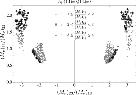
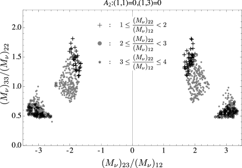
Figure 2: Correlations between $(M_{\nu})_{23}/(M_{\nu})_{13}$ and $(M_{\nu})_{33}/(M_{\nu})_{22}$ (left panel) for the case of A₁, and $(M_{\nu})_{23}/(M_{\nu})_{12}$ and $(M_{\nu})_{33}/(M_{\nu})_{22}$ (right panel) for the case of A₂. The symbols $+$, grey points and $\ast$ represent $1\leq|(M_{\nu})_{22}/(M_{\nu})_{13(12)}|<2$, $2\leq|(M_{\nu})_{22}/(M_{\nu})_{13(12)}|<3$ and $3\leq|(M_{\nu})_{22}/(M_{\nu})_{13(12)}|\leq 4$ for the left (right) panel, respectively.

Next we discuss correlations between non-zero elements of $M_{\nu}$. Figure 2 shows the allowed region in $(M_{\nu})_{23}/(M_{\nu})_{13}-(M_{\nu})_{33}/(M_{\nu})_{22}$ plane (left panel) for the case of A₁, and in $(M_{\nu})_{23}/(M_{\nu})_{12}-(M_{\nu})_{33}/(M_{\nu})_{22}$ plane (right panel) for the case of A₂. In both panels, we have chosen the non-zero elements such that all experimental constraints Eq. (2.9) are satisfied. The symbols $+$, grey points and $\ast$ represent $1\leq|(M_{\nu})_{22}/(M_{\nu})_{13(12)}|<2$, $2\leq|(M_{\nu})_{22}/(M_{\nu})_{13(12)}|<3$ and $3\leq|(M_{\nu})_{22}/(M_{\nu})_{13(12)}|\leq 4$, respectively for the case A₁(A₂). There are no solutions for $|(M_{\nu})_{22}/(M_{\nu})_{13(12)}|<1$ and $4<|(M_{\nu})_{22}/(M_{\nu})_{13(12)}|$. From these figures, one finds solutions at $|(M_{\nu})_{23}/(M_{\nu})_{13(12)}|\sim 2~{}{\rm or}~{}3$, and $0.5\raise 1.29167pt\hbox{$\;<$\kern-7.5pt\raise-4.73611pt\hbox{$\sim\;$}}(M_{\nu})_{33}/(M_{\nu})_{22}\raise 1.29167pt\hbox{$\;<$\kern-7.5pt\raise-4.73611pt\hbox{$\sim\;$}}2$ with $1<|(M_{\nu})_{22}/(M_{\nu})_{13(12)}|<4$.

$M_{\nu}$	$m\left(\begin{array}[]{ccc}0&0&1\\ 0&2&3\\ 1&3&3\\ \end{array}\right)$	$m\left(\begin{array}[]{ccc}0&0&1\\ 0&\sqrt{3}&2\sqrt{2}\\ 1&2\sqrt{2}&2\sqrt{2}\\ \end{array}\right)$	$m\left(\begin{array}[]{ccc}0&0&1\\ 0&\sqrt{3}&2\sqrt{2}\\ 1&2\sqrt{2}&3\\ \end{array}\right)$	$m\left(\begin{array}[]{ccc}0&0&1\\ 0&2&3\\ 1&3&2\sqrt{2}\\ \end{array}\right)$
$U_{PMNS}$	​​$\left(\begin{array}[]{ccc}\!\!\!\!\frac{3+\sqrt{7}}{2\sqrt{7+2\sqrt{7}}}&\!\!\!\!\frac{1}{\sqrt{3}}&\!\!\!\!\frac{3-\sqrt{7}}{2\sqrt{7-2\sqrt{7}}}\\ \!\!\!\!-\frac{1+\sqrt{7}}{2\sqrt{7+2\sqrt{7}}}&\!\!\!\!\frac{1}{\sqrt{3}}&\!\!\!\!-\frac{1-\sqrt{7}}{2\sqrt{7-2\sqrt{7}}}\\ \!\!\!\!\frac{1}{\sqrt{7+2\sqrt{7}}}&\!\!\!\!-\frac{1}{\sqrt{3}}&\!\!\!\!\frac{1}{\sqrt{7-2\sqrt{7}}}\!\!\!\!\\ \end{array}\right)\!\!$	​​$\left(\begin{array}[]{ccc}\!\!\!\!0.815&\!\!\!\!0.560&\!\!\!\!0.147\\ \!\!\!\!-0.518&\!\!\!\!0.592&\!\!\!\!0.617\\ \!\!\!\!0.259&\!\!\!\!-0.579&\!\!\!\!0.773\!\!\!\\ \end{array}\right)$​​	​​$\left(\begin{array}[]{ccc}\!\!\!\!0.803&\!\!\!\!0.578&\!\!\!\!0.145\\ \!\!\!\!-0.534&\!\!\!\!0.589&\!\!\!\!0.606\\ \!\!\!\!0.265&\!\!\!\!-0.565&\!\!\!\!0.782\!\!\!\\ \end{array}\right)$​​	​​$\left(\begin{array}[]{ccc}\!\!\!\!0.819&\!\!\!\!0.559&\!\!\!\!0.136\\ \!\!\!\!-0.504&\!\!\!\!0.581&\!\!\!\!0.640\\ \!\!\!\!0.279&\!\!\!\!0.592&\!\!\!\!0.756\\ \end{array}\right)$​​
$\sin^{2}\theta_{12}$	$\frac{2}{87}(28-5\sqrt{7})=0.3396$	$0.321$	$0.341$	$0.319$
$\sin^{2}\theta_{23}$	$\frac{1}{29}(17-2\sqrt{7})=0.4037$	$0.389$	$0.376$	$0.417$
$\sin^{2}\theta_{13}$	$\frac{1}{3}-\frac{5}{6\sqrt{7}}=0.01836$	$0.0215$	$0.0211$	$0.0186$
$m_{1}$	$(3-\sqrt{7})m$	$0.318m$	$0.330m$	$0.341m$
$m_{2}$	$-m$	$-1.03m$	$-0.977m$	$-1.06m$
$m_{3}$	$(3+\sqrt{7})m$	$5.28m$	$5.38m$	$5.55m$
$\Delta m_{21}^{2}$	$(-15+6\sqrt{7})m^{2}$	$0.966m^{2}$	$0.846m^{2}$	$1.00m^{2}$
$\Delta m_{31}^{2}$	$12\sqrt{7}m^{2}$	$27.7m^{2}$	$28.8m^{2}$	$30.6m^{2}$
​​​​​​$\begin{array}[]{c}|m|\vspace{-2mm}\\ (10^{-3}{\footnotesize\mbox{eV}})\\ \end{array}$​ ​​​​​​​	$[8.95,~{}9.21]$	$[9.06,~{}9.15]$	$[9.10,~{}9.67]$	$[8.62,~{}8.97]$

Table 1: Examples of one-parameter neutrino mass matrix $M_{\nu}$ and related quantities for $|(M_{\nu})_{23}/(M_{\nu})_{13}|\simeq 3$ for the case of A₁.

$M_{\nu}$	$m\left(\begin{array}[]{ccc}0&0&1\\ 0&\sqrt{6}&2\\ 1&2&5/2\\ \end{array}\right)$	$m\left(\begin{array}[]{ccc}0&0&1\\ 0&5/2&2\\ 1&2&5/2\\ \end{array}\right)$	$m\left(\begin{array}[]{ccc}0&0&1\\ 0&2\sqrt{2}&2\\ 1&2&\sqrt{5}\\ \end{array}\right)$	$m\left(\begin{array}[]{ccc}0&0&1\\ 0&2\sqrt{2}&\sqrt{5}\\ 1&\sqrt{5}&2\sqrt{2}\\ \end{array}\right)$
$U_{PMNS}$	​​$\left(\begin{array}[]{ccc}\!\!\!\!0.825&\!\!\!\!0.543&\!\!\!\!0.157\\ \!\!\!\!0.312&\!\!\!\!-0.669&\!\!\!\!0.675\\ \!\!\!\!-0.472&\!\!\!\!0.507&\!\!\!\!0.721\\ \end{array}\right)$​​	​​$\left(\begin{array}[]{ccc}\!\!\!\!0.828&\!\!\!\!0.539&\!\!\!\!0.156\\ \!\!\!\!0.306&\!\!\!\!-0.667&\!\!\!\!0.679\\ \!\!\!\!-0.470&\!\!\!\!0.515&\!\!\!\!0.717\\ \end{array}\right)$​​	​​$\left(\begin{array}[]{ccc}\!\!\!\!0.822&\!\!\!\!0.552&\!\!\!\!0.143\\ \!\!\!\!0.287&\!\!\!\!-0.618&\!\!\!\!0.732\\ \!\!\!\!-0.492&\!\!\!\!0.560&\!\!\!\!0.666\\ \end{array}\right)$ ​​	​​$\left(\begin{array}[]{ccc}\!\!\!\!0.842&\!\!\!\!0.521&\!\!\!\!0.139\\ \!\!\!\!0.299&\!\!\!\!-0.664&\!\!\!\!0.685\\ \!\!\!\!-0.449&\!\!\!\!0.535&\!\!\!\!0.715\\ \end{array}\right)$​​
$\sin^{2}\theta_{12}$	$0.303$	$0.297$	$0.311$	$0.277$
$\sin^{2}\theta_{23}$	$0.467$	$0.473$	$0.547$	$0.478$
$\sin^{2}\theta_{13}$	$0.0247$	$0.0242$	$0.0205$	$0.0192$
$m_{1}$	$-0.572m$	$-0.567m$	$-0.599m$	$-0.533m$
$m_{2}$	$0.933m$	$0.956m$	$1.02m$	$1.03m$
$m_{3}$	$4.59m$	$4.61m$	$4.65m$	$5.16m$
$\Delta m_{21}^{2}$	$0.544m^{2}$	$0.592m^{2}$	$0.671m^{2}$	$0.70m^{2}$
$\Delta m_{31}^{2}$	$20.7m^{2}$	$20.9m^{2}$	$21.3m^{2}$	$26.4m^{2}$
​​​​​​$\begin{array}[]{c}|m|\vspace{-2mm}\\ (10^{-3}{\footnotesize\mbox{eV}})\\ \end{array}$​ ​​​​​​​	$[11.3,~{}11.4]$	$[10.9,~{}11.3]$	$[10.3,~{}11.0]$	$[9.54,~{}10.1]$

Table 2: Examples of one-parameter neutrino mass matrix $M_{\nu}$ and related quantities for $|(M_{\nu})_{23}/(M_{\nu})_{13}|\simeq 2$ for the case of A₁.

From the numerical calculation above, we find some examples of $M_{\nu}$ with one real free parameter $m$ as listed in Table 1 for $|(M_{\nu})_{23}/(M_{\nu})_{13}|\simeq 3$ and in Table 2 for $|(M_{\nu})_{23}/(M_{\nu})_{13}|\simeq 2$ for the case A₁ . The bound of $|m|$ is obtained by the overlap of two constraints of $\Delta m_{21}^{2}$ and $\Delta m_{31}^{2}$ given in Eq.(2.9). One can see that all textures are in agreement with the current experimental bounds at the 3 $\sigma$ level given in Eq.(2.9). In addition to the mass matrices shown in Tables 1 and 2, matrices with different sign are also candidates of one-parameter $M_{\nu}$, such as

$$\left(\begin{array}[]{ccc}0&0&1\\ 0&2&3\\ 1&3&3\\ \end{array}\right)\to\left(\begin{array}[]{ccc}0&0&1\\ 0&2&-3\\ 1&-3&3\\ \end{array}\right),~{}\left(\begin{array}[]{ccc}0&0&1\\ 0&-2&3\\ 1&3&-3\\ \end{array}\right),~{}\left(\begin{array}[]{ccc}0&0&1\\ 0&-2&-3\\ 1&-3&-3\\ \end{array}\right),$$ (2.22)

with the same observables $\sin^{2}\theta_{12,23,13}$, $\Delta m^{2}_{21,31}$ and consequently the same bounds of $|m|$, while the sign of mass eigenvalues $m_{1,2,3}$ and that of the PMNS matrix $U_{PMNS}$ are different. For the case A₂, all mass matrices $M_{\nu}({\rm A}_{2})$ obtained from $M_{\nu}({\rm A}_{1})$ listed in Tables 1, 2 and Eq.(1.2), are also consistent with Eq.(2.9). The PMNS matrix for the case A₂ is given from that for the case A₁ by $U_{PMNS}({\rm A}_{2})=PU_{PMNS}({\rm A}_{1})$, i.e., $\sin^{2}\theta_{23}({\rm A}_{2})=1-\sin^{2}\theta_{23}({\rm A}_{1})$ and the other quantities remain unchanged.

In the next section, we discuss symmetry realization of the mass matrix

$$M_{\nu}=m\left(\begin{array}[]{ccc}0&0&1\\ 0&2&3\\ 1&3&3\\ \end{array}\right),$$ (2.23)

by the binary icosahedral symmetry $A_{5}^{\prime}$, as an example.

3 Symmetry Realization

In this section, we discuss symmetry realization of the one-parameter texture Eq.(2.23) by the binary icosahedral symmetry $A_{5}^{\prime}$ and the Higgs potential of our model.

3.1 Mass Matrices

	$L_{a}$	$e^{c}_{a}$	$\Phi_{0}$	$\Phi_{a}$	$\Phi^{\prime}_{A}$	$\Delta_{A}$
$(SU(2)_{L},U(1)_{Y})$	$({\bf{2}},-1/2)$	$({\bf{1}},1)$	$({\bf{2}},1/2)$	$({\bf{2}},1/2)$	$({\bf{2}},1/2)$	$({\bf{3}},1)$
$A_{5}^{\prime}$	${\bf 3}_{a}$	${\bf 3}_{a}$	${\bf 1}$	${\bf 3}_{a}$	${\bf 5}_{A}$	${\bf 5}_{A}$

Table 3: The particle contents ($a=1-3$ and $A=1-5$).

Now we discuss symmetry realization of the texture given in Eq.(2.23) for neutrino mass matrix. We consider the binary icosahedral symmetry $A_{5}^{\prime}$ [20] as a flavor symmetry. The $A_{5}^{\prime}$ symmetry contains three- and five-dimensional irreducible representations ${\bf 3}$ and ${\bf 5}$, and their tensor product gives $A_{5}^{\prime}$ invariance ${\bf 1}$. Moreover the resultant singlet ${\bf 1}$ from ${\bf 3\cdot 5\cdot 3}$ enters all the elements of $M_{\nu}$ with desired weights if neutrinos and Higgs bosons are embedded into ${\bf 3}$ and ${\bf 5}$, respectively. Therefore the $A_{5}^{\prime}$ symmetry is preferable for the one-parameter texture. For the lepton sector, the particle contents are shown in Table 3, where $L_{a},~{}e^{c}_{a},~{}(\Phi_{0,a},~{}\Phi^{\prime}_{A})$ and $\Delta_{A}$ ($a=1-3,~{}A=1-5$) are the $SU(2)_{L}$ doublet leptons, $SU(2)$ singlet leptons, $SU(2)$ doublet Higgs fields and $SU(2)$ triplet Higgs fields, respectively. Since right-handed neutrinos are absent in our model, the $SU(2)_{L}$ doublet Higgs fields are responsible only for masses of charged leptons, while neutrino masses are generated by the vacuum expectation values (VEVs) of $SU(2)_{L}$ triplet Higgs fields through the type-II seesaw mechanism. If one assigns ${\bf 1}$ for quarks, only $\Phi_{0}$ couples to quarks and gives their masses. Although there are no predictions in the quark sector, it is ensured to be the same as the standard model.

Now we give the multiplication rules of the $A_{5}^{\prime}$ group relevant for the Yukawa interactions in our model. For ${\bf 3}$ and ${\bf 5}$ irreducible representations

$${\bf 3}=\left(\begin{array}[]{c}x_{1}\\ x_{2}\\ x_{3}\\ \end{array}\right),~{}\left(\begin{array}[]{c}y_{1}\\ y_{2}\\ y_{3}\\ \end{array}\right),~{}{\bf 5}=\left(\begin{array}[]{c}X_{1}\\ X_{2}\\ X_{3}\\ X_{4}\\ X_{5}\\ \end{array}\right),~{}\left(\begin{array}[]{c}Y_{1}\\ Y_{2}\\ Y_{3}\\ Y_{4}\\ Y_{5}\\ \end{array}\right),$$ (3.17)

their tensor products are given by

$${\bf 3}\otimes{\bf 3}=\left(x_{1}y_{3}-x_{2}y_{2}+x_{3}y_{1}\right)_{{\bf 1}}+\frac{1}{\sqrt{2}}\left(\begin{array}[]{c}x_{1}y_{2}-x_{2}y_{1}\\ x_{1}y_{3}-x_{3}y_{1}\\ x_{2}y_{3}-x_{3}y_{2}\end{array}\right)_{{\bf 3}}+\left(\begin{array}[]{c}x_{1}y_{1}\\ \frac{1}{\sqrt{2}}\left(x_{1}y_{2}+x_{2}y_{1}\right)\\ \frac{1}{\sqrt{6}}\left(x_{1}y_{3}+2x_{2}y_{2}+x_{3}y_{1}\right)\\ \frac{1}{\sqrt{2}}\left(x_{2}y_{3}+x_{3}y_{2}\right)\\ x_{3}y_{3}\\ \end{array}\right)_{{\bf 5}},$$ (3.26)

$${\bf 5}\otimes{\bf 5}=\left(X_{1}Y_{5}-X_{2}Y_{4}+X_{3}Y_{3}-X_{4}Y_{2}+X_{5}Y_{1}\right)_{\bf 1}+\cdots.$$ (3.27)

From the particle contents shown in Table 3 and the multiplication rules Eq. (3.27), the $A_{5}^{\prime}$ invariant Yukawa interactions are given by

$${\cal L}_{Y} = y_{\Delta}L_{a}^{T}i\sigma_{2}\Delta_{A}L_{b}+y_{1}\Phi_{0}^{{\dagger}}L_{a}e_{b}^{c}+y_{2}\Phi_{a}^{{\dagger}}L_{b}e_{c}^{c}+y_{3}{\Phi^{\prime}}_{A}^{{\dagger}}L_{a}e_{b}^{c}+c.c.,$$ (3.28)

where all indices are summed up in $A_{5}^{\prime}$ invariant way in accordance with Eq(3.27). After the electroweak symmetry breaking by the VEVs of the Higgs fields defined by

$$\langle\Delta_{A}\rangle=\frac{1}{\sqrt{2}}v_{\Delta A},~{}~{}\langle\Phi_{0,a}\rangle=\frac{1}{\sqrt{2}}v_{0,a},~{}~{}\langle\Phi^{\prime}_{A}\rangle=\frac{1}{\sqrt{2}}V_{A},$$ (3.29)

with $v_{0}^{2}+\sum_{a}v_{a}^{2}+\sum_{A}(V_{A}^{2}+2v_{\Delta A}^{2})=(246\mbox{GeV})^{2}$ , we obtain the following mass matrix

$$M_{\nu}=\frac{y_{\Delta}}{\sqrt{2}}\left(\begin{array}[]{ccc}v_{\Delta 5}&-\frac{1}{\sqrt{2}}v_{\Delta 4}&\frac{1}{\sqrt{6}}v_{\Delta 3}\\ -\frac{1}{\sqrt{2}}v_{\Delta 4}&\frac{2}{\sqrt{6}}v_{\Delta 3}&-\frac{1}{\sqrt{2}}v_{\Delta 2}\\ \frac{1}{\sqrt{6}}v_{\Delta 3}&-\frac{1}{\sqrt{2}}v_{\Delta 2}&v_{\Delta 1}\\ \end{array}\right),$$ (3.30)

for neutrino sector, and

$$M_{e}=\frac{1}{\sqrt{2}}\left(\begin{array}[]{ccc}y_{3}V_{5}&\frac{1}{\sqrt{2}}y_{2}v_{3}-\frac{1}{\sqrt{2}}y_{3}V_{4}&y_{1}v_{0}-\frac{1}{\sqrt{2}}y_{2}v_{2}+\frac{1}{\sqrt{6}}y_{3}V_{3}\\ -\frac{1}{\sqrt{2}}y_{2}v_{3}-\frac{1}{\sqrt{2}}y_{3}V_{4}&-y_{1}v_{0}+\frac{2}{{\sqrt{6}}}y_{3}V_{3}&\frac{1}{\sqrt{2}}y_{2}v_{1}-\frac{1}{\sqrt{2}}y_{3}V_{2}\\ y_{1}v_{0}+\frac{1}{\sqrt{2}}y_{2}v_{2}+\frac{1}{\sqrt{6}}y_{3}V_{3}&-\frac{1}{\sqrt{2}}y_{2}v_{1}-\frac{1}{\sqrt{2}}y_{3}V_{2}&y_{3}V_{1}\\ \end{array}\right),$$ (3.31)

for charged lepton sector. If the Higgs fields obtain the following VEVs,

$$v_{\Delta 1}=3v_{\Delta},~{}v_{\Delta 2}=-3\sqrt{2}v_{\Delta},~{}v_{\Delta 3}=\sqrt{6}v_{\Delta},~{}v_{\Delta 4}=v_{\Delta 5}=0,$$

$$v_{0}\neq 0,~{}v_{2}\neq 0,~{}V_{3}\neq 0,~{}v_{1}=v_{3}=V_{1}=V_{2}=V_{4}=V_{5}=0,~{}$$ (3.32)

one finds that the mass matrices $M_{\nu}$ and $M_{e}$ have the desired form

$$M_{\nu}=\frac{y_{\Delta}v_{\Delta}}{\sqrt{2}}\left(\begin{array}[]{ccc}0&0&1\\ 0&2&3\\ 1&3&3\\ \end{array}\right),~{}~{}~{}M_{e}=\left(\begin{array}[]{ccc}0&0&m_{e}\\ 0&-m_{\mu}&0\\ m_{\tau}&0&0\\ \end{array}\right),$$ (3.33)

where

$$m_{e}=\frac{1}{\sqrt{2}}\left(y_{1}v_{0}-\frac{1}{\sqrt{2}}y_{2}v_{2}+\frac{1}{\sqrt{6}}y_{3}V_{3}\right),$$ (3.34)

$$m_{\mu}=\frac{1}{\sqrt{2}}\left(y_{1}v_{0}-\frac{2}{\sqrt{6}}y_{3}V_{3}\right),$$ (3.35)

$$m_{\tau}=\frac{1}{\sqrt{2}}\left(y_{1}v_{0}+\frac{1}{\sqrt{2}}y_{2}v_{2}+\frac{1}{\sqrt{6}}y_{3}V_{3}\right),$$ (3.36)

and $M_{e}M_{e}^{{\dagger}}={\rm diag}(m_{e}^{2},~{}m_{\mu}^{2},~{}m_{\tau}^{2})$. The VEVs of the triplet Higgs $\Delta_{A}$ gives additional contributions to the $\rho$ parameter

$$\rho=\frac{v^{2}}{v^{2}+2\sum_{A}v_{\Delta A}^{2}}=\frac{v^{2}}{v^{2}+66v_{\Delta}^{2}},$$ (3.37)

where $v^{2}=v_{0}^{2}+\sum_{a}v_{a}^{2}+\sum_{A}V_{A}^{2}=v_{0}^{2}+v_{2}^{2}+V_{3}^{2}$ because of Eq. (3.32). The experimental value $\rho_{\rm exp}=1.0004^{+0.0003}_{-0.0004}$ constrains $v_{\Delta}$ to be smaller than about $0.61\mbox{GeV}$ at the 95$\%$ confidence level. Therefore we assume $v_{\Delta}\ll v_{0},v_{2},V_{3}$. As already discussed in the last section, the mass matrices Eq.(3.33) with $m=y_{\Delta}v_{\Delta}/\sqrt{2}$ corresponding to Eq.(2.23) are compatible with the current experimental bounds.

3.2 Higgs Sector

As for the Higgs sector, the total Higgs potential is given in Appendix in symbolic form. Here we mention the tadpole conditions. The $A^{\prime}_{5}$ invariant scalar mass terms are given by

$$V_{\rm mass}=m_{0}^{2}\Phi_{0}^{{\dagger}}\Phi_{0}+m_{3}^{2}\left(\Phi_{1}^{{\dagger}}\Phi_{3}-\Phi_{2}^{{\dagger}}\Phi_{2}+\Phi_{3}^{{\dagger}}\Phi_{1}\right)$$

$$+m_{5}^{2}\left({\Phi^{\prime}}_{1}^{{\dagger}}\Phi^{\prime}_{5}-{\Phi^{\prime}}_{2}^{{\dagger}}\Phi^{\prime}_{4}+{\Phi^{\prime}}_{3}^{{\dagger}}\Phi^{\prime}_{3}-{\Phi^{\prime}}_{4}^{{\dagger}}\Phi^{\prime}_{2}+{\Phi^{\prime}}_{5}^{{\dagger}}\Phi^{\prime}_{1}\right)$$

$$+m_{\Delta}^{2}{\rm Tr}\left[\Delta_{1}^{{\dagger}}\Delta_{5}-\Delta_{2}^{{\dagger}}\Delta_{4}+\Delta_{3}^{{\dagger}}\Delta_{3}-\Delta_{4}^{{\dagger}}\Delta_{2}+\Delta_{5}^{{\dagger}}\Delta_{1}\right].$$ (3.38)

Since the total $A^{\prime}_{5}$ invariant potential does not have any accidental symmetry, our model does not suffer from the problem of massless Goldstone bosons.

By imposing the conditions for the VEVs Eq.(3.32), the tadpole conditions give the scalar masses

$$m_{0}^{2} \simeq -\lambda_{1}v_{0}^{2}+\left(\frac{1}{2}\tilde{\epsilon}_{1}-\frac{V_{3}}{\sqrt{6}v_{0}}\tilde{\kappa}_{8}\right)v_{2}^{2}-\frac{1}{2}\left(\tilde{\epsilon}_{2}-\frac{V_{3}}{v_{0}}\kappa_{2}^{(1)}\right)V_{3}^{2},$$ (3.39)

$$m_{3}^{2} \simeq -\frac{1}{2}\tilde{\epsilon}_{1}v_{0}^{2}+\left(\lambda_{2}^{(1)}+\frac{2}{3}\lambda_{2}^{(3)}\right)v_{2}^{2}-\left(\tilde{\epsilon}_{4}+2\tilde{\epsilon}_{5}+\tilde{\epsilon}_{6}\right)V_{3}^{2}+\frac{\sqrt{6}}{3}\tilde{\kappa}_{8}v_{0}V_{3}-2\sqrt{2}v_{\Delta}\mu_{1},$$ (3.40)

$$m_{5}^{2} \simeq -\frac{1}{2}\tilde{\epsilon}_{2}v_{0}^{2}+\left(\tilde{\epsilon}_{4}+2\tilde{\epsilon}_{5}+\tilde{\epsilon}_{6}-\frac{v_{0}}{\sqrt{6}V_{3}}\tilde{\kappa}_{8}\right)v_{2}^{2}-\tilde{\lambda}_{3}V_{3}^{2}+\frac{3}{2}\kappa_{2}^{(1)}v_{0}V_{3}-2\sqrt{3}v_{\Delta}\left(\mu_{2}-6\mu_{3}\right),$$ (3.41)

$$m_{\Delta}^{2} \simeq -\frac{1}{2}\tilde{\epsilon}_{3}v_{0}^{2}+\left(\tilde{\epsilon}_{7}+\tilde{\epsilon}_{8}+\frac{\mu_{1}}{3\sqrt{2}v_{\Delta}}\right)v_{2}^{2}-\frac{1}{2}\left(\tilde{\lambda}_{4}+\tilde{\lambda}_{5}+\frac{\mu_{2}-6\mu_{3}}{\sqrt{3}v_{\Delta}}\right)V_{3}^{2}+\tilde{\kappa}_{2}v_{0}V_{3},$$ (3.42)

where

$$\tilde{\lambda}_{i} = \lambda_{i}^{(1)}-\lambda_{i}^{(7)}-6\lambda_{i}^{(8)}+36\lambda_{i}^{(9)}~{}(i=3,4,5),$$

$$\tilde{\epsilon}_{i} = \epsilon_{i}^{(1)}+\epsilon_{i}^{(2)}+2\epsilon_{i}^{(3)}~{}(i=1,2),~{}\tilde{\epsilon}_{3}=\epsilon_{3}^{(1)}+\epsilon_{3}^{(2)},~{}\tilde{\epsilon}_{i}=\frac{1}{2}\epsilon_{i}^{(1)}+\frac{1}{\sqrt{6}}\epsilon_{i}^{(3)}+\frac{3}{10}\epsilon_{i}^{(4)}~{}(i=4,5,6,7,8),$$

$$\tilde{\kappa}_{2} = \kappa_{2}^{(2)}+\kappa_{2}^{(3)},~{}\tilde{\kappa}_{8}=\kappa_{8}^{(1)}+\kappa_{8}^{(2)}+\kappa_{8}^{(3)}.$$ (3.43)

The coupling constants $\lambda$s, $\epsilon$s and $\kappa$s are given in Appendix. In Eqs. (3.39)-(3.42), the terms proportional to $v_{\Delta}^{2}$ have been neglected. The pattern

$$M_{\nu}=\left(\begin{array}[]{ccc}0&0&1\\ 0&2&3\\ 1&3&2\sqrt{2}\\ \end{array}\right),$$ (3.44)

listed in Table 1 can be realized by the $A_{5}^{\prime}$ symmetry in similar fashion, with corresponding tadpole conditions.

4 Conclusions

We have studied neutrino mass matrix $M_{\nu}$ with two texture zeros and its symmetry realization. After confirming that the cases A₁ and A₂ satisfy the current experimental constraints by numerical calculation, we have found some examples of $M_{\nu}$ with one real parameter. Since the magnitude of non-zero elements of $M_{\nu}$ is restricted in small region, one can extract examples of $M_{\nu}$ with simple forms. While there exist infinite number of candidates of one-parameter $M_{\nu}$, such simple forms are preferable in the standpoint of flavor symmetry.

Next we have discussed symmetry realization of one-parameter $M_{\nu}$ and the Higgs potential based on the binary icosahedral symmetry $A_{5}^{\prime}$. The $A_{5}^{\prime}$ symmetry contains three- and five-dimensional irreducible representations, and their tensor product ${\bf 3\cdot 5\cdot 3}$ enters all the elements of $M_{\nu}$ with definite weights. If one assigns ${\bf 5}$ to $SU(2)_{L}$ triplet Higgs $\Delta$, desired neutrino mass matrix is obtained by the type-II seesaw mechanism and by choosing the vacua of the Higgs potential. While we have shown one example of symmetry realization in this paper, the $A_{5}^{\prime}$ symmetry can work for the other one-parameter $M_{\nu}$ because of its multiplication rules.

Appendix A Higgs Potential

Here we show the Higgs potential of our model with the A${}_{5}^{\prime}$ symmetry. In order to avoid redundancy, we give a symbolic form of the potential. The Higgs fields are denoted by

$$\Phi_{0}\equiv{\bf 1},~{}\Phi_{a}\equiv{\bf 3},~{}\Phi^{\prime}_{A}\equiv{\bf 5},~{}\Delta_{A}\equiv\Delta$$ (A.1)

where $a=1-3$ and $A=1-5$ for three- and five- dimensional representation, respectively. Their Hermitian conjugate fields are denoted by $\Phi_{a}^{{\dagger}}\equiv{\bf 3}^{{\dagger}}$ etc., while ${\bf 3}^{{\dagger}}$ and ${\bf 3}$ obey the same multiplication rules. We represent a product

$${\bf 3}\otimes{\bf 3}={\bf 1}\oplus{\bf 3}\oplus{\bf 5}~{} \rightarrow ~{}{\bf 33}=({\bf 33})_{\bf 1}+({\bf 33})_{\bf 3}+({\bf 33})_{\bf 5}=({\bf 33})_{\alpha},$$ (A.2)

$${\rm or} ~{}{\bf 3^{{\dagger}}3}=({\bf 3^{{\dagger}}3})_{\bf 1}+({\bf 3^{{\dagger}}3})_{\bf 3}+({\bf 3^{{\dagger}}3})_{\bf 5}=({\bf 3^{{\dagger}}3})_{\alpha},$$

depending on the gauge quantum number of the Higgs fields. The index $\alpha$ must be summed up for all possible combinations of the tensor product. For example in the case of $({\bf 3^{{\dagger}}3})^{2}$, since only the products ${\bf 11},~{}{\bf 33}$ and ${\bf 55}$ can be invariant under A${}_{5}^{\prime}$, we denote $\lambda_{2}^{(\alpha)}({\bf 3}^{{\dagger}}{\bf 3})_{\alpha}({\bf 3}^{{\dagger}}{\bf 3})_{\alpha}$ as

$$({\bf 3^{{\dagger}}3})^{2}~{}:~{}\lambda_{2}^{(\alpha)}({\bf 3}^{{\dagger}}{\bf 3})_{\alpha}({\bf 3}^{{\dagger}}{\bf 3})_{\alpha}=\lambda_{2}^{(1)}({\bf 3}^{{\dagger}}{\bf 3})_{\bf 1}({\bf 3}^{{\dagger}}{\bf 3})_{\bf 1}+\lambda_{2}^{(2)}({\bf 3}^{{\dagger}}{\bf 3})_{\bf 3}({\bf 3}^{{\dagger}}{\bf 3})_{\bf 3}+\lambda_{2}^{(3)}({\bf 3}^{{\dagger}}{\bf 3})_{\bf 5}({\bf 3}^{{\dagger}}{\bf 3})_{\bf 5}$$

$$=\lambda_{2}^{(1)}\left(\Phi_{1}^{{\dagger}}\Phi_{3}-\Phi_{2}^{{\dagger}}\Phi_{2}+\Phi_{3}^{{\dagger}}\Phi_{1}\right)^{2}$$

$$+\lambda_{2}^{(2)}\left[2\left(\Phi_{1}^{{\dagger}}\Phi_{2}-\Phi_{2}^{{\dagger}}\Phi_{1}\right)\left(\Phi_{2}^{{\dagger}}\Phi_{3}-\Phi_{3}^{{\dagger}}\Phi_{2}\right)-\left(\Phi_{1}^{{\dagger}}\Phi_{3}-\Phi_{3}^{{\dagger}}\Phi_{1}\right)^{2}\right]$$

$$+\lambda_{2}^{(3)}\left[2\left(\Phi_{1}^{{\dagger}}\Phi_{1}\right)\left(\Phi_{3}^{{\dagger}}\Phi_{3}\right)-\left(\Phi_{1}^{{\dagger}}\Phi_{2}+\Phi_{2}^{{\dagger}}\Phi_{1}\right)\left(\Phi_{2}^{{\dagger}}\Phi_{3}+\Phi_{3}^{{\dagger}}\Phi_{2}\right)+\frac{1}{6}\left(\Phi_{1}^{{\dagger}}\Phi_{3}+\Phi_{2}^{{\dagger}}\Phi_{2}+\Phi_{3}^{{\dagger}}\Phi_{1}\right)^{2}\right].$$

Moreover in what follows, trace for $\Delta$ is omitted, and “ $\cdot$ ” denotes the Pauli matrices $\sigma^{1,2,3}$.

In the notation described above, the Higgs potential except the bilinear terms given in the main text can be written down as

$${\bf 3}^{2}{\bf 5},{\bf 5}^{3},{\bf 3}{\bf 5}^{2} : \mu_{1}{\bf 3}\Delta^{{\dagger}}{\bf 3}+\mu_{2}({\bf 5}\Delta^{{\dagger}})_{\bf 5_{1}}{\bf 5}+\mu_{3}({\bf 5}\Delta^{{\dagger}})_{\bf 5_{2}}{\bf 5}+\mu_{4}{\bf 3}\Delta^{{\dagger}}{\bf 5}+h.c.,$$ (A.4)

for the trilinear terms, and

$${\bf 1}^{4} : \lambda_{1}({\bf 1}^{{\dagger}}{\bf 1})^{2},$$

$${\bf 3}^{4} : \lambda_{2}^{(\alpha)}({\bf 3}^{{\dagger}}{\bf 3})_{\alpha}({\bf 3}^{{\dagger}}{\bf 3})_{\alpha},$$

$${\bf 5}^{4} : \lambda_{3}^{(\alpha)}({\bf 5}^{{\dagger}}{\bf 5})_{\alpha}({\bf 5}^{{\dagger}}{\bf 5})_{\alpha}+\lambda_{4}^{(\alpha)}({\bf 5}^{{\dagger}}{\bf 5})_{\alpha}({\Delta}^{{\dagger}}{\Delta})_{\alpha}+\lambda_{5}^{(\alpha)}({\bf 5}^{{\dagger}}\cdot{\bf 5})_{\alpha}({\Delta}^{{\dagger}}\cdot{\Delta})_{\alpha}$$

$$+\lambda_{6}^{(\alpha)}((\Delta^{{\dagger}}\Delta)_{\alpha})^{2}+\lambda_{7}\det\left[\Delta^{{\dagger}}\Delta\right],$$

$${\bf 1}^{2}{\bf 3}^{2} : \epsilon_{1}^{(1)}({\bf 1}^{{\dagger}}{\bf 1})_{{\bf 1}}({\bf 3}^{{\dagger}}{\bf 3})_{{\bf 1}}+\epsilon_{1}^{(2)}({\bf 1}^{{\dagger}}{\bf 3})_{{\bf 3}}({\bf 3}^{{\dagger}}{\bf 1})_{{\bf 3}}+\epsilon_{1}^{(3)}\left[(({\bf 1}^{{\dagger}}{\bf 3})_{{\bf 3}})^{2}+h.c.\right],$$

$${\bf 1}^{2}{\bf 5}^{2} : \epsilon_{2}^{(1)}({\bf 1}^{{\dagger}}{\bf 1})_{{\bf 1}}({\bf 5}^{{\dagger}}{\bf 5})_{{\bf 1}}+\epsilon_{2}^{(2)}({\bf 1}^{{\dagger}}{\bf 5})_{{\bf 5}}({\bf 5}^{{\dagger}}{\bf 1})_{{\bf 5}}+\epsilon_{2}^{(3)}\left[(({\bf 1}^{{\dagger}}{\bf 5})_{{\bf 5}})^{2}+h.c.\right]$$

$$+\epsilon_{3}^{(1)}({\bf 1}^{{\dagger}}{\bf 1})_{{\bf 1}}(\Delta^{{\dagger}}\Delta)_{\bf 1}+\epsilon_{3}^{(2)}({\bf 1}^{{\dagger}}\cdot{\bf 1})_{{\bf 1}}(\Delta^{{\dagger}}\cdot\Delta)_{\bf 1},$$

$${\bf 3}^{2}{\bf 5}^{2} : \epsilon_{4}^{(\alpha)}({\bf 3}^{{\dagger}}{\bf 3})_{\alpha}({\bf 5}^{{\dagger}}{\bf 5})_{\alpha}+\epsilon_{5}^{(\alpha)}\left[(({\bf 3}^{{\dagger}}{\bf 5})_{\alpha})^{2}+h.c.\right]+\epsilon_{6}^{(\alpha)}({\bf 3}^{{\dagger}}{\bf 5})_{\alpha}({\bf 5}^{{\dagger}}{\bf 3})_{\alpha}$$

$$+\epsilon_{7}^{(\alpha)}({\bf 3}^{{\dagger}}{\bf 3})_{\alpha}(\Delta^{{\dagger}}\Delta)_{\alpha}+\epsilon_{8}^{(\alpha)}({\bf 3}^{{\dagger}}\cdot{\bf 3})_{\alpha}(\Delta^{{\dagger}}\cdot\Delta)_{\alpha}$$

$${\bf 1}{\bf 3}^{3} : \kappa_{1}({\bf 1}^{{\dagger}}{\bf 3})_{\bf 3}({\bf 3}^{{\dagger}}{\bf 3})_{\bf 3}+h.c.,$$

$${\bf 1}{\bf 5}^{3} : \kappa_{2}^{(1)}({\bf 1}^{{\dagger}}{\bf 5})_{\bf 5}({\bf 5}^{{\dagger}}{\bf 5})_{\bf 5}+\kappa_{2}^{(2)}({\bf 1}^{{\dagger}}{\bf 5})_{\bf 5}(\Delta^{{\dagger}}\Delta)_{\bf 5}+\kappa_{2}^{(3)}({\bf 1}^{{\dagger}}\cdot{\bf 5})_{\bf 5}(\Delta^{{\dagger}}\cdot\Delta)_{\bf 5}+h.c.,$$

$${\bf 3}^{3}{\bf 5} : \kappa_{3}^{(1)}({\bf 3}^{{\dagger}}{\bf 3})_{\bf 3}({\bf 3}^{{\dagger}}{\bf 5})_{\bf 3}+\kappa_{3}^{(2)}({\bf 3}^{{\dagger}}{\bf 3})_{\bf 5}({\bf 3}^{{\dagger}}{\bf 5})_{\bf 5}+h.c.,$$

$${\bf 3}{\bf 5}^{3} : \kappa_{4}^{(\alpha)}({\bf 3}^{{\dagger}}{\bf 5})_{\alpha}({\bf 5}^{{\dagger}}{\bf 5})_{\alpha}+\kappa_{5}^{(\alpha)}({\bf 3}^{{\dagger}}{\bf 5})_{\alpha}(\Delta^{{\dagger}}\Delta)_{\alpha}+\kappa_{6}^{(\alpha)}({\bf 3}^{{\dagger}}\cdot{\bf 5})_{\alpha}(\Delta^{{\dagger}}\cdot\Delta)_{\alpha}+h.c.,$$

$${\bf 1}{\bf 3}{\bf 5}^{2} : \kappa_{7}^{(1)}({\bf 1}^{{\dagger}}{\bf 3})_{\bf 3}({\bf 5}^{{\dagger}}{\bf 5})_{\bf 3}+\kappa_{7}^{(2)}({\bf 1}^{{\dagger}}{\bf 5})_{\bf 5}({\bf 3}^{{\dagger}}{\bf 5})_{\bf 5}+\kappa_{7}^{(3)}({\bf 1}^{{\dagger}}{\bf 5})_{\bf 5}({\bf 5}^{{\dagger}}{\bf 3})_{\bf 5}$$

$$+\kappa_{7}^{(4)}({\bf 1}^{{\dagger}}{\bf 3})_{\bf 3}(\Delta^{{\dagger}}\Delta)_{\bf 3}+\kappa_{7}^{(5)}({\bf 1}^{{\dagger}}\cdot{\bf 3})_{\bf 3}(\Delta^{{\dagger}}\cdot\Delta)_{\bf 3}+h.c.,$$

$${\bf 1}{\bf 3}^{2}{\bf 5} : \kappa_{8}^{(1)}({\bf 1}^{{\dagger}}{\bf 3})_{\bf 3}({\bf 3}^{{\dagger}}{\bf 5})_{\bf 3}+\kappa_{8}^{(2)}({\bf 1}^{{\dagger}}{\bf 3})_{\bf 3}({\bf 5}^{{\dagger}}{\bf 3})_{\bf 3}+\kappa_{8}^{(3)}({\bf 1}^{{\dagger}}{\bf 5})_{\bf 5}({\bf 3}^{{\dagger}}{\bf 3})_{\bf 5}+h.c.,$$ (A.5)

for the quartic terms. In the above expressions, the sums of index $\alpha$ are defined as

$${\bf 3}^{4}~{}:~{}\lambda_{2}^{(\alpha)}({\bf 3}^{{\dagger}}{\bf 3})_{\alpha}({\bf 3}^{{\dagger}}{\bf 3})_{\alpha}=\lambda_{2}^{(1)}({\bf 3}^{{\dagger}}{\bf 3})_{\bf 1}({\bf 3}^{{\dagger}}{\bf 3})_{\bf 1}+\lambda_{2}^{(2)}({\bf 3}^{{\dagger}}{\bf 3})_{\bf 3}({\bf 3}^{{\dagger}}{\bf 3})_{\bf 3}+\lambda_{2}^{(3)}({\bf 3}^{{\dagger}}{\bf 3})_{\bf 5}({\bf 3}^{{\dagger}}{\bf 3})_{\bf 5}$$

$${\bf 5}^{4}~{}:~{}\lambda^{(\alpha)}({\bf 5}^{{\dagger}}{\bf 5})_{\alpha}({\bf 5}^{{\dagger}}{\bf 5})_{\alpha}=\lambda^{(1)}({\bf 5}^{{\dagger}}{\bf 5})_{\bf 1}({\bf 5}^{{\dagger}}{\bf 5})_{\bf 1}+\lambda^{(2)}({\bf 5}^{{\dagger}}{\bf 5})_{\bf 3}({\bf 5}^{{\dagger}}{\bf 5})_{\bf 3}+\lambda^{(3)}({\bf 5}^{{\dagger}}{\bf 5})_{\bf 3^{\prime}}({\bf 5}^{{\dagger}}{\bf 5})_{\bf 3^{\prime}}$$

$$\hskip 122.34692pt+\lambda^{(4)}({\bf 5}^{{\dagger}}{\bf 5})_{\bf 4_{1}}({\bf 5}^{{\dagger}}{\bf 5})_{\bf 4_{1}}+\lambda^{(5)}({\bf 5}^{{\dagger}}{\bf 5})_{\bf 4_{1}}({\bf 5}^{{\dagger}}{\bf 5})_{\bf 4_{2}}+\lambda^{(6)}({\bf 5}^{{\dagger}}{\bf 5})_{\bf 4_{2}}({\bf 5}^{{\dagger}}{\bf 5})_{\bf 4_{2}}$$

$$\hskip 122.34692pt+\lambda^{(7)}({\bf 5}^{{\dagger}}{\bf 5})_{\bf 5_{1}}({\bf 5}^{{\dagger}}{\bf 5})_{\bf 5_{1}}+\lambda^{(8)}({\bf 5}^{{\dagger}}{\bf 5})_{\bf 5_{1}}({\bf 5}^{{\dagger}}{\bf 5})_{\bf 5_{2}}+\lambda^{(9)}({\bf 5}^{{\dagger}}{\bf 5})_{\bf 5_{2}}({\bf 5}^{{\dagger}}{\bf 5})_{\bf 5_{2}}$$

$${\bf 3}^{2}{\bf 5}^{2}~{}:~{}\epsilon^{(\alpha)}({\bf 3^{{\dagger}}3})_{\alpha}({\bf 5^{{\dagger}}5})_{\alpha}=\epsilon^{(1)}({\bf 3^{{\dagger}}3})_{\bf 1}({\bf 5^{{\dagger}}5})_{\bf 1}+\epsilon^{(2)}({\bf 3^{{\dagger}}3})_{\bf 3}({\bf 5^{{\dagger}}5})_{\bf 3}+\epsilon^{(3)}({\bf 3^{{\dagger}}3})_{\bf 5}({\bf 5^{{\dagger}}5})_{\bf 5}$$

$$\hskip 130.88284pt+\epsilon^{(4)}({\bf 3^{{\dagger}}3})_{\bf 3^{\prime}}({\bf 5^{{\dagger}}5})_{\bf 3^{\prime}}+\epsilon^{(5)}({\bf 3^{{\dagger}}3})_{\bf 4}({\bf 5^{{\dagger}}5})_{\bf 4}$$

$${\bf 3}{\bf 5}^{3}~{}:~{}\kappa^{(\alpha)}({\bf 3}^{{\dagger}}{\bf 5})_{\alpha}({\bf 5}^{{\dagger}}{\bf 5})_{\alpha}=\kappa^{(1)}({\bf 3}^{{\dagger}}{\bf 5})_{\bf 3}({\bf 5}^{{\dagger}}{\bf 5})_{\bf 3}+\kappa^{(2)}({\bf 3}^{{\dagger}}{\bf 5})_{\bf 3^{\prime}}({\bf 5}^{{\dagger}}{\bf 5})_{\bf 3^{\prime}}+\kappa^{(3)}({\bf 3}^{{\dagger}}{\bf 5})_{\bf 4}({\bf 5}^{{\dagger}}{\bf 5})_{\bf 4_{1}}$$

$$\hskip 130.88284pt+\kappa^{(4)}({\bf 3}^{{\dagger}}{\bf 5})_{\bf 4}({\bf 5}^{{\dagger}}{\bf 5})_{\bf 4_{2}}+\kappa^{(5)}({\bf 3}^{{\dagger}}{\bf 5})_{\bf 5}({\bf 5}^{{\dagger}}{\bf 5})_{\bf 5_{1}}+\kappa^{(6)}({\bf 3}^{{\dagger}}{\bf 5})_{\bf 5}({\bf 5}^{{\dagger}}{\bf 5})_{\bf 5_{2}}.$$ (A.6)

Here notice that the product ${\bf 55}$ contains two ${\bf 4}(={\bf 4_{1},4_{2}})$ and ${\bf 5}(={\bf 5_{1},5_{2}})$. See Ref.[20] for details.

References

- [1] K. Abe et al. [T2K Collaboration], Phys. Rev. Lett. 107, 041801 (2011) [arXiv:1106.2822 [hep-ex]].
- [2] P. Adamson et al. [MINOS Collaboration], Phys. Rev. Lett. 107, 181802 (2011) [arXiv:1108.0015 [hep-ex]].
- [3] Y. Abe et al. [DOUBLE-CHOOZ Collaboration], Phys. Rev. Lett. 108, 131801 (2012) [arXiv:1112.6353 [hep-ex]].
- [4] F. P. An et al. [DAYA-BAY Collaboration], Phys. Rev. Lett. 108, 171803 (2012) [arXiv:1203.1669 [hep-ex]].
- [5] J. K. Ahn et al. [RENO Collaboration], Phys. Rev. Lett. 108, 191802 (2012) [arXiv:1204.0626 [hep-ex]].
- [6] P. F. Harrison, D. H. Perkins and W. G. Scott, Phys. Lett. B 530, 167 (2002) [hep-ph/0202074]; P. F. Harrison and W. G. Scott, Phys. Lett. B 535, 163 (2002) [hep-ph/0203209]; P. F. Harrison and W. G. Scott, Phys. Lett. B 557, 76 (2003) [hep-ph/0302025]; P. F. Harrison and W. G. Scott, hep-ph/0402006.
- [7] G. Altarelli and F. Feruglio, Rev. Mod. Phys. 82, 2701 (2010) [arXiv:1002.0211 [hep-ph]].
- [8] H. Ishimori, T. Kobayashi, H. Ohki, Y. Shimizu, H. Okada and M. Tanimoto, Prog. Theor. Phys. Suppl. 183, 1 (2010) [arXiv:1003.3552 [hep-th]]; H. Ishimori, T. Kobayashi, H. Ohki, H. Okada, Y. Shimizu and M. Tanimoto, Lect. Notes Phys. 858, 1 (2012); H. Ishimori, T. Kobayashi, Y. Shimizu, H. Ohki, H. Okada and M. Tanimoto, Fortsch. Phys. 61, 441 (2013).
- [9] L. L. Everett and A. J. Stuart, Phys. Rev. D 79, 085005 (2009) [arXiv:0812.1057 [hep-ph]].
- [10] B. Wang, J. Tang and X. -Q. Li, arXiv:1303.1592 [hep-ph].
- [11] E. I. Lashin and N. Chamoun, Phys. Rev. D 85, 113011 (2012) [arXiv:1108.4010 [hep-ph]].
- [12] P. H. Frampton, S. L. Glashow and D. Marfatia, Phys. Lett. B 536, 79 (2002) [hep-ph/0201008].
- [13] D. Meloni and G. Blankenburg, Nucl. Phys. B 867, 749 (2013) [arXiv:1204.2706 [hep-ph]].
- [14] W. Grimus and P. O. Ludl, J. Phys. G 40, 055003 (2013) [arXiv:1208.4515 [hep-ph]]; W. Grimus and P. O. Ludl, arXiv:1309.7883 [hep-ph].
- [15] H. Fritzsch, Z. -z. Xing and S. Zhou, JHEP 1109, 083 (2011) [arXiv:1108.4534 [hep-ph]]; H. Fritzsch and S. Zhou, Phys. Lett. B 718, 1457 (2013) [arXiv:1212.0411 [hep-ph]].
- [16] L. J. Hall, H. Murayama and N. Weiner, Phys. Rev. Lett. 84, 2572 (2000) [hep-ph/9911341]; N. Haba and H. Murayama, Phys. Rev. D 63, 053010 (2001) [hep-ph/0009174].
- [17] J. Gluza and R. Szafron, Phys. Rev. D 85, 047701 (2012) [arXiv:1111.7278 [hep-ph]]; G. Altarelli, F. Feruglio, I. Masina and L. Merlo, JHEP 1211, 139 (2012) [arXiv:1207.0587 [hep-ph]]; A. de Gouvea and H. Murayama, arXiv:1204.1249 [hep-ph].
- [18] L. Lavoura, Phys. Lett. B 609, 317 (2005) [hep-ph/0411232]; E. I. Lashin and N. Chamoun, Phys. Rev. D 78, 073002 (2008) [arXiv:0708.2423 [hep-ph]]; E. I. Lashin and N. Chamoun, Phys. Rev. D 80, 093004 (2009) [arXiv:0909.2669 [hep-ph]]; S. Dev, S. Verma, S. Gupta and R. R. Gautam, Phys. Rev. D 81, 053010 (2010) [arXiv:1003.1006 [hep-ph]]; S. Dev, S. Gupta, R. R. Gautam and L. Singh, Phys. Lett. B 706, 168 (2011) [arXiv:1111.1300 [hep-ph]]; S. Dev, R. R. Gautam and L. Singh, Phys. Rev. D 87, 073011 (2013) [arXiv:1303.3092 [hep-ph]].
- [19] T. Araki, J. Heeck and J. Kubo, JHEP 1207, 083 (2012) [arXiv:1203.4951 [hep-ph]].
- [20] L. L. Everett and A. J. Stuart, Phys. Lett. B 698, 131 (2011) [arXiv:1011.4928 [hep-ph]]; K. Hashimoto and H. Okada, arXiv:1110.3640 [hep-ph].
- [21] M. C. Gonzalez-Garcia, M. Maltoni, J. Salvado and T. Schwetz, JHEP 1212, 123 (2012) [arXiv:1209.3023 [hep-ph]].
- [22] D. V. Forero, M. Tortola and J. W. F. Valle, Phys. Rev. D 86, 073012 (2012) [arXiv:1205.4018 [hep-ph]].
- [23] G. L. Fogli, E. Lisi, A. Marrone, D. Montanino, A. Palazzo and A. M. Rotunno, Phys. Rev. D 86, 013012 (2012) [arXiv:1205.5254 [hep-ph]].