Stability of Hamiltonian relative equilibria in symmetric magnetically confined rigid bodies
Abstract
This work studies the symmetries, the associated momentum map, and relative equilibria of a mechanical system consisting of a small axisymmetric magnetic body-dipole in an also axisymmetric external magnetic field that additionally exhibits a mirror symmetry; we call this system the “orbitron”. We study the nonlinear stability of a branch of equatorial quasiorbital relative equilibria using the energy-momentum method and we provide sufficient conditions for their –stability that complete partial stability relations already existing in the literature. These stability prescriptions are explicitly written down in terms of the some of the field parameters, which can be used in the design of stable solutions. We propose new linear methods to determine instability regions in the context of relative equilibria that we use to conclude the sharpness of some of the nonlinear stability conditions obtained.
Key Words: Hamiltonian systems with symmetry, momentum maps, relative equilibrium, magnetic systems, orbitron, generalized orbitron, nonlinear stability/instability.
1 Introduction
Many physical systems exhibit symmetries. A number of techniques have been developed during the last two centuries to take advantage of the conservation laws that are usually associated to these invariance properties to simplify or reduce those systems in order to make easier the computation of their solutions. The presence of symmetries also creates natural dynamical features that generalize distinguished solutions of their non-symmetric counterparts like the so called relative equilibria or relative periodic orbits; relative equilibria are solutions of a symmetric system that coincide with one-parameter group orbits of the action that leaves that system invariant. The justification of this denomination lies in the fact that relative equilibria are equilibria for the reduced Hamiltonian system [MW74] constructed with the momentum map associated to the action, provided that this object exists. Regarding the stability of these solutions, the degeneracies caused by the presence of symmetries in a system cause drift phenomena that make non-evident the selection of a stability definition. A very reasonable choice is the concept of stability relative to a subgroup introduced in [Pat92, Pat95b] for which a number of energy-momentum based sufficient conditions have been formulated in the literature under different assumptions and levels of generality on the group actions involved and the momentum values at which the relative equilibrium in question takes place [Pat92, Pat95a, Pat95b, MRS88, Mon97b, Mon97a, MR99, OR99b, LS98, OR99a, OR99c, Ort98, RWL02, PRW04, OR04, MRO11]. These methods have been used, for example, in the study of the stability of relative equilibria present in different configurations of rigid bodies [LRSM92, Lew98, Pat95b], Riemann ellipsoids [FL01, ROSD08], underwater vehicles [Leo97, LM97], vortices [PM98, LP02, LMR01, LPMR11], and molecules [MR99].
In this paper we use these methods to establish sufficient conditions for the stability of various branches of relative equilibria present in a mechanical system consisting of a small axisymmetric magnetic body-dipole in an also axisymmetric external magnetic field that additionally exhibits a mirror symmetry. When the external field is created by two magnetic poles modeled by two distant “charges” [Smy39] we call this system the standard orbitron; the setup involving arbitrary external fields exhibiting the above mentioned symmetries will be referred to as the generalized orbitron. The generic term orbitron will refer simultaneously to both the standard and the generalized orbitrons. This problem has been studied for a long time already: the model was introduced in the 1970s, and the first theoretical and experimental results were presented in [Koz74, Koz81]; numerical simulations were carried out later on in [Zub08, Gry09, Zub10]. Unfortunately, these works do not contain a complete mathematical proof of nonlinear stability due to the limitations of the classical Lyapunov type approach that was followed. In the following pages we will see how in this case, the methods of geometric mechanics and symmetry-based stability analysis are capable of providing sets of sufficient conditions that complement the partial results already existing in the literature and that ensure nonlinear stability.
Geometric mechanical methods have already been applied in the context of two systems involving spatially extended magnetic bodies, namely the levitron and the magnetic dumbbells. The levitron [Har83] is a magnetic spinning top in the presence of gravitation that can levitate in the air repelled by a base magnet. The stability of this dynamical phenomenon has been explored with the tools of geometric mechanics in [DE99, Dul04, KM06]. Unfortunately, in this system there are not sufficient conserved quantities available to conclude nonlinear stability using energy-momentum methods and only linear stability estimates are available. The magnetic dumbbells [Koz74] are two axisymmetric magnetic rigid bodies in space interacting contactlessly with each other; this system exhibits stable regular relative equilibria for which stability conditions have been found using the energy-momentum method in [Zub12].
The results obtained in this paper are also of much interest at the time of clarifying several misconceptions in the physics literature that incorrectly state that purely magnetic systems cannot exhibit stable behavior in the absence of other long-range forces. This belief goes back to Earnshaw’s Global Instability Theorem [Ear42], one of the most profusely cited results in the physics literature concerning stability in magnetic systems [Bas06]. Earnshaw’s theory concerns mainly point particles and it was generalized during the last 170 years to a large variety of systems dealing with pure/combined confinement [SHG01] exhibiting both static and dynamic [Gin47, Tam79] solutions. Such extensions were in many occasions not rigorously proved and hence experimental results in the last eighty years by Meissner [MO33], Braunbeck [Bra39], Arkadiev-Kapitsa [Ark47] (levitation with Type I superconductors), Brandt [Bra89], [Bra90] (levitation with Type II superconductors), or Harrigan [Har83] (levitron), raised questions as to the universal applicability of Earnshaw’s theory.
The positive stability results obtained in this paper for dynamic solutions of the orbitron lead us to believe that other similar configurations that have been experimentally observed to be stable could be rigorously proved to have this property despite widespread beliefs in the opposite direction. An important example are the 1941–1947 results by Tamm and Ginzburg that claim that in the case of two interacting magnetic dipoles, orbital motion is impossible using both classical and quantum mechanical descriptions [Gin47]; nevertheless, there exist experimental prototypes where a small permanent magnet exhibited quasiorbital motion around another fixed permanent magnet for up to six minutes [Koz74]. We plan to tackle these questions with methods similar to those put at work in this paper for the orbitron in a forthcoming publication.
The paper is organized as follows: in Section 2 we present the Hamiltonian description of the orbitron by including a detailed geometric description of its phase space, equations of motion, symmetries, and associated momentum map. Section 3 contains a characterization of the relative equilibria of the orbitron that is obtained out of the critical points of the augmented Hamiltonian, constructed using the momentum map associated to the toral symmetry of this system spelled out in the preceding section. Section 4 is dedicated to the stability analysis of two branches of equatorial relative equilibria introduced in Section 3. One of these branches is singular, in the sense that it exhibits nontrivial isotropy group, and the other one is regular. The stability study is carried out for both the standard and the generalized orbitrons using the energy–momentum method, which yields in this case a set of conditions whose joint satisfaction is sufficient for the toral stability of the regular relative equilibria. Concerning the singular relative equilibria, none of these solutions can be proved to be stable using the energy–momentum method for the standard orbitron, while in the generalized case we are able to specify sufficient conditions involving both the design parameters of the external magnetic field and the dynamical features of the system that guarantee its nonlinear stability. In the second part of Section 4 we introduce new linear methods to assess the sharpness of the stability conditions; more specifically, we show that the spectral instability of a natural linearized Hamiltonian vector field that can be associated to any relative equilibrium, ensures its nonlinear instability. This result is very instrumental in our setup since it allows us, for example, to prove the nonlinear instability of the singular branch of relative equilibria of the standard orbitron and the sharpness of some of the nonlinear stability conditions obtained in the regular case. In order to improve the readability of the paper, most proofs of the results in the paper and a number of technical details about the geometry of the system that are used in those proofs, have been included in appendices at the end of the paper (Section 5).
Acknowledgments: The authors thank the Fields Institute and the organizers of the Marsden Memorial Program on Geometry, Mechanics, and Dynamics that made possible the collaboration that lead to this work. LG acknowledges financial support from the Faculty for the Future Program of the Schlumberger Foundation.
2 The orbitron
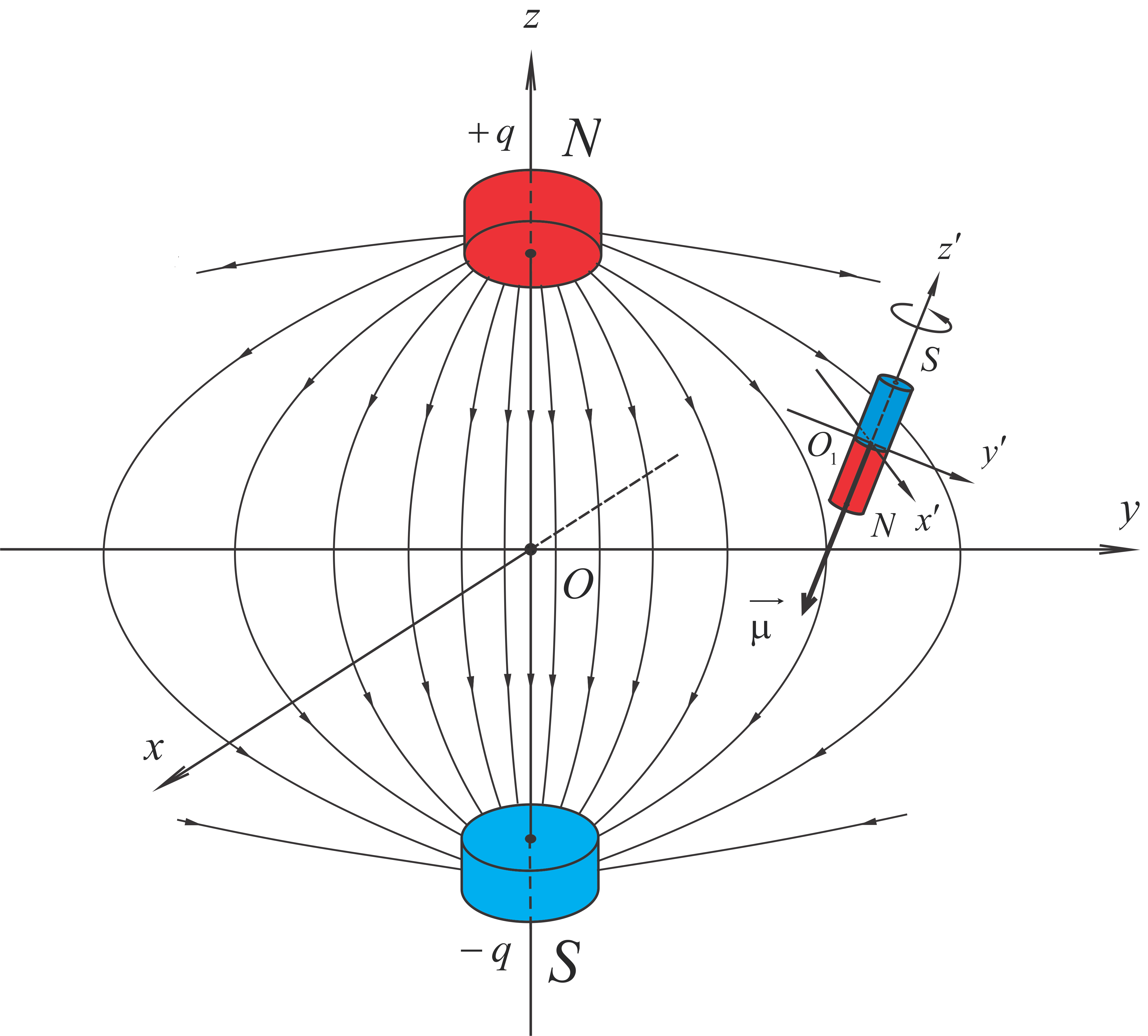
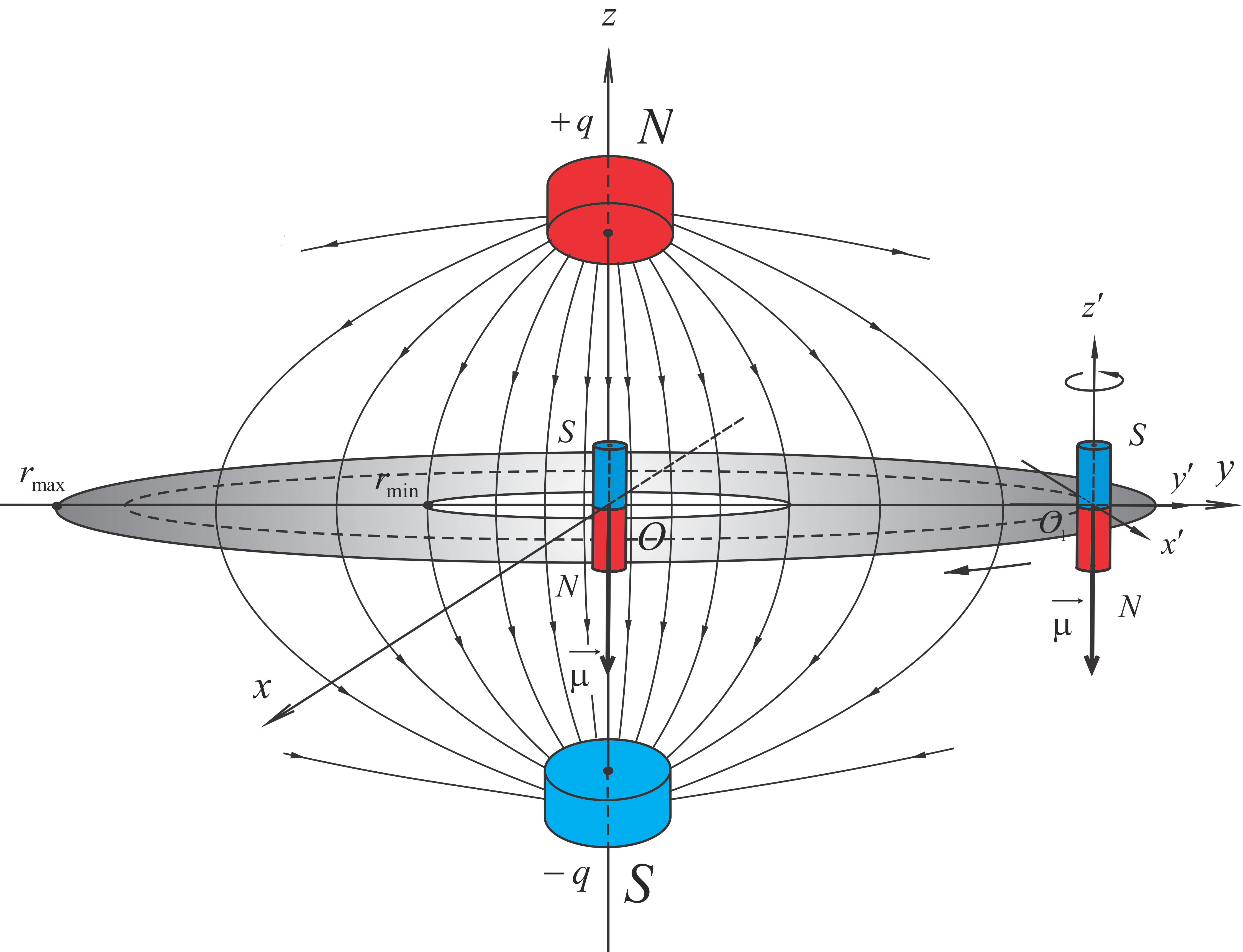
The standard orbitron is a a small axisymmetric magnetized rigid body (for example a small permanent magnet or a current-carrying loop) with magnetic moment , in the permanent magnetic field created by two fixed magnetic poles modeled by opposite charges placed at distance [Smy39] in the absence of gravity (see Figure 1); in this definition the adjective “small” refers to the size of the body in comparison with the distance between the magnetic poles. In this section we provide the Hamiltonian description of this physical system.
Phase space. The configuration space of the orbitron is the special Euclidean group in three dimensions . The factor of accounts for the position of the center of mass in space of the rigid body and specifies its orientation with respect to a fixed initial frame. The orbitron is a simple mechanical system in the sense that its Hamiltonian function is of the form kinetic plus potential energy and that its phase space is the cotangent bundle of its configuration space endowed with the canonical symplectic structure obtained as minus the differential of the corresponding Liouville one form.
As the cotangent bundle of any Lie group, can be right or left trivialized in order to obtain the so called space or body coordinates, respectively (see Appendix 5.1), of the phase space. These trivializations provide an identification of the bundle with the product , where the symbol stands for the dual of the Lie algebra of .
In this paper we will work in body coordinates unless it is specified otherwise. Using this representation, we denote by the elements of and by those of using body coordinates.
Equations of motion. The Hamiltonian of the orbitron is given by the sum of the kinetic and the potential energy, that is,
| (2.1) |
The expression of the kinetic energy is:
| (2.2) |
where is the mass of the axisymmetric magnetic body and the reference inertia tensor . The coincidence between the first two principal moments of inertia is related to an axial symmetry with respect to the third coordinate that we assume in the body. The potential energy is given by
| (2.3) |
where , is the magnetic moment of the axisymmetric rigid body/dipole, and is the strength of the magnetic field created by two magnetic poles/“charges” placed at the points and , , that is,
| (2.4) |
with , , and the magnetic permeability of vacuum. A small axisymmetric magnetized rigid body subjected to a external magnetic field of the form specified in (2.4) will be called a standard orbitron.
As we will see later on, most of the results that we present in this paper hold for systems with external magnetic fields that share the following symmetry properties presented by in (2.4), namely:
- (i)
-
Equivariance with respect to rotations around the axis:
(2.5) - (ii)
-
Behavior with respect to the mirror transformation
(2.6) according to the prescription
(2.7) (2.8) (2.9)
Consider an arbitrary magnetic field in the magnetostatic approximation in a domain free of other magnetic sources that satisfies these symmetry properties. A small axisymmetric magnetized rigid body subjected to the influence of such an external field will be called a generalized orbitron. The generic term orbitron will refer simultaneously to both the standard and the generalized orbitrons.
The equations of motion of the orbitron are determined by Hamilton’s equations:
| (2.10) |
where denotes the interior derivative, is Cartan’s exterior derivative, and the Hamiltonian vector field associated to . It can be proved (see Appendix 5.2) that in body coordinates, Hamilton’s equations (2.10) amount to the set of differential equations:
| (2.11) | |||
| (2.12) | |||
| (2.13) | |||
| (2.14) |
The symbol stands for the antisymmetric matrix associated to the vector via the Lie algebra isomorphism introduced in Appendix 5.1 and for the differential.
Toral symmetry of the orbitron and associated momentum map. The axial symmetry of the magnetic rigid body and the rotational spatial symmetry of the magnetic field created by the two poles with respect to rotations around the OZ axis endow this system with a toral symmetry which is obtained as the cotangent lift of the following action on the configuration space:
| (2.15) |
where denotes the rotation matrix around the third axis by an angle . The first circle action involving implies a spatial rotation of the center of mass of the body and the second one, given by , accounts for a rotation of the magnetic body around its symmetry axis. In Appendix 5.3 we show that the cotangent lift, also denoted by , is a canonical symmetry given by
| (2.16) |
that has an invariant momentum map associated given by:
| (2.17) |
A straightforward computation shows that the Hamiltonian of the orbitron is invariant with respect to the action (2.16), that is,
which, by Noether’s Theorem [AM78, Theorem 4.2.2], allows us to conclude that the level sets of the momentum map (2.17) are preserved by the associated Hamiltonian dynamics, that is, if is the flow of the vector field then for any .
The action (2.16) has two isotropy subgroups, namely, the identity and the diagonal circle . The orbit type submanifold is given by
| (2.18) |
and . The bifurcation lemma (see for instance [OR04, Proposition 4.5.12]) guarantees that the restriction of the momentum map to the regular isotropy type is a submersion and that it has rank one at points in the isotropy type .
3 Relative equilibria of the orbitron
In this section we specify the equations that characterize the relative equilibria of the orbitron with respect to its toral symmetry.
Relative equilibria: setup and background. Consider a vector field on a manifold that is equivariant with respect to action of a Lie group on it. We say that the point is a relative equilibrium with velocity if the value of vector field at that point coincides with the infinitesimal generator associated to , that is,
| (3.1) |
The Lie algebra element is called the velocity of the relative equilibrium. This defining property is equivalent to saying that the flow associated to the vector field at the point coincides with the one-parameter Lie subgroup of generated by , that is,
| (3.2) |
where is the Lie group exponential map . In the Hamiltonian setup, relative equilibria have a very convenient characterization that uses the critical points of a function instead of the equilibria of the vector field , as in (3.1). Indeed, consider now a symmetric Hamiltonian system and assume that the momentum map is coadjoint equivariant; it can be shown [AM78] that the point is a relative equilibrium of the Hamiltonian vector field with velocity if and only if
| (3.3) |
where . The combination is usually referred to as the augmented Hamiltonian. If the relative equilibrium is such that and we denote its isotropy subgroup with respect to the action by , the law of conservation of the isotropy [OR04] and Noether’s Theorem imply [OR99b, Theorem 2.8] that , where is the coadjoint isotropy of and is the normalizer group of in (note that necessarily due to the equivariance of the momentum map). Finally, notice that the velocity of a relative equilibrium with nontrivial isotropy is not uniquely defined; indeed, it is clear in (3.2) that if is a velocity for the relative equilibrium , then so is for any .
Relative equilibria equations of the orbitron. The next proposition, proved in Appendix 5.4, specifies the critical point equations (3.3) in the case of the orbitron and shows the existence of branches of relative equilibria whose stability we will study in the next section.
Proposition 3.1
Consider the orbitron system introduced in Section 2 whose Hamiltonian function is given by (2.1) and let . Then:
- (i)
-
The point is a relative equilibrium of the orbitron with velocity with respect to the toral symmetry introduced in Section 2 if and only if the following identities are satisfied:
(3.4) (3.5) (3.6) (3.7) - (ii)
-
Consider now , , and . The point is a relative equilibrium of the standard orbitron with velocity , where is an arbitrary real number and is either arbitrary when or
(3.8) when . In view of the expression (3.8) for the spatial velocity , the existence of the latter relative equilibrium is only guaranteed when .
- (iii)
-
The conclusions in the previous part also hold for the generalized orbitron. In this situation for some , and the spatial velocity of the relative equilibria with is given by
(3.9) where . In view of the expression of the spatial velocity in (3.9), the existence of this relative equilibrium is only guaranteed when .
The relative equilibria in these statements for which (respectively ) have trivial (respectively nontrivial ) isotropy and hence belong to the orbit type (respectively ); we will refer to them as regular relative equilibria (respectively singular relative equilibria).
4 Stability analysis of the relative equilibria of the orbitron
In this section we study the stability properties of the branches of relative equilibria of the orbitron introduced in the second and third parts of Proposition 3.1.
The energy–momentum method. As we already explained in the introduction, the degeneracies present in symmetric systems cause various drift phenomena that complicate the selection of a stability criterion. The most natural and fruitful choice is that of stability relative to a subgroup, introduced in [Pat92] for relative equilibria and in [OR99a] for relative periodic orbits.
Definition 4.1
Let be a –equivariant vector field on the –manifold and let be a subgroup of . A relative equilibrium of , is called –stable, or stable modulo , if for any –invariant open neighborhood of the orbit , there is an open neighborhood of , such that if is the flow of the vector field and , then for all .
In the Hamiltonian setup there exists a variety of Dirichlet type results that provide sufficient conditions for the –stability of a given relative equilibrium, where is the momentum value in which it is sitting and is its coadjoint isotropy. The reason why the subgroup arises naturally is clear if we look at the stability problem from the symplectic reduction point of view; more explicitly, consider a symmetric Hamiltonian system that exhibits a relative equilibrium at the point such that . Suppose that the momentum map is coadjoint equivariant and that the coadjoint isotropy acts freely and properly on the momentum fiber ; in these conditions, the quotient space is naturally symplectic [Mey73, MW74] and the -equivariant Hamiltonian vector field associated to projects onto another Hamiltonian vector field in which the relative equilibrium becomes a standard equilibrium. The importance of this construction in our context comes from the fact that the standard Lyapunov stability of the reduced equilibrium is equivalent to the –stability of the relative equilibrium.
The following result, known as the energy–momentum method, provides a sufficient condition for the –stability of a given relative equilibrium. This result has been introduced at different levels of generality in [Pat92, OR99b, PRW04, MRO11].
Theorem 4.2 (Energy-momentum method)
Let be a symplectic Hamiltonian system with a symmetry given by the Lie group acting properly on with an associated coadjoint equivariant momentum map . Let be a relative equilibrium such that and assume that the coadjoint isotropy subgroup is compact. Let be a velocity of the relative equilibrium. If the quadratic form
| (4.1) |
is definite for some (and hence for any) subspace such that
then is a –stable relative equilibrium. If , then is always a –stable relative equilibrium. The quadratic form , will be called the stability form of the relative equilibrium and a stability space.
Remark 4.3
Remark 4.4
The statement in Theorem 4.2 can be generalized to the context of Hamiltonian actions on Poisson manifolds and can be stated so that one can take advantage of existing Casimirs or other non-symmetry related conserved quantities in order to prove the stability of a given relative equilibrium [OR99c, Theorem 4.8]. More explicitly, if in the conditions of Theorem 4.2 there exists a set of –invariant conserved quantities for which
and
is definite for some (and hence for any) such that
then is a –stable relative equilibrium.
Nonlinear stability of the orbitron relative equilibria. The application of the energy-momentum method to the relative equilibria of the orbitron introduced in Proposition 3.1 makes possible the determination of sizeable regions in parameter space for which those solutions are -stable (-stable in this case). We spell this out in the statement of the following theorem whose proof is provided in the Appendix 5.5.
Theorem 4.5
Consider the relative equilibria introduced in Proposition 3.1. Then:
- (i)
-
The regular relative equilibria of the standard orbitron in part (ii) of Proposition 3.1, that is, those for which , are –stable whenever the following three inequalities are satisfied:
(4.2) (4.3) where , , and .
The singular relative equilibria () are always formally unstable, in the sense that the stability form (4.1) exhibits a nontrivial signature.
- (ii)
-
The regular relative equilibria of the generalized orbitron in part (iii) of Proposition 3.1 are –stable whenever the following conditions hold:
(4.4) (4.5) (4.6) (4.7) where , is the function such that , , , , , and .
The singular branch () is –stable if the following conditions are satisfied:
(4.8) (4.9) (4.10) (4.11) where and we use the same notation as above for , , and , replacing by . When and , the conditions (4.10) and (4.11) can be replaced by the following single –independent optimal condition:
(4.12) This optimal condition is achieved by using the spatial velocities ; the positive (respectively negative) sign for the velocity corresponds to positive (respectively negative) values of .
Remark 4.6
The right inequality in (4.2) was already known by Kozorez [Koz81] but it does not ensure by itself the nonlinear stability of this symmetric configuration. We will refer to this inequality as the Kozorez condition. The extension of this inequality in the context of the generalized orbitron is given by (4.5).
Remark 4.7
The formal instability of the singular branch of the standard orbitron is not informative about its actual nonlinear stability or instability. This point is determined via a complementary spectral stability analysis of the linearized system that we carry out later on in Theorem 4.13 and that allows us to conclude the nonlinear instability of this singular branch of relative equilibria.
Remark 4.8
The proof of the theorem presented in Appendix 5.5 consists of studying the definiteness of the stability form (4.1) introduced in Theorem 4.2. A quick dimension count shows that the stability spaces corresponding to the regular and singular branches of relative equilibria are eight and ten dimensional, respectively. The need of determining the sign of the eigenvalues of stability forms in high dimensions like ours has motivated the introduction in the literature of various block diagonalizations for it based on arguments of dynamic [SLM91, RO06] or kinematic [OR99b] nature. An elementary but important observation that we point out in the proof of this theorem is that in order to ensure the stability of the relative equilibrium in question there is no need to compute the eigenvalues of the stability form but only to determine its signature; the relevance of this statement lies in the fact that by Sylvester’s Law of Inertia, the signature is invariant by conjugation with respect to invertible matrices and hence can be read out of the pivots of the matrix obtained by performing Gaussian elimination on the stability form. Unlike the situation faced when computing eigenvalues, Gaussian elimination can be carried out formally and not just numerically in virtually any dimension. This remark is of much importance for non-simple mechanical systems for which dynamic block diagonalizations similar to those cited above are rarely available.
Remark 4.9
Conditions (4.8)–(4.11) can be used in the design of magnetic fields capable of confining magnetic rigid bodies that do not exhibit spatial rotation. This is the working principle of devices such as magnetic contactless flywheels or levitrons. In the case of flywheels, up until now only actively controlled versions have been developed; as to the levitron, the potentials that have been considered so far [DE99, Dul04, KM06] do not allow to conclude nonlinear stability using the methods put at work in Theorem 4.5 and only the spectral stability of the corresponding linearized systems has been considered. We plan to explore in detail these systems in a future publication.
Linear stability and instability analysis tools for relative equilibria. The use of the energy-momentum method provides sufficient but not necessary nonlinear stability conditions. More specifically, there is no guarantee that the stability regions determined by the inequalities in the statement of Theorem 4.5 are optimal in the sense that as soon as those conditions are violated stability disappears. In the context of stability studies for standard equilibria one usually proceeds by examining the spectral stability of the linearization at the equilibrium of the vector field in question, that is, when the sufficient stability conditions obtained via a Dirichlet type criterion are violated, one looks for eigenvalues of the linearization that exhibit a nonzero real part, whose existence would imply the nonlinear instability of the equilibrium of the original vector field.
This way to proceed can be extended in the context of regular relative equilibria by looking at the spectral stability of the linearization of the reduced Hamiltonian vector field at the equilibrium corresponding to the relative equilibrium in the symplectic Marsden–Weinstein reduced space [MW74]. Even though in the singular case, there exist reduced spaces that generalize the Marsden–Weinstein reduced space [SL91, OR06a, OR06b], the equivalence between -stability of a relative equilibrium and standard nonlinear stability of the corresponding reduced equilibrium does not hold anymore, which makes necessary the formulation of a criterion that, as the energy-momentum method in Theorem 4.2, provides a linear stability analysis tool for relative equilibria whose formulation does not need reduction; such a statement is provided in the next proposition, whose proof can be found in the appendix, and we will apply it later on to the branches introduced in Proposition 3.1 whose nonlinear stability was studied in Theorem 4.5. In order to fix the notation and to make the presentation self contained, we start by recalling the notion of linearization of a vector field at an equilibrium point.
Definition 4.10
Let be a vector field on the manifold and let be an equilibrium point, that is, . The linearization of at the point is a vector field on the vector space , defined by
where is the flow of . The eigenvalues of the linear map are called the characteristic exponents of at . The map is the projection onto the second factor.
Proposition 4.11
Let be a Lie group acting canonically and properly on the symplectic manifold and suppose that there exists a coadjoint equivariant momentum map that can be associated to it. Let be a –invariant Hamiltonian and let be a relative equilibrium of the corresponding –equivariant Hamiltonian vector field with velocity . Consider a –invariant stability space such that
with and the coadjoint isotropy of . Then:
- (i)
-
with is a symplectic vector subspace of .
- (ii)
-
There exists a symplectic slice at such that .
- (iii)
-
The Hamiltonian vector field in associated to the Hamiltonian function exhibits an equilibrium at the point .
- (iv)
-
The linearization of at coincides with the linear Hamiltonian vector field on that has as Hamiltonian vector field the stability form
- (v)
-
Suppose that the two tangent spaces and coincide. Then
(4.13) Additionally, let be the augmented Hamiltonian and let be the linearization of the Hamiltonian vector field at . Then
(4.14) where is the inclusion, is the projection according to (4.13), and is the linearization of at .
- (vi)
-
If the linear vector field is spectrally unstable in the sense that it exhibits eigenvalues with a nontrivial real part, then the relative equilibrium of is nonlinearly –unstable, for any subgroup .
We now provide a result that spells out how to compute the linearization of a Hamiltonian vector field at an equilibrium for systems whose phase space is the cotangent bundle of a Lie group. The following proposition expresses the linearization that we need in terms of a linear map on the Euclidean vector space formed by the direct product of the Lie algebra and its dual.
Proposition 4.12
Let be a Lie group with Lie algebra and let be its cotangent bundle endowed with the canonical symplectic form. Consider now the body coordinates (left trivialized) expression of and let be a Hamiltonian function whose associated Hamiltonian vector field exhibits an equilibrium at the point . Then:
- (i)
-
Let be the cotangent lift of the action by left translations of on expressed in body coordinates. Let ; the Hamiltonian vector field exhibits an equilibrium at the point .
- (ii)
-
Let and let (respectively be the quadratic form associated to the second derivative of at (respectively of at ). Then
(4.15) and the associated linear Hamiltonian vector fields considered as linear maps satisfy:
(4.16) - (iii)
-
The linearization is given by:
(4.17) where , are the canonical projections and is the linear map associated to the Hessian of at by the relation
We now implement the expression for the linearization of a Hamiltonian vector field obtained in this proposition, in the particular case of the cotangent bundle . Let be a Hamiltonian function and let be the corresponding Hamiltonian vector field that we assume has an equilibrium at the point , that is, . Let and let ; using the notation in the previous proposition, it is clear that . Let be the linear map associated to the Hessian of at , that is, for any ,
Now, given , define the projection (also available also for the , , components):
| (4.18) |
By relations (4.16) and (4.17) in Proposition 4.12, and the expression (5.10), the linearization of at is given by
| (4.19) |
where is the linear map determined by the twelve by twelve matrix
| (4.20) |
This expression should be understood as a vertical concatenation of four matrices with three rows and twelve columns each. More explicitly, given that for any , , we can write
where is the image by (4.20) of the vector .
Linear stability and instability of the orbitron relative equilibria. The results presented in the previous paragraph provide all the necessary tools to carry out the linear stability analysis of the relative equilibria of the standard and generalized orbitron introduced in the parts (ii) and (iii) of Proposition 3.1. We will proceed by using expressions (4.19) and (4.20) in order to compute the linearization at the relative equilibria of the Hamiltonian vector fields associated to the augmented Hamiltonians constructed with the appropriate relative equilibrium velocities. We subsequently use part (v) of Proposition 4.11 in order to write down the linearization of the restriction of this vector field to the tangent space to a symplectic slice (equivalently, a stability space); finally, we use the last part of this result in order to search for instability regions by looking for eigenvalues of this linearization that exhibit a nontrivial real part and determine how sharp the nonlinear sufficient stability conditions in Theorem 4.5 are; more specifically, we will see that there might exist relative equilibria that are nonlinearly stable even though the conditions in Theorem 4.5 are not satisfied. A detailed description of this implementation is provided in Appendix 5.7. The following result, formulated using the terminology introduced in Proposition 3.1, summarizes the results of the linear analysis.
Theorem 4.13
Consider the relative equilibria introduced in Proposition 3.1. Then:
- (i)
-
Regarding the relative equilibria of the standard orbitron in part (ii) of the proposition:
- (a)
-
The regular relative equilibria that do not satisfy the Kozorez relation () are unstable and this stability condition is consequently sharp. The other two stability conditions in (4.2) and (4.3) are not sharp, that is, there are regions in parameter space that do not satisfy them and where the linearized system is spectrally stable.
- (b)
-
The singular relative equilibria of the standard orbitron are nonlinearly unstable.
- (ii)
-
Regarding the relative equilibria of the generalized orbitron in part (iii) of the proposition:
- (a)
-
The regular relative equilibria that do not satisfy the generalized Kozorez relation (4.5), namely, , are unstable and this stability condition is consequently sharp. The remaining stability conditions (4.4), (4.6), and (4.7) are not sharp, that is, there are regions in parameter space that do not satisfy them and where the linearized system is spectrally stable.
- (b)
Proof. (i) Part (a) The linearization at the regular relative equilibria of the Hamiltonian vector field in the stability space associated to the augmented Hamiltonian is provided in the expression (5.95). This matrix is block diagonal and the top two by two block has as eigenvalues
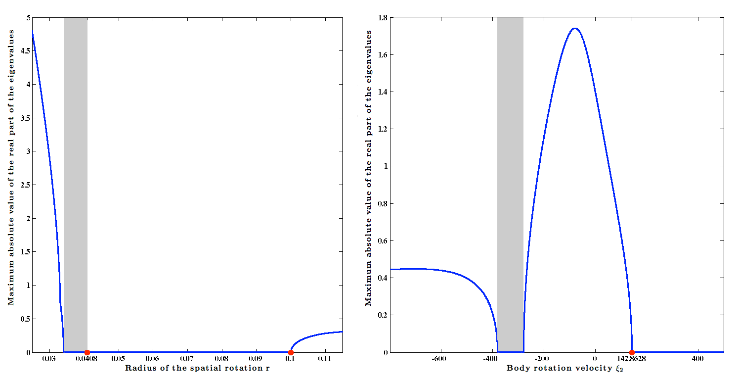
which are real whenever , that is, when the Kozorez relation is violated. In conclusion, the part (vi) of Proposition 4.11 ensures that as soon as the Kozorez relation is violated the relative equilibria cease to be stable. The lack of sharpness of the two other stability conditions in (4.2) and (4.3) is observed by studying the spectrum of the remaining six by six block of the linearization which may be purely imaginary in regions of the parameter space in which those conditions are violated. The expressions corresponding to those six eigenvalues are very convoluted and we therefore do not include them in the paper; in turn, we illustrate this phenomenon in Figure 3, in which we plot the maximum absolute value of the real part of the eigenvalues of the linearization versus the radius of spatial rotation and the body rotation velocity , respectively, when all the system parameters specified in the caption remain constant. The graph on the left hand side shows that when the radius goes beyond the critical value stipulated by the left inequality in (4.2) the spectrum of the linearization remains purely imaginary for a while and the system is hence potentially stable; it is also visible that, as we proved above, the system becomes spectrally unstable as soon as the Kozorez relation ceases to be satisfied. The lack of sharpness of the condition (4.3) is illustrated in the right hand side graph and is of a slight different nature; indeed, as soon as the condition is not satisfied, spectral instability appears but if the body rotation velocity is sufficiently decreased the system becomes again spectrally stable in some interval of the parameter space.
(i) Part (b) The corresponding linearization at the singular relative equilibria is described in (5.96). Its spectrum includes the two following eigenvalues:
The eigenvalue can only be purely imaginary when . This in turns implies that the term in is purely imaginary and prevents the eigenvalue to be purely imaginary unless is zero.
(ii) Part (a) Analogously to the situation in the proof of (i) Part (a), the linearization at the regular relative equilibria of the generalized orbitron exhibits the following two eigenvalues:
which are obviously purely imaginary if and only if the generalized Kozorez relation (4.5) holds. The lack of sharpness in the remaining relations follows from the fact that they contain as particular cases the stability conditions for the standard orbitron that, as we illustrated in Figure 3, are not necessary for the spectral stability of .
(ii) Part (b) The linearization at the singular relative equilibria of the generalized orbitron is provided in (5.97) and its spectrum is made up by the following ten eigenvalues:
| (4.24) | ||||
| (4.25) | ||||
| (4.26) |
The eigenvalues can be purely imaginary only when . In order for the four eigenvalues to have the same property, the term has to be necessarily a real number, which yields the condition . These two relations obviously imply that the nonlinear stability conditions (4.8) and (4.9) are sharp. Finally, the remaining four eigenvalues are purely imaginary whenever the term is real, which requires in turn that the relation is satisfied. We note that this relation may hold without (4.10) and (4.11) or (4.12) being satisfied. Indeed, take for example a system for which ; in that situation, the relation (4.23) does not impose any constraint on an hence it is easy to find values for this variable that violate (4.10) and (4.11) or (4.12).
5 Appendices
5.1 The geometry of the phase space of the orbitron
Lie group and Lie algebra structure of the configuration space. The configuration space of the orbitron is the Lie group endowed with the semidirect product structure associated to the composition rule
| (5.1) |
for which and . In order to spell out the Lie algebra structure associated to the Lie product (5.1) we start by recalling the Lie algebra isomorphism between the Lie algebra of and endowed with the standard cross product, given by the assignment
We recall that isomorphism satisfies that and that for any and
| (5.2) | |||
| (5.3) | |||
| (5.4) |
where (respectively ) denotes left (respectively right) translations and is the adjoint representation. The isomorphism induces another one
uniquely determined by the relation , with the Euclidean inner product in . Using this isomorphism, we have
| (5.5) |
Using this notation, the Lie algebra structure of is given by the bracket
| (5.6) |
Additionally, for any , , , , the following relations that we use later on in the paper hold
| (5.7) | ||||
| (5.8) | ||||
| (5.9) | ||||
| (5.10) | ||||
| (5.11) | ||||
| (5.12) |
In the last two expressions we have identified with using the Frobenius norm in the part and the Euclidean norm in the part. Using these equalities, it is easy to see that the adjoint and coadjoint actions of on its algebra and its dual are determined by:
| (5.13) | ||||
| (5.14) |
Body and space coordinates for . Given an arbitrary Lie group with Lie algebra , we recall (see for example [AM78]) that the maps
| (5.15) |
define trivializations of the tangent and cotangent bundles , respectively, that are usually referred to as space coordinates of these bundles. Notice that if , , then .
Analogously, the trivializations obtained using left translations instead via the maps
| (5.16) |
are usually referred to as body coordinates. Notice that if , , then .
5.2 Equations of motion of the orbitron
In this section we obtain the equations of motion (2.11)-(2.14) of the orbitron using body coordinates. We will proceed by writing down first the differential equations that define a Hamiltonian vector field on the left trivialized cotangent bundle of an arbitrary Lie group with Lie algebra .
Proposition 5.1
Let be a Lie group with Lie algebra and let be its cotangent bundle endowed with the canonical symplectic form. Let be the corresponding symplectic form on the trivial bundle obtained out of by left trivialization (body coordinates) and let be a Hamiltonian function. For any , the Hamiltonian vector field associated to is given by
| (5.19) |
where and are determined by
| (5.20) | |||||
| (5.21) |
Proof. Using the expression of the canonical symplectic form of in body coordinates (see for instance [OR04, Expression (6.2.5)]) it is easy to see that , , and hence , are determined by the relation
where and are arbitrary and and are the partial derivatives of with respect to and , respectively. Equivalently,
as required.
We now consider the case we are interested in, that is, and
| (5.22) |
Let
be an arbitrary element of and . Then, as
we can conclude that
| (5.25) | ||||
| (5.28) |
Now using (5.20) and (5.21), together with and (5.25), (5.28), (5.10), and (5.12), we obtain
Consequently, by (5.19) we conclude that the equations of motion associated to the Hamiltonian (5.22) are
5.3 The toral action on phase space and the associated momentum map
The expression of the lifted action in body coordinates. We start by proving that the cotangent lift of the toral action on in (2.15) is given by (2.16) when using body coordinates. Consider and two arbitrary Lie groups and let be an action of on . We recall that the lift of this action to the cotangent bundle of , also denoted by , is given by
Using the maps introduced in (5.16), this action is expressed in body coordinates as:
or equivalently,
In the particular case of , , and the toral action introduced in (2.15), that is,
we consider , , and . Then,
| (5.29) |
In order to compute the second part of this expression let . Then
Given that by (5.4) , the last equality together with (5.29) yield the expression (2.16) of the lifted action in body coordinates, that is,
| (5.30) |
The infinitesimal generators of the toral action. We first show that for any Lie algebra element and ,
| (5.31) | ||||
| (5.32) |
We start by proving the first equality
where in the last equality we used (5.8). Regarding (5.32), note that
where we used (5.7).
The infinitesimal generator of the lifted -action on in body coordinates is given by
| (5.33) |
Indeed,
The momentum map of the toral action Given a lifted action of a Lie group on the cotangent bundle of a Lie group endowed with the canonical symplectic form, the map defined by
| (5.34) |
is a coadjoint equivariant momentum map for this canonical action (see [AM78, Corollary 4.2.11]). We now study the particular case we are interested in, that is, , , and consider an arbitrary point , and the covector that in body coordinates is expressed as . With this notation, the expression in body coordinates of the momentum map in (5.34) is given by
| (5.35) |
Indeed, for any ,
which proves (5.35) since is arbitrary.
5.4 Proof of Proposition 3.1
(i) Using the statement preceeding (3.3) we will specify the relative equilibria of the orbitron by characterizing the points for which
| (5.36) |
for some . We start by computing the tangent of the momentum map and the differential of the Hamiltonian. Let be an arbitrary vector at the point , then it is easy to check that
| (5.37) | ||||
| (5.38) |
with and the kinetic and potential energies introduced in (2.2). Additionally,
| (5.39) |
Consequently, using (5.37), (5.38) and (5.39) we have, for any
| (5.40) |
Therefore, as , , , and in this expression are arbitrary, it can be checked that the points for which are characterized by the equations:
| (5.41) | ||||
| (5.42) | ||||
| (5.43) | ||||
| (5.44) |
as required.
(ii) We show that the points of the form specified in the statement of the proposition satisfy equations (5.41)–(5.44) and hence constitute a branch of relative equilibria. We proceed by considering and and using equations (5.41)–(5.44) to determine , , and the velocity in the statement.
Notice first that , hence by (5.44) we have that
| (5.45) |
necessarily. Now by (5.43)
| (5.46) |
In order to handle (5.42) we note that is given by the matrix whose components are
where , and . Consequently,
where . Hence
| (5.47) |
Note additionally that by (5.45)
| (5.48) |
Then by equalities (5.47) and by (5.48), equation (5.42) holds whenever or when and ; we note that in both situations, there are no restrictions on the second component of the velocity . Finally, it can be readily verified that (5.41) always holds at the point by using that .
(iii) Suppose that we are in the presence of a magnetic field equivariant with respect to rotations around the axis and that behaves as indicated in (2.7)–(2.9) with respect to the mirror transformation (2.6). Notice first that by (2.7) and (2.8)
| (5.49) |
and hence
| (5.50) |
Additionally, by (2.5), is rotationally invariant with respect to rotations in the plane, hence
| (5.51) |
Conditions (3.7) and (3.6) show that if and , then and necessarily. If we use and (5.50) in the expression (3.4), it can be easily verified that this relation is automatically satisfied.
5.5 Proof of Theorem 4.5
We will proceed by using Theorem 4.2 in order to determine the regions in parameter space for which the stability form (4.1) at the relative equilibria is definite, which in turn ensures –stability.
We start by denoting the augmented Hamiltonian as , for any . Let expressed in body coordinates. As we saw in the proof of Proposition 3.1 (see Appendix 5.4), the partial derivatives of are given by:
-
•
,
-
•
,
-
•
,
-
•
.
In order to compute the Hessian of the augmented Hamiltonian, we write down the derivatives of its partial derivatives in the direction given by the vector . A straightforward computation yields:
-
•
,
-
•
, where
-
•
,
-
•
.
Consequently, the matrix expression associated to is given by:
| (5.54) |
We now compute the value of the Hessian (5.54) at the relative equilibria in the second and third parts of Proposition 3.1, that is, with , , , and . We start by noticing that
| (5.55) |
Indeed, for any
| (5.56) |
Therefore, the matrix expression associated to is given by:
| (5.57) |
In order to construct stability forms for the regular and singular branches, we now determine stability spaces to which we will restrict the Hessian (5.57).
A stability space for the regular branch (). In this case, the kernel of the derivative of the momentum map is given by:
and using (5.33), the tangent space to the toral orbit that goes through the relative equilibrium can be characterized as:
Finally, it can be easily verified that the vector subspace
is such that
| (5.58) |
and hence constitutes a stability space. Moreover, let , , , , , , , and . It can be checked that
| (5.59) |
The set will be used as a basis of the stability space in order to obtain matrix expressions for the stability form corresponding to each part of Theorem 4.5.
A stability space for the singular branch (). Consider now the relative equlibrium with , , , and , . In this case, the matrix expression (5.54) associated to is given by:
| (5.60) |
These relative equilibria lay on the singular isotropy type manifold (2.18) and hence by the Bifurcation Lemma (see [OR04, Proposition 4.5.12]), the kernel of the derivative of the momentum map is necessarily of dimension eleven at those points. Indeed, it can be checked that:
and using (5.33), the tangent space to the toral orbit that goes through the singular relative equilibrium can be characterized as:
Finally, it can be easily verified that the vector subspace given by
| (5.61) |
with , , , , , , , , , and is a –invariant stability space, that is,
| (5.62) |
and hence constitutes a stability space. We recall that is the isotropy subgroup of the relative equilibrium . We will use the set as a basis of the stability space in order to obtain a matrix expression for the stability form for the parts (i) and (ii) of Theorem 4.5.
Proof of part (i) of the theorem.
Stability study for the regular branch. We start by noting that the stability of a relative equilibrium can be determined by using any of the the points that constitute its trajectory in phase space. Hence we can, without loss of generality, use the relative equilibrium point of the form . We recall that the regular relative equilibria are those for which and
We now provide the expression of using the same notation as in (5.47) and conclude that
By (5.57) and (5.59) we obtain that the stability form can be written as:
| (5.63) |
where . Notice that this matrix is block diagonal and exhibits two blocks of size two and six. The positivity of the block of size two requires that and . The first inequality is always satisfied when and the second one amounts to
| (5.64) |
which yields the right hand side inequality in (4.2). We now study the positivity of the lower six dimensional block of the stability form. As we already pointed out in Remark 4.8, given that by Sylvester’s Law of Inertia the signature of a diagonalizable matrix is invariant with respect to conjugation by invertible matrices, it can hence be read out of the pivots of the matrix obtained by performing Gaussian elimination on this block. Indeed, these pivots are
| (5.65) |
where
The first three are automatically positive. The positivity of is equivalent to
which yields the left hand side inequality in (4.2) Finally, we study the positivity of the last two pivots and . The simultaneous positivity of and is equivalent to . It is easy to check that , since the condition
| (5.66) |
is always satisfied due to (5.5) and the condition . Regarding the positivity of there are two possible cases:
1)
, then
2) , then
and hence the positivity of can be summarized as
which coincides with (4.3), as required.
Stability study for the singular branch. We first notice that the matrix expression associated to is given by (5.60), where
| (5.67) |
Consequently, the pivots obtained by Gaussian elimination in the matrix expression of the stability form are
| (5.68) |
where
The formal instability of the singular branch is caused by the fact that the pivots in (5.68) cannot simultaneously have all the same sign. Indeed, and are always positive which forces . This is in turn incompatible with because that would require , which is not possible.
Proof of part (ii) of the theorem.
Stability study for the regular branch. In order to prove the second part of Theorem 4.5, we follow the same pattern that we used above. Let be the function such that and . Additionally,
and we recall that . We now compute the components of the matrix . Using the equations (5.49), (5.52) and (5.51) we obtain
In order to determine the remaining two components in , we use the Ampère-Maxwell equation in the absence of additional currents and time-varying electric fields in the region where the body motion takes place. Indeed, implies that
and hence,
By expression (5.55)
| (5.69) |
Using the same argument as in the proof of part (i) we use, without loss of generality, the relative equilibrium point of the form , , where . The matrix expression of is:
| (5.70) |
where . Notice that this matrix is block diagonal and exhibits two blocks of size two and six. The positivity of the block of size two requires that and which coincide with (4.4) and (4.5). We now study the positivity of the lower six dimensional block of the stability form. As we did in the proof of part (i), we will read the signature of this block out of its pivots, which are , , , , , and . The first three are automatically positive. The positivity of the fourth requires
| (5.71) |
which corresponds to the inequality (4.6) in the statement. Finally, we study the positivity of the last two pivots. Let
| (5.72) |
and
| (5.73) |
The simultaneous positivity of and is equivalent to . It is easy to check that , since the condition
| (5.74) |
is satisfied due to (5.71). The positivity of can be summarized as
which coincides with (4.7), as required.
Stability study for the singular branch. The matrix expression associated to is given by (5.60), where in this case
| (5.75) |
The pivots obtained by Gaussian elimination in the matrix expression of the stability form are
where
The pivots and are automatically positive. The positivity of the pivots , , and requires that:
| (5.76) | |||
| (5.77) | |||
| (5.78) | |||
| (5.79) |
which yields the conditions (4.9)–(4.11). We now derive the optimal stability condition (4.12). Let in (4.11). It is easy to verify that the function has a minimum at and a maximum at provided that . Since the condition (4.10) has to be satisfied, then also needs to hold. In that case, the choices and the inequalities
determine the largest possible stability region in the (and consequently the ) variable, as required in (4.12).
5.6 Proofs of Propositions 4.11 and 4.12
Proof of Proposition 4.11
(i) It is a consequence of the Witt-Artin decomposition (see for example [OR04, Theorem 7.1.1]).
(ii) It is a consequence of the fact that the symplectic slice introduced by Marle [Mar84, Mar85], Guillemin, and Sternberg [GS84] can be constructed by Riemannian exponentiation of a symplectic tube. Since we need this construction in the proof of the following parts of the proposition, we briefly recall it using the notation in Chapter 7 of [OR04].
The first step is the splitting of the Lie algebra of into three parts. The first summand is . The equivariance of the momentum map implies that and hence . Hence we can fix an -invariant inner product on (always available by the compactness of ) and write
| (5.80) |
where is the -orthogonal complement of in and is the -orthogonal complement of in . The splittings in (5.80) induce similar ones on the duals
| (5.81) |
Each of the spaces in this decomposition should be understood as the set of covectors in that can be written as , with in the corresponding subspace. For example, .
The second ingredient in the construction of the symplectic tube comes from noting that the compact (by the properness of the action) isotropy subgroup acts linearly and canonically on with momentum map given by
It can be shown [OR04, Proposition 7.2.2] that there exist –invariant neighborhoods and of the origin in and , respectively, such that the twisted product is endowed with a natural symplectic form whose expression can be found in (7.2.2) of [OR04]. The Lie group acts canonically on by , for any and , and has a momentum map associated given by the so called Marle–Guillemin–Sternberg normal form:
The –symplectic manifold is called a symplectic tube of at the point . This denomination is justified by the Symplectic Slice Theorem [Mar84, Mar85, GS84] that proves the existence of a –equivariant symplectomorphism between a –invariant neighborhood of in and satisfying . The symplectic slice in the statement of the proposition is obtained [OR04, Theorem 7.4.1] as , where and, more explicitly, as , with the Riemannian exponential associated to a –invariant metric. The identity is a consequence of the fact that .
(iii) Since is a relative equilibrium, we have . This implies that and hence .
(iv) This statement is a consequence of the combination of (ii) and (iii) with the following lemma.
Lemma 5.2
Let be a symplectic manifold, , and the corresponding Hamiltonian vector field. Suppose that is an equilibrium point of , that is and consequently . Then, the linearization of at is a Hamiltonian vector field on the symplectic vector space with Hamiltonian function given by
| (5.82) |
Proof of the Lemma. Note and . Let arbitrary and let be a curve such that . Then if is the flow of , we write
| (5.83) |
We now take a Darboux chart [AM78, page 75] around the point . Recall that in Darboux coordinates, the symplectic form is constant. Additionally if , let be such that . Now, since , then (5.83) can be written as
Consequently, , as required.
(v) The hypothesis implies that ; this fact and the construction of the Witt–Artin decomposition (see for example the expression (7.1.11) in [OR04]) ensure that (4.13) holds. In order to prove (4.14), notice that for any
where we used that and hence . Since are arbitrary, the equality implies that
which is equivalent to (4.14).
(vi) Given the local and group invariant character of this statement, we will prove this statement using the so called reconstruction differential equations [Ort98, RWL02, OR04] that determine the Hamiltonian vector field associated to a –invariant Hamiltonian in the symplectic tube . Consider first the orbit projection; the –invariance of implies that the composition can be understood as a –invariant function on that does not depend of the first factor, that is, . The reconstruction equations show that for any ,
where , , and are determined by the expressions
| (5.84) | |||||
| (5.85) | |||||
| (5.86) |
where is the projection according to the splitting (5.81) and is the isomorphism associated to the symplectic form in .
We now assume that is spectrally unstable, which implies by part (iv) that the Hamiltonian vector field on the symplectic slice exhibits an unstable equilibrium at . Notice now that the Hamiltonian vector field is given by the projection onto via of the vector field in determined by
where is the projection according to the splitting (5.80), is the infinitesimal generator associated to using the –action on , and is the vector field in (5.85) that determines the dynamics induced by on the space . The instability of at implies the same feature for at and hence the –instability of the relative equilibrium of , for any subgroup .
Proof of Proposition 4.12
(i) It is a straightforward consequence of the chain rule as implies that .
(ii) Relation (4.15) is a consequence of the following general fact about Hessians: let and , with and smooth manifolds and let be a smooth map such that . Let with . Then , that is, for any :
In order to establish relation (4.16) note that the map is a symplectomorphism and hence a Poisson map. Expression (4.16) follows from [OR04, Proposition 4.1.19].
(iii) By Lemma 5.2, the Hamiltonian vector field is determined by the relation or, more explicitly, by
Using the expression of the canonical symplectic form of in body coordinates (see for instance [OR04, Expression (6.2.5)]), this equality can be rewritten as
| (5.87) |
Let now and be the maps defined by and , for any , and and , the canonical injections. Since (5.87) holds for arbitrary, we apply it to vectors of the form and and we obtain the following two equalities
Since in these expressions are arbitrary, they can be rewritten as:
| (5.88) | |||||
| (5.89) |
We now apply and to both sides of (5.88) and (5.89), respectively, and we notice that , , , , , and . We obtain
| (5.90) | |||||
| (5.91) |
which is equivalent to (4.17).
5.7 Linear stability and instability of the standard and generalized orbitron relative equilibria
The linearization for the regular branches. The goal in this paragraph is determining the linear Hamiltonian vector fields in the stability space used in the proof of Theorem 4.5 by using the expression (4.14) in Proposition 4.11. Notice that this is indeed possible due to the Abelian character of our symmetry group that ensures that in this situation and hence the coincidence of the tangent spaces and that is necessary as a hypothesis in this statement. We start by writing down the decomposition (4.13) that in this case can be achieved by noting that
| (5.92) |
with . If we use as a basis for the vectors introduced in (5.59) and for the ones those that we just described, it is easy to see that the matrix expressions of the inclusion and the projection , where is endowed with the canonical basis, are given by
| (5.93) | |||||
| (5.94) |
where the apostrophes stand for the transposition operation and the vertical indicate matrix concatenation. The linearization of the Hamiltonian vector field associated to the augmented Hamiltonian at the relative equilibria of the standard orbitron can be immediately obtained by using the expression (4.20) together with the Hessian already computed in (5.54) in the context of the proof of Theorem 4.5. The resulting expression is inserted in (4.14) using the injection (5.93) and the projection (5.94) and yields the following matrix for :
| (5.95) |
where . An analog expression can be obtained for the linearization at the regular relative equilibria of the generalized orbitron:
The linearization for the singular branches. The same scheme can be reproduced for the singular branches by using the stability space introduced in (5.61). In this case, it can be shown that , with and , which yields the following matrix expressions for the inclusion and the projection:
Finally, the matrix expression for at the singular relative equilibria of the standard orbitron is:
| (5.96) |
where . An analog expression can be obtained for the linearization at the singular relative equilibria of the generalized orbitron:
| (5.97) |
References
- [AM78] Ralph Abraham and Jerrold E. Marsden. Foundations of Mechanics. Addison-Wesley, Reading, MA, 2nd edition, 1978.
- [Ark47] V. Arkadiev. A floating magnet. Nature, 160:330, 1947.
- [Bas06] Roberto Bassani. Earnshaw (1805-1888) and passive magnetic levitation. Meccanica, 41:375–389, 2006.
- [Bra39] W. Braunbek. Freischwebende Korper im elecktrischen und magnetischen Feld. Z. Phys., 112:753–763, 1939.
- [Bra89] E. H. Brandt. Levitation in physics. Science, 243:349–355, 1989.
- [Bra90] E. H. Brandt. Rigid levitation and suspension of high-temperature superconductors by magnets. Am. J. Phys., 58(1):43–49, 1990.
- [DE99] Holger R. Dullin and R. W. Easton. Stability of Levitrons. Physica D., 126:1–17, 1999.
- [Dul04] Holger R. Dullin. Poisson integrator for symmetric rigid bodies. Regular and Chaotic Dynamics, 9(3):255–264, 2004.
- [Ear42] Samuel Earnshaw. On the nature of the molecular forces which regulate the constitution of the luminiferous ether. Trans. Camb. Phil. Soc., 7:97–112, 1842.
- [FL01] Francesco Fassò and Debra Lewis. Stability Properties of the Riemann Ellipsoids. Archive for Rational Mechanics and Analysis, 158(4):259–292, July 2001.
- [Gin47] Vitaly L. Ginzburg. Mezotrons theory and nuclear forces (in Russian). Phys.-Uspekhi, 31(2):174–209, 1947.
- [Gry09] Lyudmyla V. Grygor’yeva. Computer technologies in modeling of free magnets dynamics (in Ukrainian). PhD thesis, Taras Shevchenko National University of Kyiv, 2009.
- [GS84] V. Guillemin and S. Sternberg. A normal form for the momentum map. In S. Sternberg, editor, Differential Geometric Methods in Mathematical Physics, pages 161–175. Reidel Publishing Company, Dordrecht, 1984.
- [Har83] Roy Harrigan. Levitation device, 1983.
- [KM06] R. Krechetnikov and Jerrold E. Marsden. On destabilizing effects of two fundamental non-conservative forces. Physica D., 214:25–32, 2006.
- [Koz74] V. V. Kozorez. About a problem of two magnets. Bull. of the Ac. of Sc. of USSR. Series: Mechanics of a Rigid Body (in Russian), 3:29–34, 1974.
- [Koz81] V. V. Kozorez. Dynamic systems of free magnetically interacting bodies (in Russian). Naukova dumka, Kiev, 1981.
- [Leo97] N. E. Leonard. Stability of a bottom-heavy underwater vehicle. Automatica, 33(3):331–346, 1997.
- [Lew98] D. Lewis. Stacked Lagrange tops. J. Nonlinear Sci., 8:63–102, 1998.
- [LM97] N. E. Leonard and J. E. Marsden. Stability and drift of underwater vehicle dynamics: mechanical systems with rigid motion symmetry. Physica D, 105:130–162, 1997.
- [LMR01] C. Lim, J. A. Montaldi, and R. M. Roberts. Relative equilibria of point vortices on the sphere. Physica D., 148:97–135, 2001.
- [LP02] F. Laurent-Polz. Point vortices on the sphere: a case with opposite vorticities. Nonlinearity, 15:143–171, 2002.
- [LPMR11] Frederic Laurent-Polz, James Montaldi, and Mark Roberts. Point Vortices on the Sphere: Stability of Symmetric Relative Equilibria. Journal of Geometric Mechanics, 3(4):439–486, December 2011.
- [LRSM92] D. Lewis, T. S. Ratiu, J. C. Simo, and J. E. Marsden. The heavy top: a geometric treatment. Nonlinearity, 5:1–48, 1992.
- [LS98] E. Lerman and S. F. Singer. Stability and persistence of relative equilibria at singular values of the moment map. Nonlinearity, 11:1637–1649, 1998.
- [Mar84] C.-M. Marle. Le voisinage d’une orbite d’uneaction hamiltonienne d’un groupe de Lie. Séminaire Sud-Rhodanien de Géométrie II, pages 19–35, 1984.
- [Mar85] C.-M. Marle. Modéle d’action hamiltonienne d’un groupe the Lie sur une variété symplectique. Rend. Sem. Mat. Univers. Politecn. Torino, 43(2):227–251, 1985.
- [Mey73] K. R. Meyer. Symmetries and integrals in mechanics. In M. M. Peixoto, editor, Dynamical Systems, pages 259–273. Academic Press, 1973.
- [MO33] W. Meissner and R. Ochsenfeld. A new effect in penetration of superconductors. Die Naturwissenschaften, 21:787–788, 1933.
- [Mon97a] J. A. Montaldi. Persistance d’orbites périodiques relatives dans les systèmes hamiltoniens symétriques. C. R. Acad. Sci. Paris Sér. I Math., 324:553–558, 1997.
- [Mon97b] J. A. Montaldi. Persistence and stability of relative equilibria. Nonlinearity, 10:449–466, 1997.
- [MR99] J. A. Montaldi and R. M. Roberts. Relative equilibria of molecules. Journal of Nonlinear Science, 9(1):53–88, February 1999.
- [MRO11] James Montaldi and Miguel Rodríguez-Olmos. On the stability of Hamiltonian relative equilibria with non-trivial isotropy. Nonlinearity, 24(10):2777–2783, October 2011.
- [MRS88] J. A. Montaldi, R. M. Roberts, and I. N. Stewart. Periodic solutions near equilibria of symmetric Hamiltonian systems. Phil. Trans. R. Soc. Lond. A, 325:237–293, 1988.
- [MW74] Jerrold E. Marsden and Alan Weinstein. Reduction of symplectic manifolds with symmetry. Reports on Mathematical Physics, 5(1):121–130, 1974.
- [OR99a] J.-P. Ortega and T. S. Ratiu. A Dirichlet criterion for the stability of periodic and relative periodic orbits in Hamiltonian systems. J. Geom. Phys, 32:131–159, 1999.
- [OR99b] Juan-Pablo Ortega and Tudor S. Ratiu. Stability of Hamiltonian relative equilibria. Nonlinearity, 12:693–720, 1999.
- [OR99c] Juan-Pablo J.-P. Ortega and Tudor S. Ratiu. Non-linear stability of singular relative periodic orbits in Hamiltonian systems with symmetry. Journal of Geometry and Physics, 32(2):160–188, 1999.
- [OR04] Juan-Pablo Ortega and Tudor S. Ratiu. Momentum Maps and Hamiltonian Reduction. Birkhauser Verlag, 2004.
- [OR06a] Juan-Pablo Ortega and Tudor S. Ratiu. The reduced spaces of a symplectic Lie group action. Annals of Global Analysis and Geometry, 30(4):51–75, 2006.
- [OR06b] Juan-Pablo Ortega and Tudor S. Ratiu. The stratified spaces of a symplectic Lie group action. Reports on Mathematical Physics, 58:51–75, 2006.
- [Ort98] Juan-Pablo Ortega. Symmetry, Reduction, and Stability in Hamiltonian Systems. PhD thesis, University of California, Santa Cruz, 1998.
- [Pat92] George W. Patrick. Relative equilibria in Hamiltonian systems: the dynamic interpretation of nonlinear stability on a reduced phase space. J. Geom. Phys., 9:111–119, 1992.
- [Pat95a] George W. Patrick. Relative equilibria of Hamiltonian systems with symmetry: linearization, smoothness, and drift. J. Nonlinear Sci., 5:373–418, 1995.
- [Pat95b] George W. Patrick. Two Axially Symmetric Coupled Rigid Bodies: Relative Equilibria, Stability, Bifurcations, and a Momentum Preserving Symplectic Integrator. PhD thesis, University of California, Berkeley, 1995.
- [PM98] Sergey Pekarsky and Jerrold E. Marsden. Point vortices on a sphere: Stability of relative equilibria. Journal of Mathematical Physics, 39(11):5894–5907, November 1998.
- [PRW04] George W. Patrick, Mark Roberts, and Claudia Wulff. Stability of Poisson equilibria and Hamiltonian relative equilibria by energy methods. Archive for rational mechanics and analysis, 174(3):301–344, 2004.
- [RO06] Miguel Rodríguez-Olmos. Stability of relative equilibria with singular momentum values in simple mechanical systems. Nonlinearity, 19(4), 2006.
- [ROSD08] Miguel Rodríguez-Olmos and M. Esmeralda Sousa-Dias. Nonlinear Stability of Riemann Ellipsoids with Symmetric Configurations. Journal of Nonlinear Science, 19(2):179–219, November 2008.
- [RWL02] Mark Roberts, Claudia Wulff, and Jeroen S. W. Lamb. Hamiltonian systems near relative equilibria. Journal of Differential Equations, 179(2):562–604, 2002.
- [SHG01] M. D. Simon, L. O. Heflinger, and A. K. Geim. Diamagnetically stabilized magnet levitation. Am. J. Phys., 69(6):702–713, 2001.
- [SL91] R. Sjamaar and E. Lerman. Stratified symplectic spaces and reductio. Ann. of Math., 134:375–422, 1991.
- [SLM91] J. C. Simo, D. Lewis, and J. E. Marsden. Stability of relative equilibria. Part I: The reduced energy-momentum method. Arch. Rational Mech. Anal., 115:15–59, 1991.
- [Smy39] W. R. Smythe. Static and dynamic electricity. McGraw-Hill, New York, 1939.
- [Tam79] I. E. Tamm. Fundamentals of the theory of electricity (in Russian). Mir, 1979.
- [Zub08] Stanislav Zub. Mathematical model of magnetically interacting rigid bodies. In ACAT08, pages 116–121, 2008.
- [Zub10] Stanislav Zub. Hamiltonian formalism for magnetic interaction of free bodies. J. Num. Appl. Math., 102(3):49–62, 2010.
- [Zub12] Stanislav Zub. Research into orbital motion stability in system of two magnetically interacting bodies. IntellectualArchive, 1(2):14–24, 2012.