A hybrid mathematical model for self-organizing cell migration in the zebrafish lateral line

Ezio Di Costanzo1 1Dipartimento di Scienze di Base e Applicate per l’Ingegneria – Sezione di Matematica, Sapienza University of Rome, Via A. Scarpa 16, 00161 Rome, Italy. Roberto Natalini2 2Istituto per le Applicazioni del Calcolo “M. Picone” – Consiglio Nazionale delle Ricerche, Via dei Taurini 19, 00185 Rome, Italy.  and  Luigi Preziosi3 3Department of Mathematical Sciences, Politecnico di Torino, Corso Duca degli Abruzzi 24, 10129 Turin, Italy. 1ezio.dicostanzo@sbai.uniroma1.it 2roberto.natalini@cnr.it 3luigi.preziosi@polito.it
Abstract.

In this paper we propose a discrete in continuous mathematical model for the morphogenesis of the posterior lateral line system in zebrafishes. Our model follows closely the results obtained in recent biological experiments. We rely on a hybrid description: discrete for the cellular level and continuous for the molecular level. We prove the existence of steady solutions consistent with the formation of particular biological structure, the neuromasts. Dynamical numerical simulations are performed to show the behavior of the model and its qualitative and quantitative accuracy to describe the evolution of the cell aggregate.

Key words and phrases:
Differential equations, mathematical biology, cell migration, self-organization, embryogenesis, zebrafish, neuromasts formation, movements of individuals, cellular signaling

1. Introduction

The lateral line is a sensory system, which is present in fish and amphibians, that is used to detect movement and vibration in the surrounding water and is involved in a large variety of behaviors, from prey detection to predator avoidance, school swimming and sexual courtship. It extends from the head to the tail along each flank of the fish, and it is formed by a set of sensory organs, the neuromasts, arranged on the body surface in specific patterns. The neuromasts, located between the ear and the eye, form the so-called anterior lateral line system (ALL), while neuromasts on the body and tail form the posterior lateral line system (PLL) [15, 7].

In this paper we propose and analyze a mathematical model for the morphogenesis of the zebrafish (Danio rerio) PLL primordium. The development of this sensory organ represents a subject of general importance, as a paradigm to understand the growth, regeneration, and self-organization of other organ systems during development and disease [6]. Recent studies [16, 33, 24] (see also [18, 21, 11, 15, 26, 29, 37, 31, 39]) have investigated migration and self-organization in the zebrafish lateral line system, where a complex system of receptor activation drives embryonic cells, rather than a guidance determined by birth. However, the complete mechanism for cells arranging and organization is still relatively poorly understood [24].

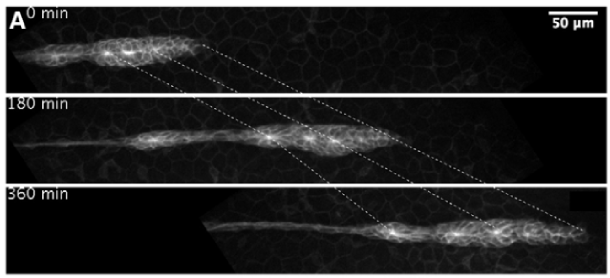
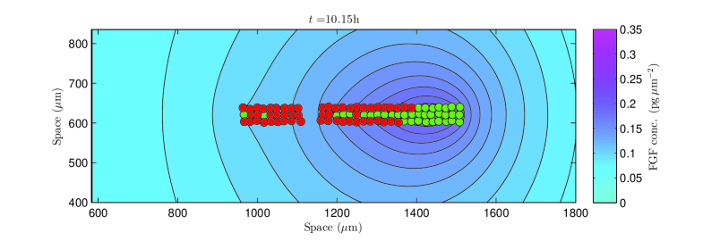
Loosely speaking, lateral line formation consists in a group of mesenchymal cells that migrate driven by a haptotactic signal. In a second phase, a process of differentiation in the rear of the migrating group induces a mesenchymal-epithelial transition that is at the origin of the detachment of rosette-shaped structures. This corresponds to the growth and location of the neuromasts along the two flanks of the primordium (see Figure 1.1 (a) below, from [24]).
Refer to caption
Refer to caption
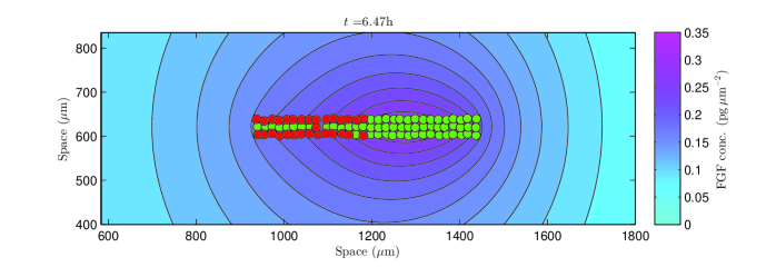
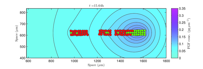
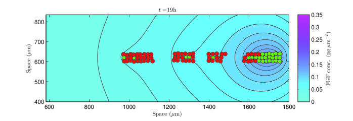
Figure 1.1. (a) Images from a time-lapse movie about the migration in the zebrafish PLL primordium. Leading zone is on the right of the primordium, trailing zone is on the left. Cell migration is to the right while neuromasts deposition occurs in the trailing region (source reproduced with permission from [24]). (b) An example of dynamical simulation of the our mathematical model (see Section 5 for further details).

Our aim is to obtain a minimal mathematical model which is able to:

  1. a)

    describe the collective cell migration, the formation and the detachment of the neuromasts, in the spatial and temporal scale of the experimental observations;

  2. b)

    ensure the existence and stability of the rosette structures of the emerging neuromasts, as stationary solutions of the system.

Request b), among other, allow us to obtain some important restrictions on the range of the values of some parameters of the model, which will be used in the numerical simulations of the dynamical case, other parameters being obtained from biological literature or by a numerical fitting.

The model proposed here is a hybrid model: it describes cells as discrete entities and chemotactic molecules as continuous concentrations. This is a reasonable choice if we think that the total number of cells involved in the morphogenesis process is in the range 80–100 [16, 37]. For analytical and computational simplicity in our analysis, here we consider only the 2D case, although we do not expect great changes passing to 3D, since experimental observations suggest that these phenomena involve only a thin cell layer. As we will see in more detail through numerical simulations given in Section 5, we can state that our mathematical model shows a substantial agreement with the biological observations and with the experimental data proposed in literature (Figure 1.1 (b), to be compared with (a)).

From a mathematical point of view, our model is based on a second order equation of the form

𝐗¨i=𝐅(t,𝐗,𝐗˙,u,u)μ𝐗˙i,subscript¨𝐗𝑖𝐅𝑡𝐗˙𝐗𝑢𝑢𝜇subscript˙𝐗𝑖\displaystyle\ddot{\mathbf{X}}_{i}=\mathbf{F}(t,\mathbf{X},\dot{\mathbf{X}},u,\nabla u)-\mu\dot{\mathbf{X}}_{i},

where 𝐗isubscript𝐗𝑖\mathbf{X}_{i}, i=1,,Ntot𝑖1subscript𝑁toti=1,\dots,N_{\text{tot}}, is the position vector of the i𝑖i-th cell, Ntotsubscript𝑁totN_{\text{tot}} is the total number of cells, 𝐗:=(𝐗1,,𝐗Ntot)assign𝐗subscript𝐗1subscript𝐗subscript𝑁tot\mathbf{X}:=(\mathbf{X}_{1},\dots,\mathbf{X}_{N_{\text{tot}}}), and 𝐗˙:=(𝐗˙1,,𝐗˙Ntot)assign˙𝐗subscript˙𝐗1subscript˙𝐗subscript𝑁tot\dot{\mathbf{X}}:=(\dot{\mathbf{X}}_{1},\dots,\dot{\mathbf{X}}_{N_{\text{tot}}}). The function 𝐅𝐅\mathbf{F} includes several effects: from the detection of chemical signals u𝑢u (chemotaxis, lateral inhibition) to mutual interactions between cells (alignment, adhesion, repulsion). All these effects take into account a non local sensing radius. In particular, we included an alignment term inspired by the Cucker-Smale mechanism [9], though in our case it is coupled with other effects. The term μ𝐗˙i𝜇subscript˙𝐗𝑖-\mu\dot{\mathbf{X}}_{i} represents damping due to cell adhesion to the substrate. Chemical signals are described using a reaction-diffusion equation

tu=DΔu+S(t,𝐗,u),subscript𝑡𝑢𝐷Δ𝑢𝑆𝑡𝐗𝑢\displaystyle\partial_{t}u=D\Delta u+S(t,\mathbf{X},u),

with a possible source or degradation term given in S𝑆S. Finally the cell mesenchymal-epithelial differentiation in the primordium is performed by a switch variable, whose evolution in time is given by a suitable threshold function.

We will show that our model admits particular stationary solutions, biologically relevant and consistent with experimental observations. They correspond to the so called rosettes, that will form the future neuromasts. We investigate numerically their stability, finding in turn a nice agreement with biological evidences both in the stationary and in the dynamical setting.

The paper is organized as follows: in Section 2 we recall some biological backgrounds and the phenomenology, based on the existing experimental observations. In Section 3 the mathematical model is introduced and its main features are discussed. In Section 4 we study the stationary configuration of the rosettes, and their stability. Section 5 deals with the dynamic model. We explain the methods used in the numerical simulations and some 2D numerical tests are presented, with the aim of illustrating the power and the limits of our approach. Section 6 is devoted to the conclusions. Finally, Appendix A contains the lists of main dimensional and nondimensional parameters used in the model.

2. Biological backgrounds

About zebrafish PLL, recent studies and experimental observations [16, 24, 33] show an initial elongated single group of cells in the otic vesicle, in which we can distinguish a trailing region near the head and a leading region oriented towards the future tail of the embryo. In the following few hours after the fertilization, a total cell migration begins posteriorly, from head to tail. Then the cells in the trailing region assemble into rosette structures (proto-neuromast), that are progressively deposed during the migration to form neuromasts [33] (see again Figure 1.1 (a)).

In general we can state two primary mechanisms that concur to this morphogenesis process: a collective migration, and the neuromasts assembly. About cell migration a very important role is played by chemokines as the stromal cell-derived factor-1a (SDF-1a) and its CXCR4b receptor [15, 16]. The former is expressed by the horizontal myoseptum, that separates the dorsal and ventral axial muscles, and acts as a haptotactic stripe for the migrating cells; the latter is expressed by the primordium itself [26]. Chemokine signaling is necessary to drive migration. In fact, it has been proved that, in absence of CXCR4b, cell movements are strongly uncoordinated, with a “zig zag” pattern, as can be seen performing kymograph analysis (see [16]). Moreover, next to the chemoattractant chemokine, migration within the primordium is guaranteed by a cell-cell interaction, exerted by an adhesion force via filopodia. This is confirmed by two observations in [16]: first, cells lacking CXCR4b receptor, transplanted into wild-type primordium, preserve their migration through the contact with neighboring cells; secondly, even a small number of wild-type cells, transplanted in a mutant primordium (lacking the SDF-1a receptor), after moving themselves toward the leading edge can restore the collective migration. In this contest other studies [28, 22, 34, 27, 30] have shown that intercellular adhesion, typically through molecules as the cadherins, and cell-substratum adhesion, through integrins, have a crucial role in the spatial organization of tissues and in embryonic development. Integrin- and cadherin-mediated adhesion allows cells and tissues to respond to mechanical stimuli from their environment and to change shape without loosing integrity ([34] and references therein).

To understand the mechanism which drives the rosettes organization and neuromast deposition (a mechanism however not yet completely described [24]), we have to make some considerations. Neuromast formation is strongly influences by the concentration of fibroblast growth factors (FGFs) and their receptors FGFRs [33, 24]. In zebrafishes, FGF signaling drives cells to assemble rosettes and gives rise to the subdivision of the lateral line. Among the 22 members of the FGF family, only FGF3 and FGF10 are expressed by the primordium [5], and they are substantially equivalent. In fact, inactivation of FGF3 or FGF10 alone does not alter significantly the development of the primordium, demonstrating a robustness of the system [24]. On the other hand, using a FGFR inhibitor SU5402, strongly affects the primordium: cells became disorganized and neuromast deposition stops. In this case also the collective migration is compromised, probably due to an alteration also in CXCR4b receptors [33]. Therefore, the rosette formation depends mainly on the total level of FGF and, as we will see below, on its location. We observe also that FGF and FGFR expressions are mutually exclusive, as confirmed by the location of their molecules: the former, broadly expressed in the leading region, and focused in one or two cells at the center of the rosettes in the trailing region, the latter, at the same time, expressed in the trailing region except the FGF foci [33, 24]. In the aim of designing a mathematical model, this suggests to divide the cell population into two groups: the leader mesenchymal cells (expressing FGF), and the follower epithelial cells (expressing FGFR). At the beginning, all the cells belong to the leading group. Afterwards, few minutes after fertilization, some leaders in the trailing zone start to become followers, except one or two leader cells located in the center, that maintain their mesenchymal state. Loss of FGF activity, on the contrary, implies that no transition can occurs [24]. Then, the follower cells are driven towards the FGF source to form a rosette. As a proto-neuromast becomes fully mature, it is deposited from the trailing edge, and a new rosette is formed again in a cyclic mechanism.

Let us now propose some rules that model the transition from a leader cell into a follower, corresponding to the activation of the FGFR receptor. We assume in the following that the transition occurs under three concomitant conditions:

  1. (1)

    a low level of SDF-1a [15];

  2. (2)

    a high level of FGF [24];

  3. (3)

    a low number of followers in the neighborhood.

The first condition implies that rosette formation begins in the trailing region, where SDF-1a signal is already degraded by cells in the leading edge. The third condition translates a common phenomenon in embryology, the so called lateral inhibition: a cell that adopts a particular feature inhibits its immediate neighbours from doing likewise. This condition, together with the second, implies that followers, activating FGFR receptor, inhibit the same activation in a more surrounded central leader, so that it will express a significantly higher level of FGF signal [18, 21, 19, 29, 31, 39]. Finally we remark that the leader-follower transition can be reversible, possibly with a time delay. In fact, blocking FGF activity makes all cells equally leader and causes the consequent melting of formed rosettes [24].

In the following we will see that our mathematical model will be consistent with the biological observations if we consider chemical effects concomitant with other cell mechanisms, as lateral inhibition, alignment, and adhesion-repulsion effects.

3. The mathematical model

According to the above observations we propose a hybrid model which takes into account the difference between the cellular and the chemical scale. At the cellular level the model is discrete and includes the equation of the motion and the equation of state leader-follower for each single cell, while at the molecular level the model is continuous and is based on the equations for the various chemical signals involved. Let us summarize the main ingredients which compose our model.

For the cell motion we use a second order dynamic equation, which takes into account the forces acting on the cells. These forces are given by chemical signals and mechanical interaction between cells. Because of the equivalence between FGF3 and FGF10, we consider a single concentration and a single receptor, that we will denote respectively as FGF and FGFR. The SDF-1a effect is described by a haptotactic term produced by the gradient of the concentration of this chemokine, see [12] for some biological backgrounds, while mathematical references can be found in [32, 35]. In the same way, the action of FGFR on a follower cell is described by a chemotactic effect due to the gradient of the FGF produced by a leader cell.

Next we describe the cell-cell mechanical interactions due to filopodia, which consist in an alignment effect and both a radial attraction and repulsion depending on the relative position of the cells, see [30] for experimental results in this direction. About alignment effects, we base our description on the seminal paper by F. Cucker and S. Smale [9], while for the attraction-repulsion effects we refer to the mechanism introduced by D’Orsogna et al. [10]; both effects are considered by [1]. Finally, we introduce a damping term, proportional to the velocities, which models cell adhesion to the substrate [36, 14, 2].

The follower-leader differentiation is represented mathematically by a switch state variable, which change its value according to the level of some related functions, which take into account the concentration of SDF-1a and of FGF and also the number of cells in a given neighborhood of the given cell.

About the concentration of the FGF signal we associate a diffusion equation including a source term, given by the FGF production of the leader cells, and a natural molecular degradation term. The concentration of SDF-1a is described by an equation involving its degradation during the haptotactic process.

3.1. The basic mathematical model

Starting from the above considerations, we start to work in the following framework:

acceleration ofi-th cellacceleration ofi-th cell\displaystyle\begin{array}[]{l}\text{acceleration of}\\ \text{$i$-th cell}\end{array} =haptotactic effect of SDF-1aabsenthaptotactic effect of SDF-1a\displaystyle=\text{haptotactic effect of SDF-1a} +chemotactic effect of FGF source on the followerschemotactic effect of FGF source on the followers\displaystyle+\text{chemotactic effect of FGF source on the followers} +cells alignment+cell adhesion and repulsion+damping effectcells alignmentcell adhesion and repulsiondamping effect\displaystyle+\text{cells alignment}+\text{cell adhesion and repulsion}+\text{damping effect} i𝑖i-th cell kind ={followeriflow level of SDF-1a+hight level of FGF+absence of lateral inhibitionleaderotherwiseabsentcasesfolloweriflow level of SDF-1ahight level of FGFmissing-subexpressionmissing-subexpressionabsence of lateral inhibitionleadermissing-subexpressionotherwise\displaystyle=\left\{\begin{array}[]{lll}\text{follower}&\text{if}&\text{low level of SDF-1a}+\text{hight level of FGF}\\ &&+\text{absence of lateral inhibition}\\ \text{leader}&&\text{otherwise}\end{array}\right. rate of change ofFGF signalrate of change ofFGF signal\displaystyle\begin{array}[]{l}\text{rate of change of}\\ \text{FGF signal}\end{array} =diffusion+production+molecular degradationabsentdiffusionproductionmolecular degradation\displaystyle=\text{diffusion}+\text{production}+\text{molecular degradation} rate of change ofSDF-1a signalrate of change ofSDF-1a signal\displaystyle\begin{array}[]{l}\text{rate of change of}\\ \text{SDF-1a signal}\end{array} =degradationabsentdegradation\displaystyle=\text{degradation}

Let 𝐗i(t)subscript𝐗𝑖𝑡\mathbf{X}_{i}(t) be the position of a single i𝑖i-th cell, s(𝐱,t)𝑠𝐱𝑡s(\mathbf{x},t) the SDF-1a concentration, f(𝐱,t)𝑓𝐱𝑡f(\mathbf{x},t) the total FGF concentration (including both FGF3 and FGF10), φi(t)subscript𝜑𝑖𝑡\varphi_{i}(t) a variable that distinguishes a i𝑖i-th cell to be, at time t𝑡t, a leader (φi(t)=1subscript𝜑𝑖𝑡1\varphi_{i}(t)=1) or a follower (φi(t)=0subscript𝜑𝑖𝑡0\varphi_{i}(t)=0). We introduce the following equations:

{𝐗¨i=α𝐅1(s)+γ(1φi)𝐅1(f)+𝐅2(𝐗˙)+𝐅3(𝐗)[μF+(μLμF)φi]𝐗˙i,φi={0,ifδF1(s)[kF+(kLkF)φi]F1(h(f))+λΓ(ni)0,1,otherwise,tf=DΔf+ξF4(𝐗)ηf,ts=σsF5(𝐗),casessubscript¨𝐗𝑖absent𝛼subscript𝐅1𝑠𝛾1subscript𝜑𝑖subscript𝐅1𝑓subscript𝐅2˙𝐗subscript𝐅3𝐗delimited-[]subscript𝜇Fsubscript𝜇Lsubscript𝜇Fsubscript𝜑𝑖subscript˙𝐗𝑖missing-subexpressionmissing-subexpressionsubscript𝜑𝑖absentcases0if𝛿subscript𝐹1𝑠delimited-[]subscript𝑘Fsubscript𝑘Lsubscript𝑘Fsubscript𝜑𝑖subscript𝐹1𝑓𝜆Γsubscript𝑛𝑖01missing-subexpressionotherwisemissing-subexpressionmissing-subexpressionsubscript𝑡𝑓absent𝐷Δ𝑓𝜉subscript𝐹4𝐗𝜂𝑓missing-subexpressionmissing-subexpressionsubscript𝑡𝑠absent𝜎𝑠subscript𝐹5𝐗\left\{\begin{array}[]{rl}\ddot{\mathbf{X}}_{i}&=\alpha\mathbf{F}_{1}\left(\nabla s\right)+\gamma(1-\varphi_{i})\mathbf{F}_{1}\left(\nabla f\right)+\mathbf{F}_{2}(\dot{\mathbf{X}})+\mathbf{F}_{3}(\mathbf{X})-\left[\mu_{\text{F}}+(\mu_{\text{L}}-\mu_{\text{F}})\varphi_{i}\right]\dot{\mathbf{X}}_{i},\\ \\ \varphi_{i}&=\left\{\begin{array}[]{lll}0,&\text{if}&\delta F_{1}(s)-\left[k_{\text{F}}+(k_{\text{L}}-k_{\text{F}})\varphi_{i}\right]F_{1}(h(f))+\lambda\Gamma(n_{i})\leq 0,\\ 1,&&\text{otherwise},\end{array}\right.\\ \\ \partial_{t}f&=D\Delta f+\xi F_{4}(\mathbf{X})-\eta f,\\ \\ \partial_{t}s&=-\sigma sF_{5}(\mathbf{X}),\end{array}\right. (3.1)

where α𝛼\alpha, γ𝛾\gamma, μLsubscript𝜇L\mu_{\text{L}}, μFsubscript𝜇F\mu_{\text{F}}, δ𝛿\delta, kLsubscript𝑘Lk_{\text{L}}, kFsubscript𝑘Fk_{\text{F}}, λ𝜆\lambda, D𝐷D, ξ𝜉\xi, η𝜂\eta, σ𝜎\sigma are given positive constants, and Fn()subscript𝐹𝑛F_{n}(\cdot), n=1,,5𝑛15n=1,\dots,5, are suitable functions.

The term F1subscript𝐹1F_{1}, which is related to the detection of a chemical signal by i𝑖i-th cell in its neighborhood, is taken to be a weighted average over a ball of radius R¯¯𝑅\bar{R} and centered in 𝐗isubscript𝐗𝑖\mathbf{X}_{i}:

F1(g(𝐱,t)):=1W𝐁(𝐗i,R¯)g(𝐱,t)wi(𝐱)𝑑𝐱,assignsubscript𝐹1𝑔𝐱𝑡1𝑊subscript𝐁subscript𝐗𝑖¯𝑅𝑔𝐱𝑡subscript𝑤𝑖𝐱differential-d𝐱\displaystyle F_{1}(g(\mathbf{x},t)):=\frac{1}{W}\int_{\mathbf{B}(\mathbf{X}_{i},\bar{R})}g(\mathbf{x},t)w_{i}(\mathbf{x})\,d\mathbf{x}, (3.2)

where

𝐁(𝐗i,R¯):={𝐱:𝐱𝐗iR¯},assign𝐁subscript𝐗𝑖¯𝑅conditional-set𝐱norm𝐱subscript𝐗𝑖¯𝑅\displaystyle\mathbf{B}(\mathbf{X}_{i},\bar{R}):=\left\{\mathbf{x}:\left|\left|\mathbf{x}-\mathbf{X}_{i}\right|\right|\leq\bar{R}\right\}, (3.3)

||||\left|\left|\cdot\right|\right| being the Euclidean norm,

wi(𝐱):={2exp(𝐱𝐗i2log2R¯2)1,if𝐱𝐗iR¯;0,otherwise;assignsubscript𝑤𝑖𝐱cases2superscriptnorm𝐱subscript𝐗𝑖22superscript¯𝑅21ifnorm𝐱subscript𝐗𝑖¯𝑅0missing-subexpressionotherwise\displaystyle w_{i}(\mathbf{x}):=\left\{\begin{array}[]{lll}2\exp\left(-||\mathbf{x}-\mathbf{X}_{i}||^{2}\displaystyle\frac{\log 2}{\bar{R}^{2}}\right)-1,&\text{if}&||\mathbf{x}-\mathbf{X}_{i}||\leq\bar{R};\\ 0,&&\text{otherwise};\end{array}\right. (3.6)

is a truncated Gaussian weight function, and

W:=𝐁(𝐗i,R¯)wi(𝐱)𝑑𝐱,assign𝑊subscript𝐁subscript𝐗𝑖¯𝑅subscript𝑤𝑖𝐱differential-d𝐱\displaystyle W:=\int_{\mathbf{B}(\mathbf{X}_{i},\bar{R})}w_{i}(\mathbf{x})\,d\mathbf{x}, (3.7)

independently of i𝑖i. A similar definition holds for the vector quantity 𝐅1subscript𝐅1\mathbf{F}_{1}. Reasonably we will choose R¯¯𝑅\bar{R} larger than the cell radius R𝑅R (see Appendix A), so (3.2) describes a chemical signal that is sensed more in the center of the cell and less at the edge of the cell extensions. The second addend in (3.1)1 refers to the attraction of a follower cell toward a source of FGF ligand. The switch variable φisubscript𝜑𝑖\varphi_{i} makes this term zero for a leader cell that, expressing FGF, does not activate FGFR receptor (see Section 2).

The effect included in the third addend of (3.1)1 represents a possible cell alignment. For it we assume a Cucker-Smale flocking term:

𝐅2(𝐗˙):=1N¯ij:𝐗j𝐁(𝐗i,R1)\{𝐗i}𝐇(𝐗˙j𝐗˙i).assignsubscript𝐅2˙𝐗1subscript¯𝑁𝑖subscript:𝑗subscript𝐗𝑗\𝐁subscript𝐗𝑖subscript𝑅1subscript𝐗𝑖𝐇subscript˙𝐗𝑗subscript˙𝐗𝑖\displaystyle\mathbf{F}_{2}(\dot{\mathbf{X}}):=\frac{1}{\bar{N}_{i}}\sum_{j:\mathbf{X}_{j}\in\mathbf{B}(\mathbf{X}_{i},R_{1})\backslash\left\{\mathbf{X}_{i}\right\}}\mathbf{H}(\dot{\mathbf{X}}_{j}-\dot{\mathbf{X}}_{i}). (3.8)

Here R1subscript𝑅1R_{1} is a suitable radius of influence,

N¯i:=card{j:𝐗j𝐁(𝐗i,R1)\{𝐗i}},assignsubscript¯𝑁𝑖cardconditional-set𝑗subscript𝐗𝑗\𝐁subscript𝐗𝑖subscript𝑅1subscript𝐗𝑖\displaystyle\bar{N}_{i}:=\text{card}\left\{j:\mathbf{X}_{j}\in\mathbf{B}(\mathbf{X}_{i},R_{1})\backslash\left\{\mathbf{X}_{i}\right\}\right\}, (3.9)

and the function 𝐇𝐇\mathbf{H} depends on the relative velocities 𝐗˙j𝐗˙isubscript˙𝐗𝑗subscript˙𝐗𝑖\dot{\mathbf{X}}_{j}-\dot{\mathbf{X}}_{i}, i.e.:

𝐇(𝐗˙j𝐗˙i):=[βF+(βLβF)φiφj]R12R12+𝐗j𝐗i2(𝐗˙j𝐗˙i),assign𝐇subscript˙𝐗𝑗subscript˙𝐗𝑖delimited-[]subscript𝛽Fsubscript𝛽Lsubscript𝛽Fsubscript𝜑𝑖subscript𝜑𝑗superscriptsubscript𝑅12superscriptsubscript𝑅12superscriptnormsubscript𝐗𝑗subscript𝐗𝑖2subscript˙𝐗𝑗subscript˙𝐗𝑖\displaystyle\mathbf{H}(\dot{\mathbf{X}}_{j}-\dot{\mathbf{X}}_{i}):=\left[\beta_{\text{F}}+(\beta_{\text{L}}-\beta_{\text{F}})\varphi_{i}\varphi_{j}\right]\frac{R_{1}^{2}}{R_{1}^{2}+||\mathbf{X}_{j}-\mathbf{X}_{i}||^{2}}(\dot{\mathbf{X}}_{j}-\dot{\mathbf{X}}_{i}), (3.10)

βFsubscript𝛽F\beta_{\text{F}}, βLsubscript𝛽L\beta_{\text{L}} being constants. In particular we can have different coefficient of alignment for a leader or follower cell: the product φiφjsubscript𝜑𝑖subscript𝜑𝑗\varphi_{i}\varphi_{j} makes the coefficient equal to βFsubscript𝛽F\beta_{\text{F}} if at least one of the two cell is follower (φiφj=0subscript𝜑𝑖subscript𝜑𝑗0\varphi_{i}\varphi_{j}=0) and equal to βLsubscript𝛽L\beta_{\text{L}} in the case of two leaders (φiφj=1subscript𝜑𝑖subscript𝜑𝑗1\varphi_{i}\varphi_{j}=1). We remark that the flocking term given by (3.10), which is studied in [9, 17], in our model is coupled with other effects, as chemotaxis and attraction-repulsion effects (see below), and it is also computed on a truncated domain. In the following we will assume R1=R¯subscript𝑅1¯𝑅R_{1}=\bar{R} (see Appendix A), but in principle they can be different.

Function 𝐅3subscript𝐅3\mathbf{F}_{3} includes adhesion-repulsion effects. In particular repulsion occurs at a distance between the centers of two cells less than R4subscript𝑅4R_{4} and takes into account the effects of a possible cell deformation. Conversely, adhesion occurs at a distance greater than R4subscript𝑅4R_{4} and less than R5>R4subscript𝑅5subscript𝑅4R_{5}>R_{4}, and it is due to a mechanical interaction between cells via filopodia. We assume

𝐅3(𝐗):=j:𝐗j𝐁(𝐗i,R5)\{𝐗i}𝐊(𝐗j𝐗i),assignsubscript𝐅3𝐗subscript:𝑗subscript𝐗𝑗\𝐁subscript𝐗𝑖subscript𝑅5subscript𝐗𝑖𝐊subscript𝐗𝑗subscript𝐗𝑖\displaystyle\mathbf{F}_{3}(\mathbf{X}):=\sum_{j:\mathbf{X}_{j}\in\mathbf{B}(\mathbf{X}_{i},R_{5})\backslash\left\{\mathbf{X}_{i}\right\}}\mathbf{K}(\mathbf{X}_{j}-\mathbf{X}_{i}), (3.11)

where the function 𝐊𝐊\mathbf{K} depends on the relative positions 𝐗j𝐗isubscript𝐗𝑗subscript𝐗𝑖\mathbf{X}_{j}-\mathbf{X}_{i}, i.e.:

𝐊(𝐗j𝐗i):={ωrep(1𝐗j𝐗i1R4)𝐗j𝐗i𝐗j𝐗i,if𝐗j𝐗iR4;[ωadh,F+(ωadh,Lωadh,F)φiφj](𝐗j𝐗iR4)𝐗j𝐗i𝐗j𝐗i,ifR4<𝐗j𝐗iR5;assign𝐊subscript𝐗𝑗subscript𝐗𝑖casessubscript𝜔rep1normsubscript𝐗𝑗subscript𝐗𝑖1subscript𝑅4subscript𝐗𝑗subscript𝐗𝑖normsubscript𝐗𝑗subscript𝐗𝑖ifnormsubscript𝐗𝑗subscript𝐗𝑖subscript𝑅4missing-subexpressionmissing-subexpressionmissing-subexpressiondelimited-[]subscript𝜔adh,Fsubscript𝜔adh,Lsubscript𝜔adh,Fsubscript𝜑𝑖subscript𝜑𝑗normsubscript𝐗𝑗subscript𝐗𝑖subscript𝑅4subscript𝐗𝑗subscript𝐗𝑖normsubscript𝐗𝑗subscript𝐗𝑖ifsubscript𝑅4normsubscript𝐗𝑗subscript𝐗𝑖subscript𝑅5\displaystyle\mathbf{K}(\mathbf{X}_{j}-\mathbf{X}_{i}):=\left\{\begin{array}[]{lll}-\omega_{\text{rep}}\left(\displaystyle\frac{1}{||\mathbf{X}_{j}-\mathbf{X}_{i}||}-\frac{1}{R_{4}}\right)\displaystyle\frac{\mathbf{X}_{j}-\mathbf{X}_{i}}{||\mathbf{X}_{j}-\mathbf{X}_{i}||},&\text{if}&||\mathbf{X}_{j}-\mathbf{X}_{i}||\leq R_{4};\\ \\ \left[\omega_{\text{adh,F}}+(\omega_{\text{adh,L}}-\omega_{\text{adh,F}})\varphi_{i}\varphi_{j}\right]\left(||\mathbf{X}_{j}-\mathbf{X}_{i}||-R_{4}\right)\displaystyle\frac{\mathbf{X}_{j}-\mathbf{X}_{i}}{||\mathbf{X}_{j}-\mathbf{X}_{i}||},&\text{if}&R_{4}<||\mathbf{X}_{j}-\mathbf{X}_{i}||\leq R_{5};\end{array}\right. (3.15)

ωrepsubscript𝜔rep\omega_{\text{rep}}, ωadh,Lsubscript𝜔adh,L\omega_{\text{adh,L}}, ωadh,Fsubscript𝜔adh,F\omega_{\text{adh,F}} being constants. In practice we will choose R4=2Rsubscript𝑅42𝑅R_{4}=2R (see Appendix A), so that repulsion occurs when two cells start to be effectively overlapped. We note that function (3.15)1 gives a repulsion which goes as 1/r1𝑟1/r, r𝑟r being the distance between the centers of two cells, as we can find in [8, 38]. The function (3.15)2 represents Hooke’s law of elasticity, with different elastic coefficients for a leader cell and for a follower. In particular we have ωadh,Fsubscript𝜔adh,F\omega_{\text{adh,F}} if at least one of the two cells is a follower (φiφj=0subscript𝜑𝑖subscript𝜑𝑗0\varphi_{i}\varphi_{j}=0) and ωadh,L>ωadh,Fsubscript𝜔adh,Lsubscript𝜔adh,F\omega_{\text{adh,L}}>\omega_{\text{adh,F}} if two cells are both leader (φiφj=1subscript𝜑𝑖subscript𝜑𝑗1\varphi_{i}\varphi_{j}=1). Similar terms can be found in [1] and references therein. We remark that adhesion (3.15)2 and alignment (3.10) produce different effects, though they both refer to a cell-cell interaction: the former a radial effect, the latter a tangential effect.

The last term in the first equation is due to the cell adhesion to the substrate (see for example [36, 14, 2]), possibly with a different damping coefficient for a leader (μLsubscript𝜇L\mu_{\text{L}}, given by φi=1subscript𝜑𝑖1\varphi_{i}=1) or a follower cell (μFsubscript𝜇F\mu_{\text{F}}, given by φi=0subscript𝜑𝑖0\varphi_{i}=0).

The second equation in (3.1) defines the switch variable φisubscript𝜑𝑖\varphi_{i} for the i𝑖i-th cell. The leader-to-follower transition is performed requiring that the threshold function at the right hand side of (3.1)2 is less than zero, according with the three conditions described in Section 2. For the FGF detection in F1(h(f))subscript𝐹1𝑓F_{1}(h(f)) we choose the following form for the function h(f)𝑓h(f):

h(f):=ffmax+f,assign𝑓𝑓subscript𝑓𝑓\displaystyle h(f):=\frac{f}{f_{\max}+f}, (3.16)

where fmaxsubscript𝑓f_{\max} is constant. The function (3.16) includes a possible saturation effect when FGF molecules tend to occupy all receptors of a cell. The coefficients kLsubscript𝑘Lk_{\text{L}} and kFsubscript𝑘Fk_{\text{F}}, related respectively to a leader and a follower cell, provides a delay in the inverse follower-to-leader transition setting suitably kL<kFsubscript𝑘Lsubscript𝑘Fk_{\text{L}}<k_{\text{F}}, this in accordance to observations in Section 2. About the lateral inhibition mechanism, we introduce a function Γ(ni)Γsubscript𝑛𝑖\Gamma(n_{i}) that counts the number nisubscript𝑛𝑖n_{i} of cells in a suitable neighborhood of the i𝑖i-th cell, with radius of influence R2subscript𝑅2R_{2}, namely

Γ(ni):=enieni+Γ011+Γ0,assignΓsubscript𝑛𝑖superscript𝑒subscript𝑛𝑖superscript𝑒subscript𝑛𝑖subscriptΓ011subscriptΓ0\displaystyle\Gamma(n_{i}):=\frac{e^{n_{i}}}{e^{n_{i}}+\Gamma_{0}}-\frac{1}{1+\Gamma_{0}}, (3.17)

where

ni:=card{j:𝐗j𝐁̊(𝐗i,R2)\{𝐗i}},assignsubscript𝑛𝑖cardconditional-set𝑗subscript𝐗𝑗\̊𝐁subscript𝐗𝑖subscript𝑅2subscript𝐗𝑖\displaystyle n_{i}:=\text{card}\left\{j:\mathbf{X}_{j}\in\mathring{\mathbf{B}}(\mathbf{X}_{i},R_{2})\backslash\left\{\mathbf{X}_{i}\right\}\right\}, (3.18)

Γ0subscriptΓ0\Gamma_{0} is a constant, and 𝐁̊(𝐗i,R2)̊𝐁subscript𝐗𝑖subscript𝑅2\mathring{\mathbf{B}}(\mathbf{X}_{i},R_{2}) is the interior of 𝐁(𝐗i,R2)𝐁subscript𝐗𝑖subscript𝑅2\mathbf{B}(\mathbf{X}_{i},R_{2}). Function (3.17) is justified if we think of a neuromast as made by a single central leader and some followers around. In this contest it makes an appropriate difference between the number of cells counted by the central cell and those counted by a lateral cell. Moreover, it provides a fast saturation effect when n𝑛n increases, so that a central leader counts about the same number of cells from a certain value of n𝑛n. This is useful to describe the possibility to obtain neuromasts with a variable number of cells, according to experimental observations (generally 8-20 cells) [24]. A suitable value for the constant Γ0subscriptΓ0\Gamma_{0} is given in Appendix A.

In the diffusion equation (3.1)3, only leader cells are responsible of the production of FGF, so that

F4(𝐗):=j=1Ntotφjχ𝐁(𝐗j,R3),assignsubscript𝐹4𝐗superscriptsubscript𝑗1subscript𝑁totsubscript𝜑𝑗subscript𝜒𝐁subscript𝐗𝑗subscript𝑅3\displaystyle F_{4}(\mathbf{X}):=\sum_{j=1}^{N_{\text{tot}}}\varphi_{j}\chi_{\mathbf{B}(\mathbf{X}_{j},R_{3})}, (3.19)

where Ntotsubscript𝑁totN_{\text{tot}} is the total number of cells, and

χ𝐁(𝐗j,R3):={1,if𝐱𝐁(𝐗j,R3);0,otherwise.assignsubscript𝜒𝐁subscript𝐗𝑗subscript𝑅3cases1if𝐱𝐁subscript𝐗𝑗subscript𝑅30missing-subexpressionotherwise\displaystyle\chi_{\mathbf{B}(\mathbf{X}_{j},R_{3})}:=\left\{\begin{array}[]{lll}1,&\text{if}&\mathbf{x}\in\mathbf{B}(\mathbf{X}_{j},R_{3});\\ 0,&&\text{otherwise}.\end{array}\right. (3.22)

Similarly, in equation (3.1)4 we take

F5(𝐗):=j=1Ntotχ𝐁(𝐗j,R3),assignsubscript𝐹5𝐗superscriptsubscript𝑗1subscript𝑁totsubscript𝜒𝐁subscript𝐗𝑗subscript𝑅3\displaystyle F_{5}(\mathbf{X}):=\sum_{j=1}^{N_{\text{tot}}}\displaystyle\chi_{\mathbf{B}(\mathbf{X}_{j},R_{3})},

in which the variable φ𝜑\varphi does not appear now, because both leaders and followers are involved in the haptotactic process. Typically, we will choose R3=Rsubscript𝑅3𝑅R_{3}=R considering that the source of FGF and the degradation of SDF-1a signal is substantially defined by the dimension of a single cell (see Appendix A).

The above observations let us to summarize the following model:

{𝐗¨i=αW𝐁(𝐗i,R¯)s(𝐱,t)wi(𝐱)𝑑𝐱+γ(1φi)W𝐁(𝐗i,R¯)f(𝐱,t)wi(𝐱)𝑑𝐱+1N¯ij:𝐗j𝐁(𝐗i,R1)\{𝐗i}𝐇(𝐗˙j𝐗˙i)+j:𝐗j𝐁(𝐗i,R5)\{𝐗i}𝐊(𝐗j𝐗i)[μF+(μLμF)φi]𝐗˙i,φi={0ifδW𝐁(𝐗i,R¯)s(𝐱,t)wi(𝐱)𝑑𝐱kF+(kLkF)φiW𝐁(𝐗i,R¯)f(𝐱,t)fmax+f(𝐱,t)wi(𝐱)𝑑𝐱+λΓ(ni)0,1otherwise,tf=DΔf+ξj=1Ntotφjχ𝐁(𝐗j,R3)ηf,ts=σsj=1Ntotχ𝐁(𝐗j,R3),casessubscript¨𝐗𝑖absent𝛼𝑊subscript𝐁subscript𝐗𝑖¯𝑅𝑠𝐱𝑡subscript𝑤𝑖𝐱differential-d𝐱𝛾1subscript𝜑𝑖𝑊subscript𝐁subscript𝐗𝑖¯𝑅𝑓𝐱𝑡subscript𝑤𝑖𝐱differential-d𝐱missing-subexpressionmissing-subexpressionmissing-subexpressionmissing-subexpressionmissing-subexpression1subscript¯𝑁𝑖subscript:𝑗subscript𝐗𝑗\𝐁subscript𝐗𝑖subscript𝑅1subscript𝐗𝑖𝐇subscript˙𝐗𝑗subscript˙𝐗𝑖subscript:𝑗subscript𝐗𝑗\𝐁subscript𝐗𝑖subscript𝑅5subscript𝐗𝑖𝐊subscript𝐗𝑗subscript𝐗𝑖delimited-[]subscript𝜇Fsubscript𝜇Lsubscript𝜇Fsubscript𝜑𝑖subscript˙𝐗𝑖missing-subexpressionmissing-subexpressionmissing-subexpressionmissing-subexpressionsubscript𝜑𝑖absentcases0if𝛿𝑊subscript𝐁subscript𝐗𝑖¯𝑅𝑠𝐱𝑡subscript𝑤𝑖𝐱differential-d𝐱subscript𝑘Fsubscript𝑘Lsubscript𝑘Fsubscript𝜑𝑖𝑊subscript𝐁subscript𝐗𝑖¯𝑅𝑓𝐱𝑡subscript𝑓max𝑓𝐱𝑡subscript𝑤𝑖𝐱differential-d𝐱missing-subexpressionmissing-subexpressionmissing-subexpressionmissing-subexpressionmissing-subexpression𝜆Γsubscript𝑛𝑖0missing-subexpressionmissing-subexpressionmissing-subexpression1missing-subexpressionotherwisemissing-subexpressionmissing-subexpressionmissing-subexpressionmissing-subexpressionsubscript𝑡𝑓absent𝐷Δ𝑓𝜉superscriptsubscript𝑗1subscript𝑁totsubscript𝜑𝑗subscript𝜒𝐁subscript𝐗𝑗subscript𝑅3𝜂𝑓missing-subexpressionmissing-subexpressionmissing-subexpressionmissing-subexpressionsubscript𝑡𝑠absent𝜎𝑠superscriptsubscript𝑗1subscript𝑁totsubscript𝜒𝐁subscript𝐗𝑗subscript𝑅3missing-subexpression\begin{split}&\left\{\begin{array}[]{lll}\ddot{\mathbf{X}}_{i}&=\displaystyle\frac{\alpha}{W}\int_{\mathbf{B}(\mathbf{X}_{i},\bar{R})}\nabla s(\mathbf{x},t)w_{i}(\mathbf{x})\,d\mathbf{x}+\displaystyle\frac{\gamma(1-\varphi_{i})}{W}\int_{\mathbf{B}(\mathbf{X}_{i},\bar{R})}\nabla f(\mathbf{x},t)w_{i}(\mathbf{x})\,d\mathbf{x}\\ \\ &+\displaystyle\frac{1}{\bar{N}_{i}}\sum_{j:\mathbf{X}_{j}\in\mathbf{B}(\mathbf{X}_{i},R_{1})\backslash\left\{\mathbf{X}_{i}\right\}}\mathbf{H}(\dot{\mathbf{X}}_{j}-\dot{\mathbf{X}}_{i})+\sum_{j:\mathbf{X}_{j}\in\mathbf{B}(\mathbf{X}_{i},R_{5})\backslash\left\{\mathbf{X}_{i}\right\}}\mathbf{K}(\mathbf{X}_{j}-\mathbf{X}_{i})-\left[\mu_{\text{F}}+(\mu_{\text{L}}-\mu_{\text{F}})\varphi_{i}\right]\dot{\mathbf{X}}_{i},\\ \\ \displaystyle\varphi_{i}&\displaystyle=\left\{\begin{array}[]{lll}0&\text{if}&\displaystyle\frac{\delta}{W}\int_{\mathbf{B}(\mathbf{X}_{i},\bar{R})}s(\mathbf{x},t)w_{i}(\mathbf{x})\,d\mathbf{x}-\frac{k_{\text{F}}+(k_{\text{L}}-k_{\text{F}})\varphi_{i}}{W}\int_{\mathbf{B}(\mathbf{X}_{i},\bar{R})}\frac{f(\mathbf{x},t)}{f_{\text{max}}+f(\mathbf{x},t)}w_{i}(\mathbf{x})\,d\mathbf{x}\\ \\ &&+\displaystyle\lambda\Gamma(n_{i})\leq 0,\\ \\ 1&&\text{otherwise},\end{array}\right.\\ \\ \displaystyle\partial_{t}f&\displaystyle=D\Delta f+\xi\sum_{j=1}^{N_{\text{tot}}}\displaystyle\varphi_{j}\chi_{\mathbf{B}(\mathbf{X}_{j},R_{3})}-\eta f,\\ \\ \displaystyle\partial_{t}s&\displaystyle=-\sigma s\sum_{j=1}^{N_{\text{tot}}}\displaystyle\chi_{\mathbf{B}(\mathbf{X}_{j},R_{3})},\end{array}\right.\\ \end{split} (3.23)

where the functions 𝐇(𝐗˙j𝐗˙i)𝐇subscript˙𝐗𝑗subscript˙𝐗𝑖\mathbf{H}(\dot{\mathbf{X}}_{j}-\dot{\mathbf{X}}_{i}) and 𝐊(𝐗j𝐗i)𝐊subscript𝐗𝑗subscript𝐗𝑖\mathbf{K}(\mathbf{X}_{j}-\mathbf{X}_{i}) are given by (3.10) and (3.15). Initial and boundary conditions have to be specified. For the i𝑖i-th cell we set

𝐗i(0)=𝐗i0;and𝐗˙i(0)=𝟎,i=1,,Ntot,formulae-sequencesubscript𝐗𝑖0subscript𝐗𝑖0andformulae-sequencesubscript˙𝐗𝑖00𝑖1subscript𝑁tot\displaystyle\mathbf{X}_{i}(0)=\mathbf{X}_{i0};\quad\mbox{and}\quad\dot{\mathbf{X}}_{i}(0)=\mathbf{0},\quad i=1,\dots,N_{\text{tot}}, (3.24)

together with the equally initial cell state of leader:

φi(0)=1,i=1,,Ntot.formulae-sequencesubscript𝜑𝑖01𝑖1subscript𝑁tot\displaystyle\varphi_{i}(0)=1,\quad i=1,\dots,N_{\text{tot}}. (3.25)

Now, let Ω=[a,b]×[c,d]Ω𝑎𝑏𝑐𝑑\Omega=[a,b]\times[c,d] our domain, for FGF signal we require zero initial concentration and homogeneous Neumann boundary condition:

f(𝐱,0)=0;f𝐧=0,on Ω.formulae-sequence𝑓𝐱00𝑓𝐧0on Ω\displaystyle f(\mathbf{x},0)=0;\quad\frac{\partial f}{\partial\mathbf{n}}=0,\quad\mbox{on $\partial\Omega$}. (3.26)

No-flow boundary condition (3.26)2 is justified if we think of an experiment in which our domain is isolated from the surrounding environment. Then, since initially SDF-1a is only located in a given region

s(𝐱,0)=s0(𝐱),𝑠𝐱0subscript𝑠0𝐱\displaystyle s(\mathbf{x},0)=s_{0}(\mathbf{x}), (3.27)

where s0(𝐱)subscript𝑠0𝐱s_{0}(\mathbf{x}) has compact support in ΩΩ\Omega. In particular we consider a rectangular stripe of width 2l2𝑙2l, [a¯,b¯]×[ml,m+l]¯𝑎¯𝑏𝑚𝑙𝑚𝑙[\bar{a},\bar{b}]\times[m-l,m+l], with [a¯,b¯][a,b]¯𝑎¯𝑏𝑎𝑏[\bar{a},\bar{b}]\subset[a,b], m=(c+d)/2𝑚𝑐𝑑2m=(c+d)/2, and

s0(x,y):=Φ(x)Ψ(y),assignsubscript𝑠0𝑥𝑦Φ𝑥Ψ𝑦\displaystyle s_{0}(x,y):=\Phi(x)\Psi(y), (3.28)

where, for instance, we choose

Φ(x):=smax2[tanh(xc1c2)+1]χ[a¯,b¯],assignΦ𝑥subscript𝑠2delimited-[]𝑥subscript𝑐1subscript𝑐21subscript𝜒¯𝑎¯𝑏\displaystyle\Phi(x):=\frac{s_{\max}}{2}\left[\tanh\left(\frac{x-c_{1}}{c_{2}}\right)+1\right]\chi_{[\bar{a},\bar{b}]}, (3.29)

smaxsubscript𝑠s_{\max} is the initial maximum SDF-1a concentration, c1subscript𝑐1c_{1}, c2subscript𝑐2c_{2} are constants. Function (3.29) yields a non uniform haptotactic gradient, that is stronger at the beginning and then tends to saturate when cells acquire enough velocity. Values for c1subscript𝑐1c_{1}, c2subscript𝑐2c_{2} will be given in Section 5. Then we set

Ψ(y):=uε(y)χ[ml,m+l](y)=cduε(yτ)χ[ml,m+l](y)𝑑τ,assignΨ𝑦subscript𝑢𝜀𝑦subscript𝜒𝑚𝑙𝑚𝑙𝑦subscriptsuperscript𝑑𝑐subscript𝑢𝜀𝑦𝜏subscript𝜒𝑚𝑙𝑚𝑙𝑦differential-d𝜏\displaystyle\Psi(y):=u_{\varepsilon}(y)\ast\chi_{[m-l,m+l]}(y)=\int^{d}_{c}u_{\varepsilon}(y-\tau)\chi_{[m-l,m+l]}(y)\,d\tau, (3.30)

the convolution of χ[ml,m+l](y)subscript𝜒𝑚𝑙𝑚𝑙𝑦\chi_{[m-l,m+l]}(y) with a positive and symmetric mollifier

uε(y)subscript𝑢𝜀𝑦\displaystyle u_{\varepsilon}(y) :={1J1εe11(y/ε)2,ifε<y<ε;0,otherwise;assignabsentcases1𝐽1𝜀superscript𝑒11superscript𝑦𝜀2if𝜀𝑦𝜀missing-subexpressionmissing-subexpressionmissing-subexpression0missing-subexpressionotherwise\displaystyle:=\left\{\begin{array}[]{lll}\displaystyle\frac{1}{J}\frac{1}{\varepsilon}\;e^{-\displaystyle\frac{1}{1-\left(y/\varepsilon\right)^{2}}},&\text{if}&-\varepsilon<y<\varepsilon;\\ \\ 0,&&\text{otherwise};\end{array}\right. (3.34)

where

J𝐽\displaystyle J :=εε1εe11(y/ε)2𝑑y,assignabsentsuperscriptsubscript𝜀𝜀1𝜀superscript𝑒11superscript𝑦𝜀2differential-d𝑦\displaystyle:=\int_{-\varepsilon}^{\varepsilon}\frac{1}{\varepsilon}\;e^{-\displaystyle\frac{1}{1-\left(y/\varepsilon\right)^{2}}}\,dy, (3.35)

is the normalization factor. Mollifier (3.34) is introduced to have sufficient smoothness for s0(𝐱)subscript𝑠0𝐱s_{0}(\mathbf{x}). A suitable value for the positive constant ε𝜀\varepsilon will be given in Section 5.

3.2. The nondimensional model

Though we tend to use dimensional times and distances in the plots for easier comparison with experiments, the qualitative behaviour of the model (3.23) is more clearly described using a nondimensional based on the following dimensionless quantities:

t:=tT,𝐱:=𝐱R,𝐗:=𝐗R,f:=ffmax,s:=ssmax,W:=WR2,Ri:=RiRi=1,,5,R¯:=R¯R,α:=αsmaxT2R2,βL:=βLT,βF:=βFT,γ:=γfmaxT2R2,ωrep:=ωrepT2R2,ωadh,L:=ωadh,LT2,ωadh,F:=ωadh,FT2,μL:=μLT,μF:=μFT,δ:=δsmaxλ,kL:=kLλ,kF:=kFλ,D:=DTR2,ξ:=ξTfmax,η:=ηT,σ:=σT,c1:=c1R,c2:=c2R,ε:=εR,formulae-sequenceformulae-sequenceassignsuperscript𝑡𝑡𝑇formulae-sequenceassignsuperscript𝐱𝐱𝑅formulae-sequenceassignsuperscript𝐗𝐗𝑅formulae-sequenceassignsuperscript𝑓𝑓subscript𝑓formulae-sequenceassignsuperscript𝑠𝑠subscript𝑠formulae-sequenceassignsuperscript𝑊𝑊superscript𝑅2assignsuperscriptsubscript𝑅𝑖subscript𝑅𝑖𝑅𝑖1assign5superscript¯𝑅¯𝑅𝑅formulae-sequenceassignsuperscript𝛼𝛼subscript𝑠superscript𝑇2superscript𝑅2formulae-sequenceassignsubscriptsuperscript𝛽Lsubscript𝛽L𝑇formulae-sequenceassignsubscriptsuperscript𝛽Fsubscript𝛽F𝑇formulae-sequenceassignsuperscript𝛾𝛾subscript𝑓superscript𝑇2superscript𝑅2formulae-sequenceassignsubscriptsuperscript𝜔repsubscript𝜔repsuperscript𝑇2superscript𝑅2formulae-sequenceassignsubscriptsuperscript𝜔adh,Lsubscript𝜔adh,Lsuperscript𝑇2formulae-sequenceassignsubscriptsuperscript𝜔adh𝐹subscript𝜔adh,Fsuperscript𝑇2formulae-sequenceassignsubscriptsuperscript𝜇𝐿subscript𝜇L𝑇formulae-sequenceassignsubscriptsuperscript𝜇Fsubscript𝜇F𝑇formulae-sequenceassignsuperscript𝛿𝛿subscript𝑠𝜆formulae-sequenceassignsubscriptsuperscript𝑘Lsubscript𝑘L𝜆formulae-sequenceassignsubscriptsuperscript𝑘Fsubscript𝑘F𝜆formulae-sequenceassignsuperscript𝐷𝐷𝑇superscript𝑅2formulae-sequenceassignsuperscript𝜉𝜉𝑇subscript𝑓formulae-sequenceassignsuperscript𝜂𝜂𝑇formulae-sequenceassignsuperscript𝜎𝜎𝑇formulae-sequenceassignsubscriptsuperscript𝑐1subscript𝑐1𝑅formulae-sequenceassignsubscriptsuperscript𝑐2subscript𝑐2𝑅assignsuperscript𝜀𝜀𝑅\begin{split}t^{*}:=\frac{t}{T},\quad\mathbf{x}^{*}:=\frac{\mathbf{x}}{R},\quad\mathbf{X}^{*}:=&\frac{\mathbf{X}}{R},\quad f^{*}:=\frac{f}{f_{\max}},\quad s^{*}:=\frac{s}{s_{\max}},\\ W^{*}:=\frac{W}{R^{2}},\quad R_{i}^{*}:=\frac{R_{i}}{R}\quad&i=1,\dots,5,\quad\bar{R}^{*}:=\frac{\bar{R}}{R},\\ \alpha^{*}:=\frac{\alpha s_{\max}T^{2}}{R^{2}},\quad\beta^{*}_{\text{L}}:=\beta_{\text{L}}T,\quad\beta^{*}_{\text{F}}:=&\beta_{\text{F}}T,\quad\gamma^{*}:=\frac{\gamma f_{\max}T^{2}}{R^{2}},\quad\omega^{*}_{\text{rep}}:=\frac{\omega_{\text{rep}}T^{2}}{R^{2}},\\ \omega^{*}_{\text{adh,L}}:=\omega_{\text{adh,L}}T^{2},\quad\omega^{*}_{\text{adh},F}:=\omega_{\text{adh,F}}T^{2},\quad\mu^{*}_{L}&:=\mu_{\text{L}}T,\quad\mu^{*}_{\text{F}}:=\mu_{\text{F}}T,\quad\delta^{*}:=\frac{\delta s_{\max}}{\lambda},\quad k^{*}_{\text{L}}:=\frac{k_{\text{L}}}{\lambda},\\ k^{*}_{\text{F}}:=\frac{k_{\text{F}}}{\lambda},\quad D^{*}:=\frac{DT}{R^{2}},\quad\xi^{*}:=\frac{\xi T}{f_{\max}},\quad\eta^{*}:=&\eta T,\quad\sigma^{*}:=\sigma T,\quad c^{*}_{1}:=\frac{c_{1}}{R},\quad c^{*}_{2}:=\frac{c_{2}}{R},\quad\varepsilon^{*}:=\frac{\varepsilon}{R},\end{split}

where T𝑇T a characteristic time (see Appendix A). With these definitions, and maintaining for simplicity the asterisks only for the nondimensional constants, we have

{𝐗¨i=αW𝐁(𝐗i,R¯)s(𝐱,t)wi(𝐱)𝑑𝐱+γ(1φi)W𝐁(𝐗i,R¯)f(𝐱,t)wi(𝐱)𝑑𝐱+1N¯ij:𝐗j𝐁(𝐗i,R1)\{𝐗i}𝐇(𝐗˙j𝐗˙i)+j:𝐗j𝐁(𝐗i,R5)\{𝐗i}𝐊(𝐗j𝐗i)[μF+(μLμF)φi]𝐗˙i,φi={0ifδW𝐁(𝐗i,R¯)s(𝐱,t)wi(𝐱)𝑑𝐱kF+(kLkF)φiW𝐁(𝐗i,R¯)f(𝐱,t)1+f(𝐱,t)wi(𝐱)𝑑𝐱+Γ(ni)0,1otherwise,tf=DΔf+ξj=1Ntotφjχ𝐁(𝐗j,R3)ηf,ts=σsj=1Ntotχ𝐁(𝐗j,R3),casessubscript¨𝐗𝑖absentsuperscript𝛼𝑊subscript𝐁subscript𝐗𝑖superscript¯𝑅𝑠𝐱𝑡subscript𝑤𝑖𝐱differential-d𝐱superscript𝛾1subscript𝜑𝑖𝑊subscript𝐁subscript𝐗𝑖superscript¯𝑅𝑓𝐱𝑡subscript𝑤𝑖𝐱differential-d𝐱missing-subexpressionmissing-subexpressionmissing-subexpressionmissing-subexpressionmissing-subexpression1subscript¯𝑁𝑖subscript:𝑗subscript𝐗𝑗\𝐁subscript𝐗𝑖subscriptsuperscript𝑅1subscript𝐗𝑖𝐇subscript˙𝐗𝑗subscript˙𝐗𝑖subscript:𝑗subscript𝐗𝑗\𝐁subscript𝐗𝑖subscriptsuperscript𝑅5subscript𝐗𝑖𝐊subscript𝐗𝑗subscript𝐗𝑖delimited-[]subscriptsuperscript𝜇Fsubscriptsuperscript𝜇Lsubscriptsuperscript𝜇Fsubscript𝜑𝑖subscript˙𝐗𝑖missing-subexpressionmissing-subexpressionmissing-subexpressionmissing-subexpressionsubscript𝜑𝑖absentcases0ifsuperscript𝛿𝑊subscript𝐁subscript𝐗𝑖superscript¯𝑅𝑠𝐱𝑡subscript𝑤𝑖𝐱differential-d𝐱subscriptsuperscript𝑘Fsubscriptsuperscript𝑘Lsubscriptsuperscript𝑘Fsubscript𝜑𝑖𝑊subscript𝐁subscript𝐗𝑖superscript¯𝑅𝑓𝐱𝑡1𝑓𝐱𝑡subscript𝑤𝑖𝐱differential-d𝐱missing-subexpressionmissing-subexpressionmissing-subexpressionmissing-subexpressionmissing-subexpressionΓsubscript𝑛𝑖0missing-subexpressionmissing-subexpressionmissing-subexpression1missing-subexpressionotherwisemissing-subexpressionmissing-subexpressionmissing-subexpressionmissing-subexpressionsubscript𝑡𝑓absentsuperscript𝐷Δ𝑓superscript𝜉superscriptsubscript𝑗1subscript𝑁totsubscript𝜑𝑗subscript𝜒𝐁subscript𝐗𝑗superscriptsubscript𝑅3superscript𝜂𝑓missing-subexpressionmissing-subexpressionmissing-subexpressionmissing-subexpressionsubscript𝑡𝑠absentsuperscript𝜎𝑠superscriptsubscript𝑗1subscript𝑁totsubscript𝜒𝐁subscript𝐗𝑗superscriptsubscript𝑅3missing-subexpression\begin{split}&\left\{\begin{array}[]{lll}\ddot{\mathbf{X}}_{i}&=\displaystyle\frac{\alpha^{*}}{W}\int_{\mathbf{B}(\mathbf{X}_{i},\bar{R}^{*})}\nabla s(\mathbf{x},t)w_{i}(\mathbf{x})\,d\mathbf{x}+\displaystyle\frac{\gamma^{*}(1-\varphi_{i})}{W}\int_{\mathbf{B}(\mathbf{X}_{i},\bar{R}^{*})}\nabla f(\mathbf{x},t)w_{i}(\mathbf{x})\,d\mathbf{x}\\ \\ &+\displaystyle\frac{1}{\bar{N}_{i}}\sum_{j:\mathbf{X}_{j}\in\mathbf{B}(\mathbf{X}_{i},R^{*}_{1})\backslash\left\{\mathbf{X}_{i}\right\}}\mathbf{H}(\dot{\mathbf{X}}_{j}-\dot{\mathbf{X}}_{i})+\sum_{j:\mathbf{X}_{j}\in\mathbf{B}(\mathbf{X}_{i},R^{*}_{5})\backslash\left\{\mathbf{X}_{i}\right\}}\mathbf{K}(\mathbf{X}_{j}-\mathbf{X}_{i})-\left[\mu^{*}_{\text{F}}+(\mu^{*}_{\text{L}}-\mu^{*}_{\text{F}})\varphi_{i}\right]\dot{\mathbf{X}}_{i},\\ \\ \displaystyle\varphi_{i}&\displaystyle=\left\{\begin{array}[]{lll}0&\text{if}&\displaystyle\frac{\delta^{*}}{W}\int_{\mathbf{B}(\mathbf{X}_{i},\bar{R}^{*})}s(\mathbf{x},t)w_{i}(\mathbf{x})\,d\mathbf{x}-\frac{k^{*}_{\text{F}}+(k^{*}_{\text{L}}-k^{*}_{\text{F}})\varphi_{i}}{W}\int_{\mathbf{B}(\mathbf{X}_{i},\bar{R}^{*})}\frac{f(\mathbf{x},t)}{1+f(\mathbf{x},t)}w_{i}(\mathbf{x})\,d\mathbf{x}\\ \\ &&+\displaystyle\Gamma(n_{i})\leq 0,\\ \\ 1&&\text{otherwise},\end{array}\right.\\ \\ \displaystyle\partial_{t}f&\displaystyle=D^{*}\Delta f+\xi^{*}\sum_{j=1}^{N_{\text{tot}}}\displaystyle\varphi_{j}\chi_{\mathbf{B}(\mathbf{X}_{j},R_{3}^{*})}-\eta^{*}f,\\ \\ \displaystyle\partial_{t}s&\displaystyle=-\sigma^{*}s\sum_{j=1}^{N_{\text{tot}}}\displaystyle\chi_{\mathbf{B}(\mathbf{X}_{j},R_{3}^{*})},\end{array}\right.\end{split} (3.36)

where

Γ(ni):=enieni+Γ011+Γ0,assignΓsubscript𝑛𝑖superscript𝑒subscript𝑛𝑖superscript𝑒subscript𝑛𝑖subscriptΓ011subscriptΓ0\displaystyle\Gamma(n_{i}):=\frac{e^{n_{i}}}{e^{n_{i}}+\Gamma_{0}}-\frac{1}{1+\Gamma_{0}}, (3.37)
ni:=card{j:𝐗j𝐁̊(𝐗i,R2)\{𝐗i}},assignsubscript𝑛𝑖cardconditional-set𝑗subscript𝐗𝑗\̊𝐁subscript𝐗𝑖subscriptsuperscript𝑅2subscript𝐗𝑖\displaystyle n_{i}:=\text{card}\left\{j:\mathbf{X}_{j}\in\mathring{\mathbf{B}}(\mathbf{X}_{i},R^{*}_{2})\backslash\left\{\mathbf{X}_{i}\right\}\right\}, (3.38)
𝐇:=[βF+(βLβF)φiφj]R12R12+𝐗j𝐗i2(𝐗˙j𝐗˙i),assign𝐇delimited-[]subscriptsuperscript𝛽Fsubscriptsuperscript𝛽Lsubscriptsuperscript𝛽Fsubscript𝜑𝑖subscript𝜑𝑗subscriptsuperscript𝑅absent21subscriptsuperscript𝑅absent21superscriptnormsubscript𝐗𝑗subscript𝐗𝑖2subscript˙𝐗𝑗subscript˙𝐗𝑖\displaystyle\mathbf{H}:=\left[\beta^{*}_{\text{F}}+(\beta^{*}_{\text{L}}-\beta^{*}_{\text{F}})\varphi_{i}\varphi_{j}\right]\frac{R^{*2}_{1}}{R^{*2}_{1}+||\mathbf{X}_{j}-\mathbf{X}_{i}||^{2}}(\dot{\mathbf{X}}_{j}-\dot{\mathbf{X}}_{i}), (3.39)

and

𝐊(𝐗j𝐗i):={ωrep(1𝐗j𝐗i1R4)𝐗j𝐗i𝐗j𝐗i,if𝐗j𝐗iR4,[ωadh,F+(ωadh,Lωadh,F)φiφj](𝐗j𝐗iR4)𝐗j𝐗i𝐗j𝐗i,ifR4<𝐗j𝐗iR5.assign𝐊subscript𝐗𝑗subscript𝐗𝑖casessubscriptsuperscript𝜔rep1normsubscript𝐗𝑗subscript𝐗𝑖1subscriptsuperscript𝑅4subscript𝐗𝑗subscript𝐗𝑖normsubscript𝐗𝑗subscript𝐗𝑖ifnormsubscript𝐗𝑗subscript𝐗𝑖subscriptsuperscript𝑅4missing-subexpressionmissing-subexpressionmissing-subexpressiondelimited-[]subscriptsuperscript𝜔adh,Fsubscriptsuperscript𝜔adh,Lsubscriptsuperscript𝜔adh,Fsubscript𝜑𝑖subscript𝜑𝑗normsubscript𝐗𝑗subscript𝐗𝑖subscriptsuperscript𝑅4subscript𝐗𝑗subscript𝐗𝑖normsubscript𝐗𝑗subscript𝐗𝑖ifsubscriptsuperscript𝑅4normsubscript𝐗𝑗subscript𝐗𝑖subscriptsuperscript𝑅5\displaystyle\mathbf{K}(\mathbf{X}_{j}-\mathbf{X}_{i}):=\left\{\begin{array}[]{lll}-\omega^{*}_{\text{rep}}\left(\displaystyle\frac{1}{||\mathbf{X}_{j}-\mathbf{X}_{i}||}-\frac{1}{R^{*}_{4}}\right)\displaystyle\frac{\mathbf{X}_{j}-\mathbf{X}_{i}}{||\mathbf{X}_{j}-\mathbf{X}_{i}||},&\text{if}&||\mathbf{X}_{j}-\mathbf{X}_{i}||\leq R^{*}_{4},\\ \\ \left[\omega^{*}_{\text{adh,F}}+(\omega^{*}_{\text{adh,L}}-\omega^{*}_{\text{adh,F}})\varphi_{i}\varphi_{j}\right]\left(||\mathbf{X}_{j}-\mathbf{X}_{i}||-R^{*}_{4}\right)\displaystyle\frac{\mathbf{X}_{j}-\mathbf{X}_{i}}{||\mathbf{X}_{j}-\mathbf{X}_{i}||},&\text{if}&R^{*}_{4}<||\mathbf{X}_{j}-\mathbf{X}_{i}||\leq R^{*}_{5}.\end{array}\right. (3.43)

Initial and boundary conditions are still given by (3.24)–(3.30). In particular in (3.29), (3.34), and (3.35) we have to replace smaxsubscript𝑠s_{\max}, c1subscript𝑐1c_{1}, c2subscript𝑐2c_{2} and ε𝜀\varepsilon, with smax=1subscriptsuperscript𝑠1s^{*}_{\max}=1, c1subscriptsuperscript𝑐1c^{*}_{1}, c2subscriptsuperscript𝑐2c^{*}_{2} and εsuperscript𝜀\varepsilon^{*}.

4. Steady states and stability

Now we will investigate particular steady states for our model. They are biologically relevant, because they correspond to the neuromasts basic structure (see Section 2). This will be useful also to provide us with a range of variability for some parameters or to specify some of their ratios. First we consider the stationary form of system (3.36)

{γ(1φi)W𝐁(𝐗i,R¯)f(𝐱)wi(𝐱)𝑑𝐱+j:𝐗j𝐁(𝐗i,R5)\{𝐗i}𝐊(𝐗j𝐗i)=𝟎,φi={0ifkF+(kLkF)φiW𝐁(𝐗i,R¯)f(𝐱)1+f(𝐱)wi(𝐱)𝑑𝐱+Γ(ni)0,1otherwise,DΔf=ηfξj=1Ntotφjχ𝐁(𝐗j,R3),s=0,casessuperscript𝛾1subscript𝜑𝑖𝑊subscript𝐁subscript𝐗𝑖superscript¯𝑅𝑓𝐱subscript𝑤𝑖𝐱differential-d𝐱subscript:𝑗subscript𝐗𝑗\𝐁subscript𝐗𝑖subscriptsuperscript𝑅5subscript𝐗𝑖𝐊subscript𝐗𝑗subscript𝐗𝑖0missing-subexpressionsubscript𝜑𝑖cases0ifsubscriptsuperscript𝑘Fsubscriptsuperscript𝑘Lsubscriptsuperscript𝑘Fsubscript𝜑𝑖𝑊subscript𝐁subscript𝐗𝑖superscript¯𝑅𝑓𝐱1𝑓𝐱subscript𝑤𝑖𝐱differential-d𝐱Γsubscript𝑛𝑖0missing-subexpressionmissing-subexpressionmissing-subexpression1missing-subexpressionotherwisemissing-subexpressionsuperscript𝐷Δ𝑓superscript𝜂𝑓superscript𝜉superscriptsubscript𝑗1subscript𝑁totsubscript𝜑𝑗subscript𝜒𝐁subscript𝐗𝑗superscriptsubscript𝑅3missing-subexpression𝑠0\begin{split}&\left\{\begin{array}[]{l}\displaystyle\frac{\gamma^{*}(1-\varphi_{i})}{W}\int_{\mathbf{B}(\mathbf{X}_{i},\bar{R}^{*})}\nabla f(\mathbf{x})w_{i}(\mathbf{x})\,d\mathbf{x}+\sum_{j:\mathbf{X}_{j}\in\mathbf{B}(\mathbf{X}_{i},R^{*}_{5})\backslash\left\{\mathbf{X}_{i}\right\}}\mathbf{K}(\mathbf{X}_{j}-\mathbf{X}_{i})=\mathbf{0},\\ \\ \displaystyle\varphi_{i}=\left\{\begin{array}[]{lll}0&\text{if}&-\displaystyle\frac{k^{*}_{\text{F}}+(k^{*}_{\text{L}}-k^{*}_{\text{F}})\varphi_{i}}{W}\int_{\mathbf{B}(\mathbf{X}_{i},\bar{R}^{*})}\frac{f(\mathbf{x})}{1+f(\mathbf{x})}w_{i}(\mathbf{x})\,d\mathbf{x}+\Gamma(n_{i})\leq 0,\\ \\ 1&&\text{otherwise},\end{array}\right.\\ \\ D^{*}\Delta f=\eta^{*}f-\xi^{*}\displaystyle\sum_{j=1}^{N_{\text{tot}}}\displaystyle\varphi_{j}\chi_{\mathbf{B}(\mathbf{X}_{j},R_{3}^{*})},\\ \\ s=0,\end{array}\right.\end{split} (4.1)

with

f𝐧=0,on Ω.𝑓𝐧0on Ω\displaystyle\frac{\partial f}{\partial\mathbf{n}}=0,\quad\mbox{on $\partial\Omega$}.
Definition 1.

We will call N𝑁N-rosette (N2𝑁2N\geq 2) a configuration formed by a leader cell surrounded by N𝑁N follower cells with their centers located on the vertices of a regular polygon of N𝑁N sides (or a segment if N=2𝑁2N=2) centered in the leader cell (Figure 4.1 (a)).

𝐗Lsubscript𝐗L\mathbf{X}_{\text{L}}𝐗isubscript𝐗𝑖\mathbf{X}_{i}
x𝑥xy𝑦yα1subscript𝛼1\alpha_{1}α3subscript𝛼3\alpha_{3}α2subscript𝛼2\alpha_{2}𝐗Lsubscript𝐗L\mathbf{X}_{\text{L}}𝐗i1subscript𝐗𝑖1\mathbf{X}_{i-1}𝐗i+1subscript𝐗𝑖1\mathbf{X}_{i+1}𝐗isubscript𝐗𝑖\mathbf{X}_{i}d1subscript𝑑1d_{1}d1subscript𝑑1d_{1}d3subscript𝑑3d_{3}d2subscript𝑑2d_{2}
Figure 4.1. (a) Example of 8-rosette with a leader centered in 𝐗Lsubscript𝐗L\mathbf{X}_{\text{L}} and 8 followers centered in 𝐗isubscript𝐗𝑖\mathbf{X}_{i}, i=1,,8𝑖18i=1,\dots,8. (b) Geometrical configuration of a N𝑁N-rosette with a leader cell centered in 𝐗Lsubscript𝐗L\mathbf{X}_{\text{L}} and some followers centered in 𝐗i1subscript𝐗𝑖1\mathbf{X}_{i-1}, 𝐗isubscript𝐗𝑖\mathbf{X}_{i}, 𝐗i+1subscript𝐗𝑖1\mathbf{X}_{i+1}.

With reference to Figure 4.1 (b), we call 𝐗Lsubscript𝐗L\mathbf{X}_{\text{L}} the center of the leader cell, 𝐗isubscript𝐗𝑖\mathbf{X}_{i} the center of a follower, d1subscript𝑑1d_{1} the distance between the followers and the leader, d2subscript𝑑2d_{2} the distance between two followers in alternating position (e.g. 𝐗i1subscript𝐗𝑖1\mathbf{X}_{i-1} and 𝐗i+1subscript𝐗𝑖1\mathbf{X}_{i+1}), d3subscript𝑑3d_{3} the distance between two adjoining followers (e.g. 𝐗isubscript𝐗𝑖\mathbf{X}_{i} and 𝐗i+1subscript𝐗𝑖1\mathbf{X}_{i+1}), and α1subscript𝛼1\alpha_{1}, α2subscript𝛼2\alpha_{2}, α3subscript𝛼3\alpha_{3} the angles in the figure.

By symmetry considerations we set:

α1=2πN,α2subscript𝛼12𝜋𝑁subscript𝛼2\displaystyle\alpha_{1}=\frac{2\pi}{N},\quad\alpha_{2} =πα12,α3=π2α2=πN,formulae-sequenceabsent𝜋subscript𝛼12subscript𝛼3𝜋2subscript𝛼2𝜋𝑁\displaystyle=\frac{\pi-\alpha_{1}}{2},\quad\alpha_{3}=\frac{\pi}{2}-\alpha_{2}=\frac{\pi}{N}, (4.2)
d2subscript𝑑2\displaystyle d_{2} =2d1sin2πN,absent2subscript𝑑12𝜋𝑁\displaystyle=2d_{1}\sin\frac{2\pi}{N}, (4.3)
d3subscript𝑑3\displaystyle d_{3} =2d1sinπN.absent2subscript𝑑1𝜋𝑁\displaystyle=2d_{1}\sin\frac{\pi}{N}. (4.4)

Now we assume the following physically reasonable hypothesis for a N𝑁N-rosette:

  • the range of lateral inhibition equal to the range of repulsion between cells:

    R2=R4;subscript𝑅2subscript𝑅4\displaystyle R_{2}=R_{4}; (4.5)
  • the followers are located in the range of the lateral inhibition of the leader:

    d1R2;subscript𝑑1subscript𝑅2\displaystyle d_{1}\leq R_{2}; (4.6)
  • there is no repulsion between adjoining followers if 2N42𝑁42\leq N\leq 4:

    d3R4;subscript𝑑3subscript𝑅4\displaystyle d_{3}\geq R_{4}; (4.7)

    there is no repulsion between followers in alternating position if N5𝑁5N\geq 5:

    d2R4.subscript𝑑2subscript𝑅4\displaystyle d_{2}\geq R_{4}. (4.8)

We point out that hypothesis (4.6) is a direct consequence of the definition of a N𝑁N-rosette.

Taking system (4.1) and hypothesis (4.5)–(4.8) into account, we can state the following results.

Proposition 1.

There exist N𝑁N-rosettes if and only if N12𝑁12N\leq 12. Moreover the distance d1subscript𝑑1d_{1}, depending on N𝑁N, can vary in the following ranges:

12sinπN12𝜋𝑁absent\displaystyle\frac{1}{2\sin\frac{\pi}{N}}\leq d1R41,if2N4,formulae-sequencesubscript𝑑1subscript𝑅41if2𝑁4\displaystyle\frac{d_{1}}{R_{4}}\leq 1,\quad\text{if}\quad 2\leq N\leq 4, (4.9)
12sin2πN122𝜋𝑁absent\displaystyle\frac{1}{2\sin\frac{2\pi}{N}}\leq d1R41,if5N12.formulae-sequencesubscript𝑑1subscript𝑅41if5𝑁12\displaystyle\frac{d_{1}}{R_{4}}\leq 1,\quad\text{if}\quad 5\leq N\leq 12. (4.10)

Proof. Condition (4.9) is a consequence of (4.6), (4.5), (4.7), and (4.4). While (4.10) is a consequence of (4.6), (4.5), (4.8), and (4.3). In particular (4.10) is not empty if and only if N12𝑁12N\leq 12.

The maximum number of cells, which is provided by the previous proposition, is consistent with the experimental observations as shown in [24].

Proposition 2.

In a N𝑁N-rosette there are repulsion and lateral inhibition effects between adjoining followers if and only if N5𝑁5N\geq 5. In particular if N6𝑁6N\geq 6 these effects do not depend on d1subscript𝑑1d_{1}, and if N=5𝑁5N=5 this holds if and only if

12sin2π5122𝜋5absent\displaystyle\frac{1}{2\sin\frac{2\pi}{5}}\leq d1R4<12sinπ5.subscript𝑑1subscript𝑅412𝜋5\displaystyle\frac{d_{1}}{R_{4}}<\frac{1}{2\sin\frac{\pi}{5}}. (4.11)

Proof. Hypothesis (1) ensures that this proof holds both for repulsion and lateral inhibition effects. If N4𝑁4N\leq 4 the statement is true thanks to hypothesis (2).
If N6𝑁6N\geq 6 from (4.4), (4.5), and (4.6) we have

d3d1R2=R4,subscript𝑑3subscript𝑑1subscript𝑅2subscript𝑅4\displaystyle d_{3}\leq d_{1}\leq R_{2}=R_{4},

independently from d1subscript𝑑1d_{1}.
If N=5𝑁5N=5, using (4.4) we have repulsion if and only if

d3=2d1sinπ5<R4.subscript𝑑32subscript𝑑1𝜋5subscript𝑅4\displaystyle d_{3}=2d_{1}\sin\frac{\pi}{5}<R_{4}. (4.12)

From (4.12) and (4.10) equation (4.11) follows .

Now, in order to fix the range of variability for some parameters we solve the nondimensional system (4.1) for a N𝑁N-rosette with a leader in 𝐗Lsubscript𝐗L\mathbf{X}_{\text{L}}, setting a frame centered 𝐗Lsubscript𝐗L\mathbf{X}_{\text{L}} with axes passing through the center of a follower (Figure 4.1 (b)). For simplicity we introduce the following symbols:

f(𝐗i)¯¯𝑓subscript𝐗𝑖\displaystyle\overline{\nabla f(\mathbf{X}_{i})} :=1W𝐁(R¯,𝐗i)f(𝐱)wi(𝐱)𝑑𝐱,assignabsent1𝑊subscript𝐁superscript¯𝑅subscript𝐗𝑖𝑓𝐱subscript𝑤𝑖𝐱differential-d𝐱\displaystyle:=\frac{1}{W}\int_{\mathbf{B}(\bar{R}^{*},\mathbf{X}_{i})}\nabla f(\mathbf{x})w_{i}(\mathbf{x})\,d\mathbf{x},
f(𝐗i)¯¯¯¯𝑓subscript𝐗𝑖\displaystyle\overline{\overline{f(\mathbf{X}_{i})}} :=1W𝐁(R¯,𝐗i)f(𝐱)1+f(𝐱)wi(𝐱)𝑑𝐱,assignabsent1𝑊subscript𝐁superscript¯𝑅subscript𝐗𝑖𝑓𝐱1𝑓𝐱subscript𝑤𝑖𝐱differential-d𝐱\displaystyle:=\frac{1}{W}\int_{\mathbf{B}(\bar{R}^{*},\mathbf{X}_{i})}\frac{f(\mathbf{x})}{1+f(\mathbf{x})}w_{i}(\mathbf{x})\,d\mathbf{x},

to denote the weighted average of the functions f𝑓\nabla f and f1+f𝑓1𝑓\frac{f}{1+f}.

Firstly, equation (4.1)2 for each followers and for the leader becomes respectively:

φisubscript𝜑𝑖\displaystyle\varphi_{i} =0kFf(𝐗i)¯¯+Γ(n)0,i=1,,N,absent0formulae-sequencesubscriptsuperscript𝑘F¯¯𝑓subscript𝐗𝑖Γ𝑛0𝑖1𝑁\displaystyle=0\Leftrightarrow-k^{*}_{\text{F}}\overline{\overline{f(\mathbf{X}_{i})}}+\Gamma(n)\leq 0,\quad i=1,\dots,N, (4.13)
φ0subscript𝜑0\displaystyle\varphi_{0} =1kLf(𝐗L)¯¯+Γ(N)>0,absent1subscriptsuperscript𝑘L¯¯𝑓subscript𝐗LΓ𝑁0\displaystyle=1\Leftrightarrow-k^{*}_{\text{L}}\overline{\overline{f(\mathbf{X}_{\text{L}})}}+\Gamma(N)>0, (4.14)

where the function ΓΓ\Gamma is given by (3.37). Here the number n𝑛n, which is related to the lateral inhibition, is given by (3.38) and, by symmetry considerations, it does not depend on i𝑖i. Moreover, according to hypothesis (2) and Proposition 2, it takes only the values 1 or 3: if N6𝑁6N\geq 6, or N=5𝑁5N=5 and holds condition (4.11), we have to take n=3𝑛3n=3, otherwise n=1𝑛1n=1. The case n=3𝑛3n=3 means that on the i𝑖i-th cell we have the lateral inhibition of the leader cell and of the two adjoining followers, while in the case n=1𝑛1n=1 we have only the lateral inhibition of the leader cell. The other cases for n𝑛n are not possible due to conditions (4.5)–(4.8) assumed on the distances.

Now, the function f(𝐱)𝑓𝐱f(\mathbf{x}), which is needed in (4.13) and (4.14), is the solution in the domain ΩΩ\Omega of equation (4.1)3, with Neumann boundary conditions, that in this case it takes the form

DΔfηfsuperscript𝐷Δ𝑓superscript𝜂𝑓\displaystyle D^{*}\Delta f-\eta^{*}f =ξχ𝐁(𝐗L,R3),absentsuperscript𝜉subscript𝜒𝐁subscript𝐗Lsuperscriptsubscript𝑅3\displaystyle=-\xi^{*}\chi_{\mathbf{B}(\mathbf{X}_{\text{L}},R_{3}^{*})}, (4.15)
f𝐧𝑓𝐧\displaystyle\frac{\partial f}{\partial\mathbf{n}} =0,on Ω,absent0on Ω\displaystyle=0,\quad\text{on $\partial\Omega$}, (4.16)

𝐗Lsubscript𝐗L\mathbf{X}_{\text{L}} being the center of the leader cell, the only one that produces FGF signal. If ΩΩ\Omega is a circular domain centered in the leader cell, radial symmetry of the solution of (4.15) and (4.16) implies the quantities f(𝐗i)¯¯¯¯𝑓subscript𝐗𝑖\overline{\overline{f(\mathbf{X}_{i})}} to be the same for all i𝑖i, so that (4.13) and (4.14) become

kFsubscriptsuperscript𝑘F\displaystyle k^{*}_{\text{F}} k¯F:=Γ(n)/f(𝐗i)¯¯,absentsubscriptsuperscript¯𝑘FassignΓ𝑛¯¯𝑓subscript𝐗𝑖\displaystyle\geq\bar{k}^{*}_{\text{F}}:=\Gamma(n)/\overline{\overline{f(\mathbf{X}_{i})}}, (4.17)
kLsubscriptsuperscript𝑘L\displaystyle k^{*}_{\text{L}} <k¯L:=Γ(N)/f(𝐗L)¯¯.absentsubscriptsuperscript¯𝑘LassignΓ𝑁¯¯𝑓subscript𝐗L\displaystyle<\bar{k}^{*}_{\text{L}}:=\Gamma(N)/\overline{\overline{f(\mathbf{X}_{\text{L}})}}. (4.18)

Now we try to obtain a numerical estimate for the bound functions k¯Fsubscriptsuperscript¯𝑘F\bar{k}^{*}_{\text{F}} and k¯Lsubscriptsuperscript¯𝑘L\bar{k}^{*}_{\text{L}}, as N𝑁N changes. We set a domain Ω=[0,200]×[0,200](μm2)Ω02000200𝜇superscriptm2\Omega=[0,200]\times[0,200]\;(\mu\text{m}^{2}) with a single leader cell located in 𝐗L=(100,100)(μm)subscript𝐗L100100𝜇m\mathbf{X}_{\text{L}}=(100,100)\;(\mu\text{m}). We choose the square domain size sufficiently large, so that its influence on the solution can be neglected in the time period of interest. Then equations (4.15) and (4.16) are numerically solved in such a domain, as described in Section 5.1 to follow, using a spatial discretization corresponding to Δx=Δy=0.2μmΔ𝑥Δ𝑦0.2𝜇m\Delta x=\Delta y=0.2\;\mu\text{m}. Parameters Dsuperscript𝐷D^{*}, ηsuperscript𝜂\eta^{*}, ξsuperscript𝜉\xi^{*}, R2subscriptsuperscript𝑅2R^{*}_{2}, R3subscriptsuperscript𝑅3R^{*}_{3}, R4subscriptsuperscript𝑅4R^{*}_{4}, R¯superscript¯𝑅\bar{R}^{*} used here are listed in Table LABEL:tab-par-adim, Appendix A.

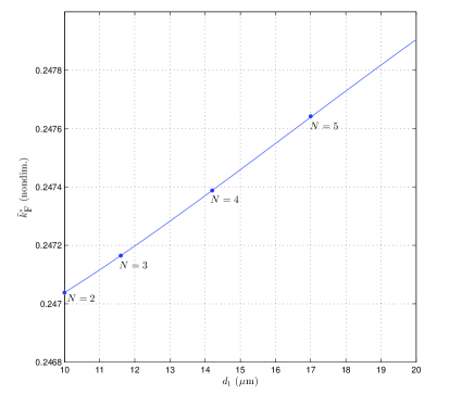
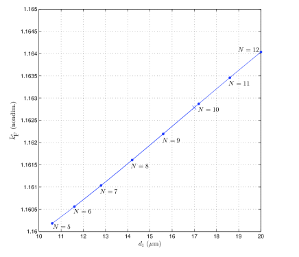
Figure 4.2 shows a numerical estimate for the lower bound k¯Fsubscriptsuperscript¯𝑘F\bar{k}^{*}_{\text{F}} in (4.17). For each fixed value of N𝑁N, N=2,,12𝑁212N=2,\dots,12, the curve indicates the value of k¯Fsubscriptsuperscript¯𝑘F\bar{k}^{*}_{\text{F}} as a functions of d1subscript𝑑1d_{1}, which is the distance between leader and follower. Since the scale of the curves is essentially different as N𝑁N changes, we present our results in two different pictures in Figures 4.2. Notice that the range of the distance d1subscript𝑑1d_{1} to be considered depends on N𝑁N according to (4.9) and (4.10) in Proposition 1: the starting point on the curve is marked by a “\bullet”, while the ending point is represented by d1=R4subscript𝑑1subscript𝑅4d_{1}=R_{4} for all N𝑁N. We have already observed that Γ(n)Γ𝑛\Gamma(n) can only obtain the values Γ(1)Γ1\Gamma(1) or Γ(3)Γ3\Gamma(3) according to Proposition 2. So, clearly, the curves for N=2,3,4𝑁234N=2,3,4 are overlapped (Figure 4.2 (a)), the same for N=6,,12𝑁612N=6,\dots,12 (Figure 4.2 (b)). For N=5𝑁5N=5 the curve starts in Figure 4.2 (b), with Γ(n)=Γ(3)Γ𝑛Γ3\Gamma(n)=\Gamma(3), until d117μmsubscript𝑑117𝜇md_{1}\approx 17\;\mu\text{m} (marker “×\times”), then Γ(n)Γ𝑛\Gamma(n) becomes Γ(1)Γ1\Gamma(1) and, for larger values of d1subscript𝑑1d_{1}, the curve continues in Figure 4.2 (a). For N=12𝑁12N=12 the right hand side of (4.17) assumes a single value in d1=R4subscript𝑑1subscript𝑅4d_{1}=R_{4} in Figure 4.2 (b).

Refer to caption
Refer to caption
Figure 4.2. Numerical plot of the lower bound k¯Fsubscriptsuperscript¯𝑘F\bar{k}^{*}_{\text{F}} in (4.17) as a function of d1subscript𝑑1d_{1}. The curve gives the lower bound for kFsubscriptsuperscript𝑘F{k}^{*}_{\text{F}} for a fixed N𝑁N and d1subscript𝑑1d_{1}. Since the scale of the curves is essentially different, we present in (a) the case N=2,3,4𝑁234N=2,3,4, in which the curves are overlapped, and similarly in (b) the case N=6,,12𝑁612N=6,\dots,12. The starting point on the curves is marked by “\bullet”, while the ending point is represented by d1=R4subscript𝑑1subscript𝑅4d_{1}=R_{4} for all N𝑁N. For N=5𝑁5N=5 the curve starts in (b) until d117μmsubscript𝑑117𝜇md_{1}\approx 17\;\mu\text{m} (marker “×\times”), then for larger values of d1subscript𝑑1d_{1} continues in (a). For N=12𝑁12N=12 the curve is reduced to a single value in d1=R4subscript𝑑1subscript𝑅4d_{1}=R_{4} in (b).

On the other hand, using again the numerical solution of f(𝐱)𝑓𝐱f(\mathbf{x}), the right hand side of (4.18) can be tabulated as N𝑁N changes. Its values are given in Table 1.

Table 1. Numerical values of the upper bound k¯Lsubscriptsuperscript¯𝑘L\bar{k}^{*}_{\text{L}} in (4.18) for N=2,,12𝑁212N=2,\dots,12. In practice fixing N𝑁N we have the upper bound of kLsubscriptsuperscript𝑘Lk^{*}_{\text{L}} for the existence of a steady N𝑁N-rosette.
N𝑁N k¯Lsubscriptsuperscript¯𝑘L\bar{k}^{*}_{\text{L}} (nondim.) N𝑁N k¯Lsubscriptsuperscript¯𝑘L\bar{k}^{*}_{\text{L}} (nondim.)
222 0.6707 8 1.8187
333 1.1580 9 1.8230
444 1.5146 10 1.8245
555 1.6987 11 1.8251
666 1.7769 12 1.8253
777 1.8073

Now, equation (4.1)1 becomes

j:𝐗j𝐁(𝐗L,R5)\{𝐗L}𝐊(𝐗j𝐗L)=𝟎,subscript:𝑗subscript𝐗𝑗\𝐁subscript𝐗Lsubscriptsuperscript𝑅5subscript𝐗L𝐊subscript𝐗𝑗subscript𝐗L0\displaystyle\sum_{j:\mathbf{X}_{j}\in\mathbf{B}(\mathbf{X}_{\text{L}},R^{*}_{5})\backslash\left\{\mathbf{X}_{\text{L}}\right\}}\mathbf{K}(\mathbf{X}_{j}-\mathbf{X}_{\text{L}})=\mathbf{0}, (4.19)
γf(𝐗i)¯+j:𝐗j𝐁(𝐗i,R4)\{𝐗i}𝐊(𝐗j𝐗i)=𝟎,i=1,,N,formulae-sequencesuperscript𝛾¯𝑓subscript𝐗𝑖subscript:𝑗subscript𝐗𝑗\𝐁subscript𝐗𝑖subscriptsuperscript𝑅4subscript𝐗𝑖𝐊subscript𝐗𝑗subscript𝐗𝑖0𝑖1𝑁\displaystyle\gamma^{*}\overline{\nabla f(\mathbf{X}_{i})}+\sum_{j:\mathbf{X}_{j}\in\mathbf{B}(\mathbf{X}_{i},R^{*}_{4})\backslash\left\{\mathbf{X}_{i}\right\}}\mathbf{K}(\mathbf{X}_{j}-\mathbf{X}_{i})=\mathbf{0},\quad i=1,\dots,N, (4.20)

respectively for the leader and for each follower. Here 𝐊𝐊\mathbf{K} contains only repulsion term:

𝐊(𝐗j𝐗i):=ωrep(1𝐗j𝐗i1R4)𝐗j𝐗i𝐗j𝐗i.assign𝐊subscript𝐗𝑗subscript𝐗𝑖subscriptsuperscript𝜔rep1normsubscript𝐗𝑗subscript𝐗𝑖1subscriptsuperscript𝑅4subscript𝐗𝑗subscript𝐗𝑖normsubscript𝐗𝑗subscript𝐗𝑖\displaystyle\mathbf{K}(\mathbf{X}_{j}-\mathbf{X}_{i}):=-\omega^{*}_{\text{rep}}\left(\frac{1}{||\mathbf{X}_{j}-\mathbf{X}_{i}||}-\frac{1}{R^{*}_{4}}\right)\frac{\mathbf{X}_{j}-\mathbf{X}_{i}}{||\mathbf{X}_{j}-\mathbf{X}_{i}||}.

For symmetry (4.19) is identically satisfied. Then in (4.20) f(𝐱,t)𝑓𝐱𝑡f(\mathbf{x},t) is given by (4.15) and (4.16), so in a circular domain ΩΩ\Omega we can write the same relation for all i𝑖i. For example, in relation to Figure 4.1 (b), we have

γyf(𝐗i)¯ωreph1(d1)ωreph2(N,d1)=0,superscript𝛾¯subscript𝑦𝑓subscript𝐗𝑖subscriptsuperscript𝜔repsubscript1subscriptsuperscript𝑑1subscriptsuperscript𝜔repsubscript2𝑁subscriptsuperscript𝑑10\displaystyle\gamma^{*}\overline{\partial_{y}f(\mathbf{X}_{i})}-\omega^{*}_{\text{rep}}h_{1}(d^{*}_{1})-\omega^{*}_{\text{rep}}h_{2}(N,d^{*}_{1})=0, (4.21)

in which ωreph1(d1)subscriptsuperscript𝜔repsubscript1subscriptsuperscript𝑑1\omega^{*}_{\text{rep}}h_{1}(d^{*}_{1}) represents the repulsion of the leader:

h1(d1):=1d11R4,assignsubscript1subscriptsuperscript𝑑11subscriptsuperscript𝑑11subscriptsuperscript𝑅4\displaystyle h_{1}(d^{*}_{1}):=\frac{1}{d^{*}_{1}}-\frac{1}{R^{*}_{4}},

d1=d1/Rsubscriptsuperscript𝑑1subscript𝑑1𝑅d^{*}_{1}=d_{1}/R is the nondimensional value of d1subscript𝑑1d_{1}, and ωreph2(N,d1)subscriptsuperscript𝜔repsubscript2𝑁subscriptsuperscript𝑑1\omega^{*}_{\text{rep}}h_{2}(N,d^{*}_{1}) is the possible repulsion of two adjoining followers according to (4.4) and Propositions 1, 2, namely:

h2(N,d1):={0,ifN4;2(12d1sinπ51R4)sinπ5,ifN=5d1R4<12sinπ5;0,ifN=512sinπ5d1R41;2(12d1sinπN1R4)sinπN,if6N12.assignsubscript2𝑁subscriptsuperscript𝑑1cases0if𝑁4212subscriptsuperscript𝑑1𝜋51subscriptsuperscript𝑅4𝜋5if𝑁5subscriptsuperscript𝑑1subscriptsuperscript𝑅412𝜋50if𝑁512𝜋5subscriptsuperscript𝑑1subscriptsuperscript𝑅41212subscriptsuperscript𝑑1𝜋𝑁1subscriptsuperscript𝑅4𝜋𝑁if6𝑁12\displaystyle h_{2}(N,d^{*}_{1}):=\left\{\begin{array}[]{lll}0,&\text{if}&N\leq 4;\\ 2\displaystyle\left(\frac{1}{2d^{*}_{1}\sin\frac{\pi}{5}}-\frac{1}{R^{*}_{4}}\right)\displaystyle\sin\frac{\pi}{5},&\text{if}&N=5\wedge\frac{d^{*}_{1}}{R^{*}_{4}}<\frac{1}{2\sin\frac{\pi}{5}};\\ 0,&\text{if}&N=5\wedge\frac{1}{2\sin\frac{\pi}{5}}\leq\frac{d^{*}_{1}}{R^{*}_{4}}\leq 1;\\ 2\displaystyle\left(\frac{1}{2d^{*}_{1}\sin\frac{\pi}{N}}-\frac{1}{R^{*}_{4}}\right)\displaystyle\sin\frac{\pi}{N},&\text{if}&6\leq N\leq 12.\end{array}\right. (4.26)

We remark that equation (4.21) is useful for two reasons. First, if we know an experimental value for the distance d1subscriptsuperscript𝑑1d^{*}_{1} we can obtain, fixing N𝑁N, the ratio ωrep/γsubscriptsuperscript𝜔repsuperscript𝛾\omega^{*}_{\text{rep}}/\gamma^{*} as a function of d1subscriptsuperscript𝑑1d^{*}_{1}:

ωrepγ=ΘN(d1):=yf(𝐗i)¯h1(d1)+h2(N,d1).subscriptsuperscript𝜔repsuperscript𝛾subscriptΘ𝑁subscriptsuperscript𝑑1assign¯subscript𝑦𝑓subscript𝐗𝑖subscript1subscriptsuperscript𝑑1subscript2𝑁subscriptsuperscript𝑑1\displaystyle\frac{\omega^{*}_{\text{rep}}}{\gamma^{*}}=\Theta_{N}(d^{*}_{1}):=\frac{\overline{\partial_{y}f(\mathbf{X}_{i})}}{h_{1}(d^{*}_{1})+h_{2}(N,d^{*}_{1})}. (4.27)

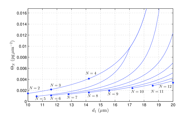
On the other hand, if ΘNsubscriptΘ𝑁\Theta_{N} is invertible, we can express d1subscriptsuperscript𝑑1d^{*}_{1} as a function of ωrepsubscriptsuperscript𝜔rep\omega^{*}_{\text{rep}} and γsuperscript𝛾\gamma^{*} that is the equilibrium distance for a N𝑁N-rosette fixed the physical parameters. Figure 4.3 represents a dimensional numerical plot of ΘNsubscriptΘ𝑁\Theta_{N} for N=2,,12𝑁212N=2,\dots,12. It shows that ΘNsubscriptΘ𝑁\Theta_{N} is monotone with respect to d1subscript𝑑1d_{1} for all N𝑁N, so that relation (4.27) is invertible. To obtain this plot the value of f(𝐱)𝑓𝐱f(\mathbf{x}) has been obtained numerically from (4.15) and (4.16) as previously described, fixing the same domain and the same parameters.

The domain of the curves, as in Figure 4.2, is given by (4.9) and (4.10); now it represents the admissible distances d1subscript𝑑1d_{1} for a N𝑁N-rosette, as N𝑁N changes. Symbol “\bullet” marks the origin of the curves. For N=2,3,4𝑁234N=2,3,4 the curves are overlapped (first line in the top) because for them h2=0subscript20h_{2}=0 (see (4.27) and (4.26)). For N=5𝑁5N=5 the curve coincide with the curve N=2,3,4𝑁234N=2,3,4 when h2subscript2h_{2} becomes zero. This happens about for d1>17μmsubscript𝑑117𝜇md_{1}>17\;\mu\text{m}, as we can see in (4.26)1,2,3. The curves corresponding to N=2,,6𝑁26N=2,\dots,6 have a vertical asymptote in d1=R4subscript𝑑1subscript𝑅4d_{1}=R_{4} where the functions h1subscript1h_{1} and h2subscript2h_{2} in (4.27) become zero. Conversely, for N=7,,12𝑁712N=7,\dots,12, ΘNsubscriptΘ𝑁\Theta_{N} is defined in d1=R4subscript𝑑1subscript𝑅4d_{1}=R_{4}. In particular for N=12𝑁12N=12, due to (4.10), the curve is reduced to a single value in d1=R4subscript𝑑1subscript𝑅4d_{1}=R_{4} given by Θ12(R4)subscriptΘ12subscript𝑅4\Theta_{12}(R_{4}) (marker point on the right).

Refer to caption
Figure 4.3. Dimensional numerical plot of ΘNsubscriptΘ𝑁\Theta_{N} for N=2,,12𝑁212N=2,\dots,12, that demonstrates that this function is monotone with respect to d1subscript𝑑1d_{1} and then invertible. The first three curves, for N=2,,4𝑁24N=2,\dots,4, coincide (first line in the top). Then, from the top to the bottom, we have the curves related to N=5,,11𝑁511N=5,\dots,11. For N=5𝑁5N=5 the curve goes to coincide with the first curve on the top about from d1>17μmsubscript𝑑117𝜇md_{1}>17\;\mu\text{m}. For N=12𝑁12N=12 the curve is reduced to a single value in d1=R4subscript𝑑1subscript𝑅4d_{1}=R_{4}. In practice fixing N𝑁N and d1subscript𝑑1d_{1} we have the value of ΘNsubscriptΘ𝑁\Theta_{N} that provides in (4.27) the ratio of the parameters ωrepsubscriptsuperscript𝜔rep\omega^{*}_{\text{rep}} and γsuperscript𝛾\gamma^{*}.

Typical values for N𝑁N and d1subscript𝑑1d_{1} (or d1subscriptsuperscript𝑑1d^{*}_{1}) to be used in (4.17), (4.18), and (4.27) will be given in Appendix A.

Now, in order to test numerically a steady N𝑁N-rosette, we perform a dynamic simulation of the model (3.36), as described in Section 5.1, with initial data given by a solution of the stationary system (4.1). In particular, we consider the spatial domain Ω=[0,200]×[0,200](μm2)Ω02000200𝜇superscriptm2\Omega=[0,200]\times[0,200]\;(\mu\text{m}^{2}) and the time interval [0,50](h)050h[0,50]\;(\text{h}), that is a typical time range used in the experimental observations [33]. Spatial and temporal discretizations are respectively Δx=Δy=0.2μmΔ𝑥Δ𝑦0.2𝜇m\Delta x=\Delta y=0.2\,\mu\text{m} and Δt=0.01hΔ𝑡0.01h\Delta t=0.01\,\text{h}. Initial data are set as follows:

𝐗i(0)=𝐗i0,subscript𝐗𝑖0subscript𝐗𝑖0\displaystyle\mathbf{X}_{i}(0)=\mathbf{X}_{i0}, (4.28)

𝐗i0subscript𝐗𝑖0\mathbf{X}_{i0} being a 888-rosette centered in 𝐗L(0)=(100,100)(μm)subscript𝐗L0100100𝜇m\mathbf{X}_{\text{L}}(0)=(100,100)\;(\mu\text{m}), with follower-leader distance fixed at d1=32Rsubscript𝑑132𝑅d_{1}=\frac{3}{2}R (see Appendix A and Figure 4.4 (a)),

𝐗˙i(0)=𝟎,subscript˙𝐗𝑖00\displaystyle\dot{\mathbf{X}}_{i}(0)=\mathbf{0}, (4.29)
f(𝐱,0)=f0(𝐱),𝑓𝐱0subscript𝑓0𝐱\displaystyle f(\mathbf{x},0)=f_{0}(\mathbf{x}), (4.30)

with f0(𝐱)subscript𝑓0𝐱f_{0}(\mathbf{x}) solution of equation (4.1)3 with homogeneous Neumann boundary condition in the same domain;

s(𝐱,0)=0,𝑠𝐱00\displaystyle s(\mathbf{x},0)=0, (4.31)

according to (4.1)4. The parameters used here are listed in Appendix A (see Tables LABEL:tab-param-dim, LABEL:tab-par-adim).

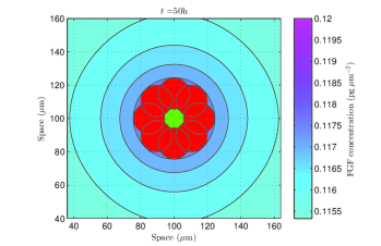
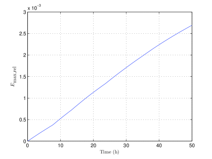
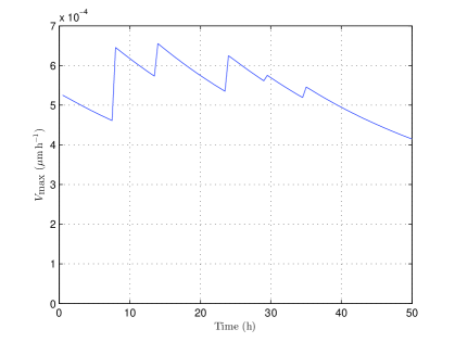
We see that our numerical results demonstrate that, with good approximation, the initial configuration stays constant in time. Figure 4.4 shows evolution in space of the dimensional solution at two different time steps: t=0h𝑡0ht=0\;\text{h} and t=50h𝑡50ht=50\;\text{h}. Green colour marks the leader cell (φi=1subscript𝜑𝑖1\varphi_{i}=1), and red colour marks a follower cell (φi=0subscript𝜑𝑖0\varphi_{i}=0). Contour plot in the background is related to the FGF signal concentration, while variable s(𝐱,t)𝑠𝐱𝑡s(\mathbf{x},t) is not shown. Figure 4.5 shows the evolution in time of the maximum relative error on the position, Emax,rel(t):=max1iNtot𝐗i(t)𝐗i0Rassignsubscript𝐸max,rel𝑡subscript1𝑖subscript𝑁totnormsubscript𝐗𝑖𝑡subscript𝐗𝑖0𝑅E_{\text{max,rel}}(t):=\frac{\max_{1\leq i\leq N_{\text{tot}}}\left\|\mathbf{X}_{i}(t)-\mathbf{X}_{i0}\right\|}{R}, and the maximum velocity Vmax(t):=max1iNtot𝐗˙i(t)assignsubscript𝑉max𝑡subscript1𝑖subscript𝑁totnormsubscript˙𝐗𝑖𝑡V_{\text{max}}(t):=\max_{1\leq i\leq N_{\text{tot}}}\left\|\dot{\mathbf{X}}_{i}(t)\right\|. Emax,relsubscript𝐸max,relE_{\text{max,rel}} suggests a deviation from the initial position in the order of 103superscript10310^{-3} times cell radius, while Vmaxsubscript𝑉maxV_{\text{max}} is in the order of 104superscript10410^{-4} μmh1𝜇msuperscripth1\mu\text{m}\,\text{h}^{-1}, which is very small with respect to the cell velocity during migration that is around 69μm/h69𝜇mh69\;\mu\text{m}/\text{h} [24].

Refer to caption
Refer to caption
Figure 4.4. Numerical simulation of a steady solution given by a 888-rosette. (a)-(b) are related respectively to the dimensional plot at two different time steps: t=0h𝑡0ht=0\;\text{h} and t=50h𝑡50ht=50\;\text{h}. System (3.36) is solved as described in Section 5.1 in Ω=[0,200]×[0,200](μm2)Ω02000200𝜇superscriptm2\Omega=[0,200]\times[0,200]\;(\mu\text{m}^{2}) (plot refers only to a part of the domain) and in [0,50](h)050h[0,50]\;(\text{h}). Spatial and temporal discretization is set to Δx=Δy=0.2μmΔ𝑥Δ𝑦0.2𝜇m\Delta x=\Delta y=0.2\;\mu\text{m} and Δt=0.01hΔ𝑡0.01h\Delta t=0.01\;\text{h}. Initial data are given by (4.28)–(4.31). The parameters used here are listed in Appendix A. Green colour (\bullet) marks the leader cell, red colour (\bullet) a follower cell, contour plot in the background is the FGF signal concentration. Variable s(𝐱,t)𝑠𝐱𝑡s(\mathbf{x},t) is not shown.
Refer to caption
Refer to caption
Figure 4.5. Numerical assessment of a steady 888-rosette.(a) Plot in time of the maximum relative error Emax,rel(t)subscript𝐸max,rel𝑡E_{\text{max,rel}}(t). (b) Plot of the maximum velocity Vmax(t)subscript𝑉max𝑡V_{\text{max}}(t).

Now the stability of a N𝑁N-rosette will be numerically investigated. Starting from the previous numerical test we perform a dynamic simulation perturbing the initial equilibrium configuration of the 888-rosette. Namely, each center of a follower cell is translated of a ray vector whose magnitude and direction are random number in the interval [0,5](μm)05𝜇m[0,5]\;(\mu\text{m}) and [0,2π]02𝜋[0,2\pi]. Spatial domain and parameters are the same as in the previous simulation, while the time range is set to [0,60](h)060h[0,60]\;(\text{h}).

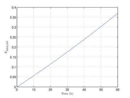
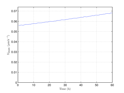
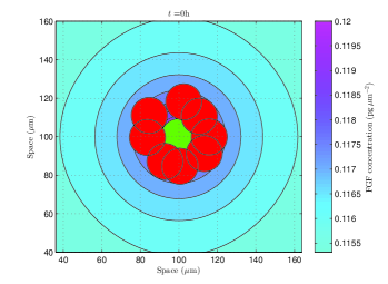
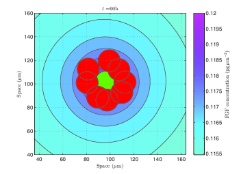
Figure 4.6 shows the evolution in space of the dimensional solution at two time steps: t=0h𝑡0ht=0\,\text{h} and t=60h𝑡60ht=60\,\text{h}. Colour convention is the same as Figure 4.6. Figure 4.7 shows the evolution in time of the maximum relative error on the position Emax,rel(t)subscript𝐸max,rel𝑡E_{\text{max,rel}}(t) and the maximum velocity Vmax(t)subscript𝑉max𝑡V_{\text{max}}(t). Emax,relsubscript𝐸max,relE_{\text{max,rel}} indicates a deviation from the initial position in the order of 101superscript10110^{-1} times cell radius, and also Vmaxsubscript𝑉maxV_{\text{max}} is small, being in the order of 102superscript10210^{-2} μmh1𝜇msuperscripth1\mu\text{m}\,\text{h}^{-1}. Our data demonstrate as the equilibrium configuration of our 888-rosette is stable. Furthermore, numerical simulations show that similar results can hold also if N8𝑁8N\neq 8, for instance for N=5𝑁5N=5 or 101010. We note that in a physically reasonable time range we do not observe the asymptotic stability of the rosette structures, which is actually not expected, but just the simple stability.
Refer to caption
Refer to caption
Figure 4.6. Numerical assessment of stability of a 888-rosette. (a)-(b) are related respectively to the dimensional plot at t=0h𝑡0ht=0\,\text{h} and t=60h𝑡60ht=60\,\text{h}. System (3.36) is solved as described in Section 5.1 in Ω=[0,200]×[0,200](μm2)Ω02000200𝜇superscriptm2\Omega=[0,200]\times[0,200]\;(\mu\text{m}^{2}) (plot refers only to a part of the domain) and in [0,50](h)050h[0,50]\;(\text{h}). Spatial and temporal discretization is the same as in Figure (4.4). Initial data are given by a perturbation of positions (4.28), and by (4.29)–(4.31). The parameters used here are listed in Appendix A. Green colour (\bullet) marks the leader cell, red colour (\bullet) a follower cell, contour plot in the background is the FGF signal concentration. Variable s(𝐱,t)𝑠𝐱𝑡s(\mathbf{x},t) is not shown.
Refer to caption
Refer to caption
Figure 4.7. Numerical assessment of stability of a 888-rosette. (a) Plot in time of the maximum relative error Emax,rel(t)subscript𝐸max,rel𝑡E_{\text{max,rel}}(t). (b) Plot of the maximum velocity Vmax(t)subscript𝑉max𝑡V_{\text{max}}(t).

5. Dynamic simulations

5.1. Numerical methods

All the numerical tests in the paper employ a 2D finite difference scheme with a uniform spatial and temporal grid.

About system (3.36), the equation for 𝐗¨¨𝐗\ddot{\mathbf{X}} is reduced to the first order system

{𝐘i˙=αW𝐁(𝐗i,R¯)s(𝐱,t)wi(𝐱)𝑑𝐱+γ(1φi)W𝐁(𝐗i,R¯)f(𝐱,t)wi(𝐱)𝑑𝐱+1N¯ij:𝐗j𝐁(𝐗i,R1)\{𝐗i}𝐇(𝐘j𝐘i)+j:𝐗j𝐁(𝐗i,R5)\{𝐗i}𝐊(𝐗j𝐗i)[μF+(μLμF)φi]𝐘i,𝐗i˙=𝐘i.cases˙subscript𝐘𝑖absentsuperscript𝛼𝑊subscript𝐁subscript𝐗𝑖superscript¯𝑅𝑠𝐱𝑡subscript𝑤𝑖𝐱differential-d𝐱superscript𝛾1subscript𝜑𝑖𝑊subscript𝐁subscript𝐗𝑖superscript¯𝑅𝑓𝐱𝑡subscript𝑤𝑖𝐱differential-d𝐱missing-subexpressionmissing-subexpressionmissing-subexpression1subscript¯𝑁𝑖subscript:𝑗subscript𝐗𝑗\𝐁subscript𝐗𝑖subscriptsuperscript𝑅1subscript𝐗𝑖𝐇subscript𝐘𝑗subscript𝐘𝑖subscript:𝑗subscript𝐗𝑗\𝐁subscript𝐗𝑖subscriptsuperscript𝑅5subscript𝐗𝑖𝐊subscript𝐗𝑗subscript𝐗𝑖delimited-[]subscriptsuperscript𝜇Fsubscriptsuperscript𝜇Lsubscriptsuperscript𝜇Fsubscript𝜑𝑖subscript𝐘𝑖missing-subexpressionmissing-subexpression˙subscript𝐗𝑖absentsubscript𝐘𝑖\begin{split}\left\{\begin{array}[]{ll}\dot{\mathbf{Y}_{i}}&=\displaystyle\frac{\alpha^{*}}{W}\int_{\mathbf{B}(\mathbf{X}_{i},\bar{R}^{*})}\nabla s(\mathbf{x},t)w_{i}(\mathbf{x})\,d\mathbf{x}+\displaystyle\frac{\gamma^{*}(1-\varphi_{i})}{W}\int_{\mathbf{B}(\mathbf{X}_{i},\bar{R}^{*})}\nabla f(\mathbf{x},t)w_{i}(\mathbf{x})\,d\mathbf{x}\\ \\ &+\displaystyle\frac{1}{\bar{N}_{i}}\sum_{j:\mathbf{X}_{j}\in\mathbf{B}(\mathbf{X}_{i},R^{*}_{1})\backslash\left\{\mathbf{X}_{i}\right\}}\mathbf{H}(\mathbf{Y}_{j}-\mathbf{Y}_{i})+\sum_{j:\mathbf{X}_{j}\in\mathbf{B}(\mathbf{X}_{i},R^{*}_{5})\backslash\left\{\mathbf{X}_{i}\right\}}\mathbf{K}(\mathbf{X}_{j}-\mathbf{X}_{i})-\left[\mu^{*}_{\text{F}}+(\mu^{*}_{\text{L}}-\mu^{*}_{\text{F}})\varphi_{i}\right]\mathbf{Y}_{i},\\ \\ \dot{\mathbf{X}_{i}}&=\mathbf{Y}_{i}.\end{array}\right.\end{split} (5.1)

Then equation (5.1)1 is discretized with the backward Euler method, putting totally implicit the terms in 𝐘isubscript𝐘𝑖\mathbf{Y}_{i} and 𝐘jsubscript𝐘𝑗\mathbf{Y}_{j} at the right hand side, while totally explicit the other addends. Equation (5.1)2 is solved with the forward Euler method.

About equation (3.36)3 we use a classical exponential transformation in order to eliminate the stiff term ηfsuperscript𝜂𝑓-\eta^{*}f, and then we apply a central difference scheme in space and the parabolic Crank-Nicolson scheme in time, subject to zero flux boundary conditions. In practice, in the numerical simulations we choose the domain size sufficiently large that over the time period of interest have a negligible impact on the solution.

Finally in equation (3.36)4 the explicit Euler method is employed.

5.2. Numerical tests

Now we simulate the zebrafish lateral line growth in a two-dimensional space, during about 20h20h20\;\text{h}. Using the numerical method proposed in Section 5.1 we solve system (3.36) in a domain Ω=[0,5000]×[0,1240](μm2)Ω0500001240𝜇superscriptm2\Omega=[0,5000]\times[0,1240]\;(\mu\text{m}^{2}), with a spatial and temporal discretization given respectively by Δx=Δy=5μmΔ𝑥Δ𝑦5𝜇m\Delta x=\Delta y=5\,\mu\text{m} and Δt=0.001hΔ𝑡0.001h\Delta t=0.001\,\text{h}. Parameters values used here are listed in Appendix A (Tables LABEL:tab-param-dim, LABEL:tab-par-adim). Initial and boundary conditions are given by (3.24)–(3.30). In particular, as initial datum 𝐗i(0)subscript𝐗𝑖0\mathbf{X}_{i}(0), we set 90 cells equally distributed in the stripe [600,1180]×[600,640](μm2)6001180600640𝜇superscriptm2[600,1180]\times[600,640]\;(\mu\text{m}^{2}) at a distance between their centers of 17μm17𝜇m17\;\mu\text{m}, and then randomized around their position with radius in the range [0,3](μm)03𝜇m[0,3]\;(\mu\text{m}) and angles in [0,2π]02𝜋[0,2\pi] (Figure 5.1 (a)). As initial condition s(𝐱,0)𝑠𝐱0s(\mathbf{x},0) in equation (3.29) we fix c1=838μmsubscript𝑐1838𝜇mc_{1}=838\;\mu\text{m} (the inflection point of the tanh\tanh is about at the middle of the primordium), c2=200μmsubscript𝑐2200𝜇mc_{2}=200\;\mu\text{m}, and [a¯,b¯]=[600,5000](μm)¯𝑎¯𝑏6005000𝜇m[\bar{a},\bar{b}]=[600,5000]\;(\mu\text{m}). Then in (3.30) and (3.35) we choose l=20μm𝑙20𝜇ml=20\;\mu\text{m} and ε=10μm𝜀10𝜇m\varepsilon=10\;\mu\text{m}.

Figures 5.1, 5.2 show the numerical simulations of the lateral line evolution as described above at different time steps. As usual, green colour marks leader cells (φi=1subscript𝜑𝑖1\varphi_{i}=1), and red colour the followers (φi=0subscript𝜑𝑖0\varphi_{i}=0). Contour plot in the background to FGF signal, while variable s(𝐱,t)𝑠𝐱𝑡s(\mathbf{x},t) is not shown. In our simulation we can observe, in the first few hours after migration starts, the leader-to-follower transition of some cells in the trailing region of the primordium, up to about t=6.5h𝑡6.5ht=6.5\;\text{h} when a first rosette starts detaching (Figures 5.1 (b)). This is consistent with the experimental results presented in the supplementary material in [33, 24], that shows a time of about 36363\text{--}6 h for the first rosette separation. Figures 5.1 (c) shows the formation of a second rosette in the new trailing region, meanwhile in the first rosette the lateral inhibition process is completed leaving two leader cells. Then in the next time steps, until about t=20h𝑡20ht=20\;\text{h}, we observe the detachment of the other two rosettes (Figure 5.2).
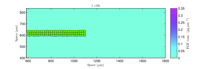
Refer to caption
Refer to caption
Refer to caption
Figure 5.1. Numerical simulation of the lateral line growth at five different time steps: t=0,6.47,10.15h𝑡06.4710.15ht=0,6.47,10.15\;\text{h}, next two time steps t=15.64,19h𝑡15.6419ht=15.64,19\;\text{h} are plotted in Figure 5.2). System (3.36) is solved in the domain Ω=[0,5000]×[0,1240](μm2)Ω0500001240𝜇superscriptm2\Omega=[0,5000]\times[0,1240]\;(\mu\text{m}^{2}) (plot shows only a part of the domain), with a spatial and temporal discretization given respectively by Δx=Δy=5μmΔ𝑥Δ𝑦5𝜇m\Delta x=\Delta y=5\,\mu\text{m} and Δt=0.001hΔ𝑡0.001h\Delta t=0.001\,\text{h}. Parameters values used here are listed in Appendix A. Initial and boundary conditions are given by (3.24), (3.25), (3.26), and (3.28). In particular, about initial condition s(𝐱,0)𝑠𝐱0s(\mathbf{x},0), in equation (3.29) we have fixed c1=838μmsubscript𝑐1838𝜇mc_{1}=838\;\mu\text{m}, c2=200μmsubscript𝑐2200𝜇mc_{2}=200\;\mu\text{m}, and [a¯,b¯]=[600,5000](μm)¯𝑎¯𝑏6005000𝜇m[\bar{a},\bar{b}]=[600,5000]\;(\mu\text{m}). Then in (3.30) and (3.35) we have chosen l=20μm𝑙20𝜇ml=20\;\mu\text{m} and ε=10μm𝜀10𝜇m\varepsilon=10\;\mu\text{m}. Green colour (\bullet) is for leader cells, red colour (\bullet) for the followers. Contour plot in the background indicates the FGF concentration, while variable s(𝐱,t)𝑠𝐱𝑡s(\mathbf{x},t) is not shown.
Refer to caption
Refer to caption
Figure 5.2. Continuation of Figure 5.1. Numerical simulation of the lateral line growth at time steps: t=15.64,19h𝑡15.6419ht=15.64,19\;\text{h}.

In Figure 5.3 we have plotted migration velocity of the tip of the primordium versus time for 6 hours. Taking into account the velocity of 69μm/h69𝜇mh69\;\mu\text{m}/\text{h} given in [24], we can state a good concordance of our data. Moreover we observe a decrease in velocity in correspondence with the formation of the first rosette. This is substantially comparable with the velocity plot shown in [24] in Figure 4 (c).

Finally, from the numerical simulations, we observe a flocking behavior in cell migration, according to the results shown in [9, 17] for Cucker-Smale term (3.8), although in our model other effects are involved, as chemotaxis and adhesion-repulsion terms. We recall that in [9] flocking behaviour occurs unconditionally when the power of the denominator in (3.10) is less than 1/2, and conditionally if this power is equal or greater than 1/2. If we consider only the equations (3.8)–(3.10) we are in the case of conditional flocking, and the flocking behaviour is ensured by the initial data (3.24).
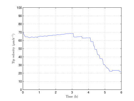
Refer to caption
Figure 5.3. Numerical dimensional plot of the velocity of tip of the primordium during migration versus time.

6. Conclusions

We have proposed in this paper a discrete in continuous mathematical model describing the formation of the lateral line in the zebrafish primordium. Under suitable hypothesis, we have shown that our model admits particular biologically relevant steady solutions. They corresponds to the formation of neuromasts along the two flanks of the embryo. Then their stability has been tested numerically. Finally, the dynamical model has been tested by 2D numerical simulations and the results have been compared with some experimental observations.

Clearly we remark that the model proposed here presents some limits. Firstly, cells are supposed to be all equally circular, so that deformation effects are neglected. On the other hand they can be partially recovered introducing influence radii. Secondly, only a limited number of biological interactions have been modeled, and this in a time range starting with the beginning of the migration of the primordium. For example, biological phenomena occurring in the next few hours post-fertilization, or in the time after the rosettes deposition have not been taken into account. However we have followed the framework of the studies [33, 24], and a good concordance with the experimental data can be inferred.

Finally, we remark that with respect to [33, 24] we have introduced other mechanisms to obtain the global migration and the neuromast formation, as lateral inhibition, alignment, and adhesion-repulsion effects. It would be interesting to have experimental evidence in this regard.

Appendix A Parameters estimates

About the choice of the parameters of the model, we point out that while some values can be found or estimated from the biological or modelling literature, the others have been obtained by numerical data fitting or using some relations provided by the stationary model.

Tables LABEL:tab-param-dim and LABEL:tab-par-adim summarize respectively the values of the dimensional and nondimensional parameters. In the case of a range of variability for a parameter, the selected value, used in the simulations, is put in brackets. Finally, the last column in Table LABEL:tab-param-dim specifies the references for the provided data.

Now we will make some comments in this regard. Firstly, cell radius R𝑅R is fixed to 10μm10𝜇m10\;\mu\mbox{m} starting from the experimental data in [24]. Radii R¯¯𝑅\bar{R}, R1subscript𝑅1R_{1}, R2subscript𝑅2R_{2}, are chosen to be equal to 20μm20𝜇m20\;\mu\mbox{m}, taking into account a possible effect of cell extensions. Radius R3subscript𝑅3R_{3}, concerning with the range of production or degradation of a chemical signaling, is set to be equal to R𝑅R, because we think to a source or a drain defined by the dimension of a single cell. For R4subscript𝑅4R_{4} and R5subscript𝑅5R_{5} we fix respectively the values 20μm20𝜇m20\;\mu\mbox{m} and 25μm25𝜇m25\;\mu\mbox{m}. First value provides a repulsion force when two cells start to be overlapped (see equation (3.15)1), second values implies an adhesion force in the spatial radial range 20–25 μm𝜇m\mu\mbox{m}. The values of α𝛼\alpha, βLsubscript𝛽L\beta_{\text{L}}, βFsubscript𝛽F\beta_{\text{F}}, γ𝛾\gamma, ωadh,Fsubscript𝜔adh,F\omega_{\text{adh,F}}, μFsubscript𝜇F\mu_{\text{F}}, δ/λ𝛿𝜆\delta/\lambda, and σ𝜎\sigma, are obtained by a numerical data fitting on the respective dimensionless values, in order to obtain in the simulations a cell migration velocity and a neuromasts formation consistent with the experimental results.

About the information on the parameters arising from the stationary model, we refer to formulas (4.17), (4.18), (4.27), Table 1, and Figures 4.2, 4.3. The first two relations give us a limitation for kF:=kF/λassignsubscriptsuperscript𝑘Fsubscript𝑘F𝜆k^{*}_{\text{F}}:=k_{\text{F}}/\lambda and kL:=kL/λassignsubscriptsuperscript𝑘Lsubscript𝑘L𝜆k^{*}_{\text{L}}:=k_{\text{L}}/\lambda, while the third one provides a value of ωrepsubscript𝜔rep\omega_{\text{rep}} when we have fixed γ𝛾\gamma by a numerical choice. Namely, the right hand side of these equations depend on N𝑁N and d1subscriptsuperscript𝑑1d^{*}_{1} once the other parameters are chosen. So, to obtain the values in Tables LABEL:tab-param-dim, LABEL:tab-par-adim we have fixed for an example N=8𝑁8N=8 and d1=3/2Rsubscriptsuperscript𝑑132superscript𝑅d^{*}_{1}=3/2R^{*}. They represent reasonable values under the experimental observations in [33] and [24].

Then a value for ξ𝜉\xi is obtained from the respective nondimensional value ξsuperscript𝜉\xi^{*} in order to have fmax=1subscriptsuperscript𝑓1f^{*}_{\max}=1 setting a single leader cell in our domain. Finally other constants are estimable from data available in literature: smaxsubscript𝑠s_{\max}, from [23]; fmaxsubscript𝑓f_{\max}, from [40]; ωadh,Lsubscript𝜔adh,L\omega_{\text{adh,L}}, from [4]; μLsubscript𝜇L\mu_{\text{L}}, from [36]; D𝐷D, from [41, 13] and a phenomenological formula in [20]; η𝜂\eta from [3, 25], using the FGF half-life estimates.

Table 2. Estimates of physical parameter values.
Parameter Definition Value or range (used value) Source
R𝑅R cell radius 10 μm𝜇m\mu\text{m} [24]
  R¯¯𝑅\bar{R} detection radius of chemicals 20 μm𝜇m\mu\text{m} biological assumption
R1subscript𝑅1R_{1} detection radius of cellular alignment 20 μm𝜇m\mu\text{m} biological assumption
R2subscript𝑅2R_{2} detection radius of lateral inhibition 20 μm𝜇m\mu\text{m} biological assumption
R3subscript𝑅3R_{3} radius of production/degradation of chemicals 10 μm𝜇m\mu\text{m} biological assumption
R4subscript𝑅4R_{4} radius of action of repulsion between cells 20 μm𝜇m\mu\text{m} biological assumption
R5subscript𝑅5R_{5} radius of action of adhesion between cells 25 μm𝜇m\mu\text{m} biological assumption
T characteristic time 1/3600h13600h1/3600\,\text{h} [36]
smaxsubscript𝑠s_{\max} maximum concentration of SDF-1a 3.6×1086.5×1083.6superscript1086.5superscript1083.6\times 10^{-8}\text{--}6.5\times 10^{-8} (2.5×10⁸)pgμm22.5superscript108pg𝜇superscriptm2(2.5\times 10^{-8})\;\text{pg}\,\mu\text{m}^{-2} [23]
fmaxsubscript𝑓f_{\max} maximum concentration of FGF 1×101(1.2×101)pgμm21superscript1011.2superscript101pg𝜇superscriptm21\times 10^{-1}\text{--}(1.2\times 10^{-1})\;\text{pg}\,\mu\text{m}^{-2} [40]
Γ0subscriptΓ0\Gamma_{0} constant in function (3.17) 10 nondim. assumed
α𝛼\alpha coefficient of SDF-1a haptotactic effect per unit mass 1.31×1027μm4h2pg11.31superscript1027𝜇superscriptm4superscripth2superscriptpg11.31\times 10^{27}\;\mu\text{m}^{4}\,\text{h}^{-2}\,\text{pg}^{-1} assumed
βLsubscript𝛽L\beta_{\text{L}} coefficient of cell flocking per unit mass for a leader cell 5×10²⁰h15superscript1020superscripth15\times 10^{20}\;\text{h}^{-1} assumed
βFsubscript𝛽F\beta_{\text{F}} coefficient of cell flocking per unit mass for a follower cell 5×10¹⁸h15superscript1018superscripth15\times 10^{18}\;\text{h}^{-1} assumed
γ𝛾\gamma coefficient of attraction toward FGF source per unit mass 1.08×1020μm4h2pg11.08superscript1020𝜇superscriptm4superscripth2superscriptpg11.08\times 10^{20}\;\mu\text{m}^{4}\,\text{h}^{-2}\,\text{pg}^{-1} assumed
ωrepsubscript𝜔rep\omega_{\text{rep}} coefficient of repulsion per unit mass 2.03×1017μm2h22.03superscript1017𝜇superscriptm2superscripth22.03\times 10^{17}\;\mu\text{m}^{2}\,\text{h}^{-2} from steady model, formula (4.27)
ωadh,Lsubscript𝜔adh,L\omega_{\text{adh,L}} elastic constant per unit mass for a leader cell 1.296×10141.296×10191.296superscript10141.296superscript10191.296\times 10^{14}\text{--}1.296\times 10^{19} (5.5×10¹⁶)h25.5superscript1016superscripth2(5.5\times 10^{16})\;\text{h}^{-2} [4]
ωadh,Fsubscript𝜔adh,F\omega_{\text{adh,F}} elastic constant per unit mass for a follower cell 1.296×10121.296×10171.296superscript10121.296superscript10171.296\times 10^{12}\text{--}1.296\times 10^{17} (5.5×10¹⁴)h25.5superscript1014superscripth2(5.5\times 10^{14})\;\text{h}^{-2} assumed
μLsubscript𝜇L\mu_{\text{L}} damping coefficient for a leader cell per unit mass (5.82×10¹⁴)5.82×10155.82superscript10145.82superscript1015(5.82\times 10^{14})\text{--}5.82\times 10^{15} h1superscripth1\text{h}^{-1} [36]
μFsubscript𝜇F\mu_{\text{F}} damping coefficient for a follower cell per unit mass (8×10¹⁵)8×10¹⁶h18superscript10158superscript1016superscripth1(8\times 10^{15})\text{--}8\times 10^{16}\;\text{h}^{-1} assumed
δ/λ𝛿𝜆\delta/\lambda ratio of coefficient of sensibility to SDF-1a and coefficient of lateral inhibition 1.12×1091.12superscript1091.12\times 10^{9} pg1μm2superscriptpg1𝜇superscriptm2\;\text{pg}^{-1}\,\mu\text{m}^{2} assumed
kL/λsubscript𝑘L𝜆k_{\text{L}}/\lambda ratio of coefficient of sensibility to FGF signal for a leader cell and coefficient of lateral inhibition <1.8187absent1.8187<1.8187 (1.7) nondim. from steady model, formula (4.18)
kF/λsubscript𝑘F𝜆k_{\text{F}}/\lambda ratio of coefficient of sensibility to FGF signal for a follower cell and coefficient of lateral inhibition 1.1619absent1.1619\geq 1.1619 (17) nondim. from steady model, formula (4.17)
D𝐷D diffusion coefficient 69985–84184 (78950) μm2s1𝜇superscriptm2superscripts1\mu\text{m}^{2}\,\text{s}^{-1} [20, 13, 41]
ξ𝜉\xi coefficient of production of FGF 2.9592pgμm2h12.9592pg𝜇superscriptm2superscripth12.9592\;\text{pg}\,\mu\text{m}^{-2}\,\text{h}^{-1} assumed
η𝜂\eta degradation constant of FGF 0.09–0.69 (0.2) h1superscripth1\text{h}^{-1} [3, 25]
σ𝜎\sigma degradation constant of SDF-1a 0.6 h1superscripth1\text{h}^{-1} assumed
Table 3. Estimates of dimensionless parameter values.
Parameter Definition Value or range (used value)
  R¯superscript¯𝑅\bar{R}^{*} R¯/R¯𝑅𝑅\bar{R}/R 2
  R1subscriptsuperscript𝑅1R^{*}_{1} R1/Rsubscript𝑅1𝑅R_{1}/R 2
  R2subscriptsuperscript𝑅2R^{*}_{2} R2/Rsubscript𝑅2𝑅R_{2}/R 2
  R3subscriptsuperscript𝑅3R^{*}_{3} R3/Rsubscript𝑅3𝑅R_{3}/R 1
  R4subscriptsuperscript𝑅4R^{*}_{4} R4/Rsubscript𝑅4𝑅R_{4}/R 2
  R5subscriptsuperscript𝑅5R^{*}_{5} R5/Rsubscript𝑅5𝑅R_{5}/R 2,5
  Γ0subscriptΓ0\Gamma_{0} Γ0subscriptΓ0\Gamma_{0} 10
  αsuperscript𝛼\alpha^{*} αsmaxT2/R2𝛼subscript𝑠superscript𝑇2superscript𝑅2\alpha s_{\max}T^{2}/R^{2} 2.53×10102.53superscript10102.53\times 10^{10}
  βLsuperscriptsubscript𝛽L\beta_{\text{L}}^{*} βLTsubscript𝛽L𝑇\beta_{\text{L}}T 1.39×10171.39superscript10171.39\times 10^{17}
  βFsuperscriptsubscript𝛽F\beta_{\text{F}}^{*} βFTsubscript𝛽F𝑇\beta_{\text{F}}T 1.39×10151.39superscript10151.39\times 10^{15}
  γsuperscript𝛾\gamma^{*} γfmaxT2/R2𝛾subscript𝑓superscript𝑇2superscript𝑅2\gamma f_{\max}T^{2}/R^{2} 1010superscript101010^{10}
  ωrepsubscriptsuperscript𝜔rep\omega^{*}_{\text{rep}} ωrepT2/R2subscript𝜔repsuperscript𝑇2superscript𝑅2\omega_{\text{rep}}T^{2}/R^{2} 1.57×1081.57superscript1081.57\times 10^{8}
  ωadh,Lsubscriptsuperscript𝜔adh,L\omega^{*}_{\text{adh,L}} ωadh,LT2subscript𝜔adh,Lsuperscript𝑇2\omega_{\text{adh,L}}T^{2} 107superscript10710^{7}1012superscript101210^{12} (4.24×1094.24superscript1094.24\times 10^{9})
  ωadh,Fsubscriptsuperscript𝜔adh,F\omega^{*}_{\text{adh,F}} ωadh,FT2subscript𝜔adh,Fsuperscript𝑇2\omega_{\text{adh,F}}T^{2} 105superscript10510^{5}1010superscript101010^{10} (4.24×1074.24superscript1074.24\times 10^{7})
  μLsubscriptsuperscript𝜇L\mu^{*}_{\text{L}} μLTsubscript𝜇L𝑇\mu_{\text{L}}T (1.62×10¹¹)1.62superscript1011(1.62\times 10^{11})1.62×10121.62superscript10121.62\times 10^{12}
  μFsubscriptsuperscript𝜇F\mu^{*}_{\text{F}} μFTsubscript𝜇F𝑇\mu_{\text{F}}T (2.22×10¹²(2.22\times 10^{12})–2.21×10132.21superscript10132.21\times 10^{13}
  δsuperscript𝛿\delta^{*} δsmax/λ𝛿subscript𝑠𝜆\delta s_{\max}/\lambda 28
  kLsubscriptsuperscript𝑘Lk^{*}_{\text{L}} kL/λsubscript𝑘L𝜆k_{\text{L}}/\lambda <1.8187absent1.8187<1.8187 (1.7)
  kFsubscriptsuperscript𝑘Fk^{*}_{\text{F}} kF/λsubscript𝑘F𝜆k_{\text{F}}/\lambda 1.1619absent1.1619\geq 1.1619 (17)
  Dsuperscript𝐷D^{*} DT/R2𝐷𝑇superscript𝑅2DT/R^{2} 0.1944–0.2338 (0.2193)
  ξsuperscript𝜉\xi^{*} ξT/fmax𝜉𝑇subscript𝑓\xi T/f_{\max} 0.0069
  ηsuperscript𝜂\eta^{*} ηT𝜂𝑇\eta T 2.5×1052.5superscript1052.5\times 10^{-5}1.92×1041.92superscript1041.92\times 10^{-4} (5.56×1055.56superscript1055.56\times 10^{-5})
  σsuperscript𝜎\sigma^{*} σT𝜎𝑇\sigma T 1.67×1041.67superscript1041.67\times 10^{-4}

Acknowledgements

We thank Andrea Tosin for some useful discussions and suggestions. The research leading to these results has received funding from the European Union Seventh Framework Programme [FP7/2007-2013] under grant agreement n. 257462 HYCON2 Network of excellence. This work has also been partially supported by the PRIN project 2008-2009 “Equazioni iperboliche non lineari e fluidodinamica”.

References

  • [1] G. Albi, L. Pareschi, Modeling self-organized systems interacting with few individuals: From microscopic to macroscopic dynamics, Applied Mathematics Letters 26 (4), 397–401 (2013).
  • [2] P. V. Bayly, L. A. Taber, A. E. Carlsson, Damped and persistent oscillations in a simple model of cell crawling, Journal of the Royal Society Interface 9 (71), 1241–1253 (2012).
  • [3] A. Beenken, M. Mohammadi, The FGF family: biology, pathophysiology and therapy, Nature Reviews Drug Discovery 8 (3), 235–253 (2009).
  • [4] G. I. Bell, M. Dembo, P. Bongrand, Cell adhesion. Competition between nonspecific repulsion and specific bonding, Biophys. Journal 45(6), 1051–1064 (1984).
  • [5] R. T. Böttcher, C. Niehrs, Fibroblast Growth Factor Signaling during Early Vertebrate Development, Endocrine Reviews 26 (1), 63–77 (2005).
  • [6] A. B. Chitnis, D. D. Nogare, M. Matsuda, Building the Posterior Lateral Line System in Zebrafish, Developmental Neurobiology 72 (3), 234–255 (2012).
  • [7] S. Coombs, S. V. Netten, The Hydrodynamics and Structural Mechanics of the Lateral Line System, Fish Physiology 23, 103–139 (2005).
  • [8] E. Cristiani, B. Piccoli, A. Tosin, Multiscale modeling of granular flows with application to crowd dynamics., Multiscale Modeling & Simulation 9 (1), 155–182 (2011).
  • [9] F. Cucker, S. Smale, Emergent Behavior in Flocks, IEEE Transactions On Automatic Control 52 (5), 852–862 (2007).
  • [10] M. R. D’Orsogna, Y. L. Chuang, A. L. Bertozzi, L. S. Chayes, Self-Propelled Particles with Soft-Core Interactions: Patterns, Stability, and Collapse, Physical Review Letters 96 (10), 104302 (2006).
  • [11] B. W. Draper, P. A. Morcos, C. B. Kimmel, Inhibition of Zebrafish fgf8 Pre-mRNA Splicing With Morpholino Oligos: A Quantifiable Method for Gene Knockdown, Genesis 30, 154–156 (2001).
  • [12] M. Eisenbach, J. W. Lengeler, Chemotaxis, Imperial College Press (2004).
  • [13] R. J. Filion, A. S. Popel, Intracoronary administration of FGF-2: a computational model of myocardial deposition and retention, Am. J. Physiol. Heart Circ. Physiol. 288 (1), H263–H279 (2005).
  • [14] M. F. Fournier, R. Sauser, D. Ambrosi, J.-J. Meister, A. B. Verkhovsky, Force transmission in migrating cells, Journal of Cell Biology 188 (2), 287–297 (2010).
  • [15] A. Ghysen, C. D. Chaudière, Development of the zebrafish lateral line, Current Opinion in Neurobiology 14, 67–73 (2004).
  • [16] P. Haas, D. Gilmour, Chemokine Signaling Mediates Self-Organizing Tissue Migration in the Zebrafish Lateral Line, Developmental Cell 10, 673–680 (2006).
  • [17] S.-Y. Ha, J.-G. Liu, A simple proof of the Cucker-Smale flocking dynamics and mean-field limit, Communications in Mathematical Sciences 7 (2), 297–325 (2009).
  • [18] C. Haddon, L. Smithers, S. Schneider-Maunoury, T. Coche, D. Henrique, J. Lewis, Multiple delta genes and lateral inhibition in zebrafish primary neurogenesis, Development 125, 359–370 (1998).
  • [19] A. Hart, S. Papadopoulou, H. Edlund, Fgf10 Maintains Notch Activation, Stimulates Proliferation, and Blocks Differentiation of Pancreatic Epithelial Cells, Developmental Dynamics 228, 185–193 (2003).
  • [20] L. He, B. Niemeyer, A Novel Correlation for Protein Diffusion Coefficients Based on Molecular Weight and Radius of Gyration, Biotechnol. Prog. 19, 544–548 (2003).
  • [21] M. Itoh, A. B. Chitnis, Expression of proneural and neurogenic genes in the zebrafish lateral line primordium correlates with selection of hair cell fate in neuromasts, Mechanisms of Development 102, 263–266 (2001).
  • [22] A.E. Kerstetter, E. Azodi, J.A. Marrs, Q. Liu, Cadherin-2 Function in the Cranial Ganglia and Lateral Line System of Developing Zebrafish, Developmental Dynamics 230, 137–143 (2004).
  • [23] B. Kirkpatrick, L. Nguyen, G. Kondrikova, S. Herberg, W. D. Hill, Brief Technical Note: Stability of Human Stromal-Derived Factor-1α𝛼\alpha (CXCL12α𝛼\alpha) After Blood Sampling, Annals of Clinical & Laboratory Science 40 (3), 257–260 (2010).
  • [24] V. Lacaudey, G. C. Akdogan, W. H. J. Norton, D. Gilmour Dynamic Fgf signaling couples morphogenesis and migration in the zebrafish lateral line primordium, Development 135, 2695–2705 (2008). doi: 10.1242/dev.025981
  • [25] J. Lee, M. Blaber, Increased Functional Half-life of Fibroblast Growth Factor-1 by Recovering a Vestigial Disulfide Bond, Journal Of Proteins And Proteomics 1 (2), 37–42 (2010).
  • [26] Q. Li, K. Shirabe, J. Y. Kuwada, Chemokine signaling regulates sensory cell migration in zebrafish, Developmental Biology 269, 123–136 (2004).
  • [27] Q. Liu, M. R. Dalman, S. Sarmah, S. Chen, Y. Chen, A. K. Hurlbut, M. A. Spencer, L. Pancoe, J. A. Marrs, Cell Adhesion Molecule Cadherin-6 Function in Zebrafish Cranial and Lateral Line Ganglia Development, Developmental Dynamics 240, 1716–1726 (2011).
  • [28] Q. Liu, R. D. Ensign, E. Azodi, Cadherin-1, -2 and -4 expression in the cranial ganglia and lateral line system of developing zebrafish, Gene Expression Patterns 3, 653–658 (2003).
  • [29] M. Matsuda, A. B. Chitnis, Atoh1a expression must be restricted by Notch signaling for effective morphogenesis of the posterior lateral line primordium in zebrafish, Development 137, 3477–3487 (2010).
  • [30] A. F. Mertz, Y. Che, S. Banerjee, J. Goldstein, K. R. Rosowski, S. F. Revilla, C. M. Niessen, M. C. Marchetti, E. R. Dufresne, V. Horsley, Cadherin-Based Intercellular Adhesions Organize Epithelial Cell-Matrix Traction Forces, P. Natl. Acad. Sci. USA 103 (3), 842–847 (2013).
  • [31] T. Mizoguchi, S. Togawa, K. Kawakami, M. Itoh, Neuron and Sensory Epithelial Cell Fate Is Sequentially Determined by Notch Signaling in Zebrafish Lateral Line Development, Journal of Neuroscience 31 (43), 15522–15530 (2011).
  • [32] J. D. Murray, Mathematical biology. II: Spatial Models and Biomedical Applications. Third edition, Springer (2003).
  • [33] A. Nechiporuk, D. Raible, FGF-Dependent Mechanosensory Organ Patterning in Zebrafish, Science 320, 1774–1777 (2008).
  • [34] E. Papusheva, C.-P. Heisenberg, Spatial organization of adhesion: force-dependent regulation and function in tissue morphogenesis, EMBO Journal 29, 2753–2768 (2010).
  • [35] B. Perthame, Transport equations in biology, Birkhäuser (2007).
  • [36] B. Rubinstein, M. F. Fournier, K. Jacobson, A. B. Verkhovsky, A. Mogilner, Actin-Myosin Viscoelastic Flow in the Keratocyte Lamellipod, Biophysical Journal 97, 1853–1863 (2009).
  • [37] A. F. Sarrazin, V. A. Nuñez, D. Sapède, V. Tassin, C. D. Chaudière, A. Ghysen, Origin and Early Development of the Posterior Lateral Line System of Zebrafish, Journal of Neuroscience 30 (24), 8234–8244 (2010).
  • [38] M. Scianna, A. Tosin, L. Preziosi, From discrete to continuous models of cell colonies: A measure-theoretic approach, arXiv:1108.1212 [math-ph] 4 Aug 2011. URL \urlhttp://arxiv.org/abs/1108.1212.
  • [39] E. M. Sweet, S. Vemaraju, B. B. Riley, Sox2 and Fgf interact with Atoh1 to promote sensory competence throughout the zebrafish inner ear, Developmental Biology 358, 113–121 (2011).
  • [40] J. Walshe, I. Mason, Fgf signalling is required for formation of cartilage in the head, Developmental Biology 264, 522–536 (2003).
  • [41] B. K. Yeh, M. Igarashi, A. V. Eliseenkova, A. N. Plotnikov, I. Sher, D. Ron, S. A. Aaronson, M. Mohammadi, Structural basis by which alternative splicing confers specificity in fibroblast growth factor receptors, Proc. Natl. Acad. Sci. 100 (5), 2266–2271 (2003).