eurm10 \checkfontmsam10
Global stability of stretched jets: conditions for the generation of monodisperse micro-emulsions using coflows
Abstract
In this paper we reveal the physics underlaying the conditions needed for the generation of emulsions composed of uniformly sized drops of micrometric or submicrometric diameters when two immiscible streams flow in parallel under the so-called tip streaming regime after Suryo & Basaran (2006). Indeed, when inertial effects in both liquid streams are negligible, the inner to outer flow-rate and viscosity ratios are small enough and the capillary number is above an experimentally determined threshold which is predicted by our theoretical results with small relative errors, a steady micron-sized jet is issued from the apex of a conical drop. Under these conditions, the jet disintegrates into drops with a very well defined mean diameter, giving rise to a monodisperse microemulsion. Here, we demonstrate that the regime in which uniformly-sized drops are produced corresponds to values of the capillary number for which the cone-jet system is globally stable. Interestingly enough, our general stability theory reveals that liquid jets with a cone-jet structure are much more stable than their cylindrical counterparts thanks, mostly, to a capillary stabilization mechanism described here for the first time. Our findings also limit the validity of the type of stability analysis based on the common parallel flow assumption to only those situations in which the liquid jet diameter is almost constant.
1 Introduction
The controlled production of emulsions composed of micron or submicron-sized drops with a well defined mean size possesses uncountable applications in industry, medicine and pharmacology (Basaran, 2002; Stone et al., 2004; Barrero & Loscertales, 2007). One of the most successful methodologies for the production of micro or nano drops consists in generating a thin thread of the fluid to be dispersed within a coflowing stream of the carrier one. Under these conditions, the narrow jet subsequently breaks downstream of the injection tube due to the growth of capillary disturbances. To avoid the clogging of these type of flow-focusing (Anna, Bontoux & Stone, 2003) or coflow devices (Suryo & Basaran, 2006; Utada, Fernández-Nieves, Stone & Weitz, 2007; Marín, Campo-Cortés & Gordillo, 2009), the diameter of the feeding tube is usually much larger than that of the produced jet which, therefore, suffers a strong stretching in the downstream direction.
Recently, Castro-Hernández, Campo-Cortés & Gordillo (2012) reported experiments on the generation of concentrated monodisperse emulsions composed of drops with uniform sizes of even below 1 m using a low Reynolds number co-flow configuration inspired by the numerical experiments due to Suryo & Basaran (2006). In these experiments a flow rate of a fluid with a viscosity discharges through a cylindrical tube of inner radius into an immiscible liquid of viscosity flowing in parallel with the axis of the injector at a velocity with, from now on, indicating the interfacial tension coefficient between both immiscible liquids and the inner-to-outer viscosity ratio. The experimental observations of figures 1 and 2 reveal that the inner jet highly stretches downstream provided that the flow-rate ratio is sufficiently small and the capillary number is of order unity or larger. The approximately cylindrical ligament emitted from the tip of the conical drop breaks under the action of capillary forces, giving rise to a train of droplets with a low size dispersion if Ca is sufficiently large. Under these conditions, it was found in Castro-Hernández et al. (2012) that the drop diameter scales as . Therefore, uniformly-sized drops with arbitrarily small diameters could be, in principle, obtained if the control parameter is set to sufficiently small values and the capillary number Ca is above a so far unknown threshold capillary number , whose determination as a function of and , with , is the main purpose of the present work.
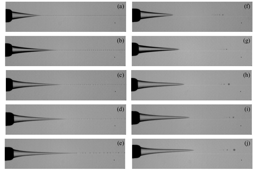
To illustrate the effect of the capillary number on the distribution of drop sizes, figure 1 as well as the three movies provided as supplementary material, show how water drops are generated and dispersed within co-flowing streams of different silicon oils with viscosities ranging from cp to cp at . Figures 1a-e reveal that, for each value of the viscosity ratio investigated, there exists a threshold outer velocity above which the thin liquid thread ejected from the tip of a conical drop breaks regularly, forming tiny droplets with very similar diameters. In the experimental situations depicted in figures 1f-j, the overall geometry of the drop attached at the injection tube is similar to that showed in figures 1a-e, but the jet issued at the apex of the cone is unsteady and breaks unevenly, forming droplets with a broad size distribution. It is interesting to note that the cone itself is steady even in cases in which the drop formation process is not periodic.
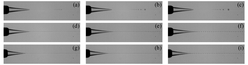
The reason for the differences observed in the two series of experiments depicted in figure 1 is that, in figures 1a-e , whereas in figures 1f-j, where is defined as the minimum value of the capillary number for which a train of uniform-sized drops is produced for fixed values of and . It is also interesting to note that, in contrast with the noticeable dependence of on deduced from the analysis of the type of experimental images depicted in figure 1, the results in figure 2 reveal that the critical capillary number is rather insensitive to changes in .
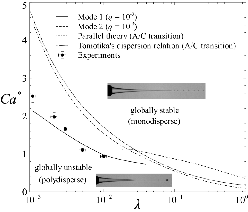
Since many different applications such as drug delivery demand that the size distribution of the drops composing the emulsion is as narrow as possible, it is desirable that the capillary number at which the coflow device is operated is larger than . It is thus our purpose in this paper to develop a theory to quantify and explain why drops with uniform sizes are produced only for values of the capillary number above the critical value deduced from the analysis of the experimental images in figures 1 and 2. Notice that, according to the experimental observations in figures 1 and 2, figure 3 shows that is a decreasing function of which does not appreciably vary with .
As a first attempt to predict and quantify the dependence of the critical capillary number on depicted in figure 3, let us recall that the non-regularity in the drop formation process is associated with the fact that the thin liquid thread from which drops are emitted, is itself unsteady. This experimental evidence suggests that the unstable capillary perturbations that give rise to the generation of drops cannot be convected downstream at a sufficiently large speed when . Therefore, the two regimes delimited by the experimental data points in figure 3 should correspond to those conditions for which unstable perturbations are either convected downstream the cone tip (convectively unstable flow), or are able to propagate upstream, thus inhibiting the formation of a steady jet (absolutely unstable flow).
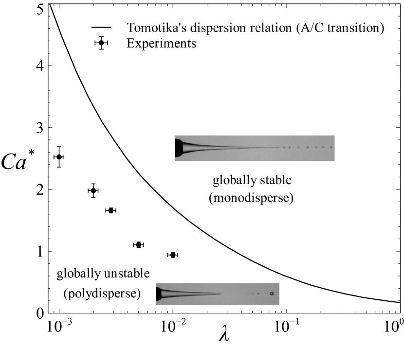
Previous studies (Sevilla et al., 2005; Utada et al., 2007, 2008; Guillot et al., 2007) have demonstrated that the experimentally observed transition from jetting to dripping in cylindrical capillary jets can be predicted by means of a local linear stability analysis of parallel streams (Huerre & Monkewitz, 1990). Thus, with the purpose of calculating the boundary separating the two different drop formation processes depicted in figures 1, 2 and in the movies provided as supplementary material, we have determined the values of the capillary number for which the temporal growth rate of the perturbations with zero group velocity is also equal to zero. The result obtained using Tomotika’s dispersion relation (Tomotika, 1935; Powers & Goldstein, 1997; Powers et al., 1998; Gañán Calvo, 2008), which describes the growth and propagation of perturbations in a cylindrical jet immersed into another immiscible liquid, is represented together with the experimental data in figure 3. Although the conditions of validity of Tomotika’s analysis are fulfilled at large distances from the injector, where the diameter of the liquid jet is nearly constant, figure 3 reveals that the parallel flow stability analysis predicts larger values for the critical capillary number than those measured experimentally. Consequently, the full jet, which strongly stretches in the downstream direction, is more stable than the cylindrical portion located far downstream.
To improve the agreement with experimental results, in this study we have performed a global stability analysis that takes into account the real shape of the stretched jet and describes the growth and propagation of perturbations without resorting to the parallel flow simplification used in previous studies (Tomotika, 1935; Gañán Calvo, 2008). To avoid the lengthy numerical computations associated with a global stability analysis in two or three spatial directions (see e.g. Zebib, 1987; Christodoulou & Scriven, 1992; Natarajan & Acrivos, 1993; Theofilis, 2011), in the present work we have developed a one-dimensional model based on slender-body theory that yields a single partial differential equation governing the spatiotemporal evolution of the jet radius. In Castro-Hernández et al. (2012) it was shown that the axial variations of both the steady shape of the jet and the outer flow field are very well reproduced by our previous theory. Here we will demonstrate that our global stability analysis, that resorts to a new equation for the jet radius, faithfully reproduces Tomotika’s dispersion relation in the long wave limit for the case of cylindrical jets of small viscosity ratio. Moreover, the experimentally measured values of the critical capillary number are very well reproduced since our final equation retains the axial dependence of the flow field in the formulation. Let us point out that the global stability analysis, developed in §2.2, shares many similarities with that by Rubio-Rubio, Sevilla & Gordillo (2013), where the global stability of gravitationally stretched jets is studied using a different one-dimensional model and excellent agreement with experiments is found.
2 Unsteady slender-body theory for the description of highly stretched jets in Stokes flow
One of the possible ways to analyze the conditions under which drops are formed regularly from the tip of the conical drop, would be to solve the unsteady velocity field using the integral formulation due to Ladyzhenskaya (1969), as was done in Castro-Hernández, Campo-Cortés & Gordillo (2012). However, following a strategy similar to that successfully applied to the case of liquid jets in air by García & Castellanos (1994); Eggers & Dupont (1994); Ambravaneswaran et al. (2004); Rubio-Rubio et al. (2013), the dynamics of the low Reynolds number jets depicted in figures 1-2 can be described using a much simpler one-dimensional approach which reveals the physics underlying the transition observed in these figures in a neat way. The central idea behind our one-dimensional theory can be understood by noticing that the slender jets shown in figures 1-2 resemble the case of drops immersed in a purely straining flow Stone (1994). The deformation of slender drops immersed in this type of flow field has been rigorously analyzed using asymptotic methods by Buckmaster (1971); Acrivos & Lo (1977) and, from these studies, it is learned that the outer flow field in the case of low viscous drops can be decomposed, in a first approximation, as the addition of the unperturbed flow field plus a distribution of sources located at the axis of symmetry. Since, in our case, the capillary that confines the outer fluid is ten times larger than the inner one, the dynamics of the jet is not affected by this confinement, as already demonstrated in Castro-Hernández et al. (2012). Therefore, the conclusions derived from Buckmaster (1971); Acrivos & Lo (1977) are fully applicable to the situation at hand, and figure 4 sketches the key idea under which our theory is built. This figure shows that the outer velocity field can be decomposed, in a first approximation, as the addition of two simpler flow fields: the unperturbed velocity field, which is the one that would exist in the coflowing device if the inner fluid was not injected (see figure 4a) and that induced on the outer stream by the presence of the jet (see 4b), which can be viewed as a perturbation to the former. From now on, , and will indicate time and the radial and axial coordinates respectively, with located at the exit of the injection tube, whereas will denote the radius of the jet. In our approach, the unperturbed velocity field is calculated numerically, by solving the Navier-Stokes equations in the zero Reynolds number limit (Stokes equations) subjected to the appropriate boundary conditions, as it will be explained below. Regarding the perturbed flow, we will take advantage of the fact that the outer velocity field induced by a slender jet of a low viscosity fluid immersed in an outer axisymmetric flow, as is the case of the experiments shown in figures 1 and 2, can be approximated to that created by a line of sources located at the axis of symmetry (Ashley & Landahl, 1965; Taylor, 1964; Buckmaster, 1971). The intensity of the source distribution, , must be such that the kinematic boundary condition is verified at the jet interface (see figure 4b).
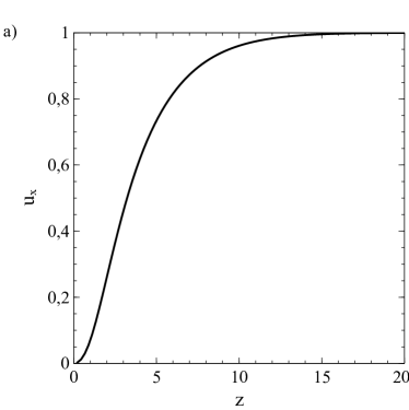
The representation of the outer flow field as the addition of two simpler velocity fields greatly facilitates the theoretical analysis of the spatiotemporal evolution of the jet. Firstly, notice that the numerical computation of the unperturbed flow field sketched in figure 4a is straightforward since this solution does not depend on , or : it is just a function of the geometry of the coflowing device and thus, it is unique for a given injector. But, what’s more, notice that the unperturbed velocity field does not even need to be known everywhere in the flow domain; instead, for our purposes, an accurate representation of the flow field in the vicinity of the axis of symmetry is enough. This is due to the fact that our interest here is to deduce an equation for , with for . Since the jet radius is located very near the axis of symmetry in most of the flow domain, all the information needed from the numerics to build our theoretical approach are just two functions: the axial component of the velocity at the axis, , as well as , where the subscript will be used in the following to denote quantities related to the unperturbed problem. Indeed, given these two functions, the analytical expression of the axial component of the unperturbed velocity field in the near-axis region will be expressed in Taylor series as . Moreover, the corresponding approximate expressions of both the radial component of the unperturbed velocity field namely, and of the unperturbed pressure field, , will be written in terms of and making use of the equations of continuity and momentum, as it will be shown below. Let us point out that the main difference between this work and those by Taylor (1964); Acrivos & Lo (1977); Hinch & Acrivos (1979); Sherwood (1983); Zhang (2004), where the deformation of drops and bubbles immersed in a purely straining flow in the limit of negligible inertial effects is studied, is that our theory retains the effect of the real outer flow field on the spatiotemporal evolution of the jet. More precisely, the effect of the injector geometry on the outer flow field will be represented in the equation to be deduced for through the two numerically determined functions and which, for the case of the specific geometry used in the experiments explained above, are represented graphically in figure 5 (see also Castro-Hernández et al. (2012)). Let us point out that the theory to be developed in §2.1 can be extended to any other types of axisymmetric geometries provided that the functions and are straightforwardly determined from the numerical solution of the Stokes equations subjected to the no slip boundary conditions imposed by the geometry of the injector and to the corresponding inflow/outflow boundary conditions.

2.1 Theory
The analysis presented in this section generalizes the work by Castro-Hernández et al. (2012), and aims to describe the propagation and growth of capillary disturbances in unsteady coflowing streams with negligible inertial effects. In our theory, the flow is represented as the superposition of the velocity field created by a distribution of sources with an unknown intensity plus the unperturbed flow field, which is the solution of the Stokes equations subjected to the the impermeability condition () that needs to be satisfied at: i) the tube exit, namely, the circle defined by , , ii) the outer surface of the injection tube, which is the cylinder of radius that extends along and iii) the inner surface of the outer tube, which is the cylinder of radius , where is defined in figure 4. Moreover, Poiseuille velocity profiles are imposed at the upstream and downstream boundaries of the flow domain (see Castro-Hernández et al. (2012) for further details). Regarding the perturbed flow, it was demonstrated by Taylor (1964); Acrivos & Lo (1977); Hinch & Acrivos (1979) that, when a slender drop or bubble with a viscosity much smaller than that of the outer fluid () is immersed within a straining flow, the first order modification to the unperturbed outer velocity field can be expressed as a superposition of sources located at the axis of symmetry. This is so because the contribution to the perturbed flow field associated with the addition of Stokeslets at , is of the order of (Buckmaster, 1971). Here, denotes the characteristic axial length scale for which the radius of the thread suffers variations of its same order of magnitude and, in the case of slender flows, . The same idea can thus be applied to describe the experiments depicted in figures 1-2 since, in all the cases under study here, and the resulting jet is slender, namely, . Therefore, the outer flow field can be approximately expressed as (Castro-Hernández et al., 2012),
| (1) |
In equation (1), and are the unit base vectors,
| (2) |
has been expressed as a function of making use of the continuity equation in cylindrical coordinates, namely, and, as it was pointed out above, the axial component of the velocity field is expressed retaining just the first two terms in the in Taylor series expansion of , what leads to
| (3) |
Moreover, in equation (1), only the radial component of the perturbed velocity field created by a distribution of sources, , has been retained in the analysis due to the fact that the order of magnitude of the corresponding axial component is (see, e.g. Ashley & Landahl (1965)).
Now notice that the unknown source intensity can be easily expressed as a function of the jet radius by means of the kinematic boundary condition at the interface,
| (4) |
Using the expression for given in equation (2), equation (4) yields
| (5) |
Making use of equation (5), the equation for can be easily deduced using the continuity equation
| (6) |
where it has been taken into account that the flow in the jet is the addition of the plug flow induced by the outer axial velocity field at the radial position where the interface is located plus the Poiseuille flow created by the inner pressure gradient, . It is of interest to point out that the flow within the jet in our one-dimensional theoretical approach may exhibit a recirculation bubble, in contrast with the type of one dimensional models which assume that the velocity profile within the jet is uniform (see, e.g. Ambravaneswaran et al. (2002, 2004); Rubio-Rubio et al. (2013) and references therein). Indeed, a recirculation bubble could exist in our case if the negative velocities of the parabolic velocity profile associated with an adverse inner pressure gradient (), were larger in magnitude than the corresponding positive velocity of the plug flow velocity profile.
In (6), notice that the inner stream pressure , which in the slender approximation is constant in the radial direction, is related to the outer pressure through the normal stress jump
| (7) |
where the term corresponding to the normal viscous stresses associated with the inner stream has been neglected due to the fact that . Moreover is the interfacial curvature, given by
| (8) |
with dots denoting derivatives with respect to . In equation (7), notice also that we have taken into account the fact that the velocity field created by the presence of the jet does not contribute to modify the outer pressure field. Indeed, the velocity field generated by a distribution of sources can be expressed in terms of the gradient of a velocity potential, namely, due to the fact that a single three dimensional source and thus, a superposition of sources, are solutions of the Laplace equation. Therefore, since in the zero Reynolds number limit the momentum equation reads
| (9) |
the only contribution to the outer pressure field comes from the unperturbed flow field, . Consequently, the outer axial pressure gradient in the near-axis region, where the jet surface is located, is calculated by means of the axial projection of the momentum equation,
| (10) |
where the expression for , given by equation (3), has been used. Taking , and as characteristic scales for length, time and pressure respectively, substituting (10) and (5) into the -derivative of (7), and introducing the final expression into (6), yields the following dimensionless partial differential equation for the jet radius,
| (11) |
with and in (11) given in figure 5. ¿From now on, lower case variables like those appearing in equation (11) indicate the dimensionless version of their dimensional counterparts and indicates the non dimensional expression for the interfacial curvature given by equation (8). Notice that the equation for the steady jet shape deduced in Castro-Hernández et al. (2012), namely
| (12) |
can be recovered by simply equating to zero the time derivatives in (11).
Let us point out that, in our description, the continuity of tangential stresses across the interface is never invoked since . In fact, this condition can be used to calculate the distribution of Stokeslets at the axis, what would introduce a higher order correction () to the velocity field created by the distribution of sources (Buckmaster, 1971). It is also interesting to note that, in our approach to deduce equation (11), terms of the order of have been neglected in the expression for the outer velocity field given by (1). However, the azimuthal curvature term , which is also of the order of , has been retained in equation (8). This apparent inconsistency is justified since, as pointed out in García & Castellanos (1994); Ambravaneswaran et al. (2002, 2004); Eggers & Villermaux (2008); Rubio-Rubio et al. (2013) and references therein, to improve the agreement with experiments in one dimensional models such as the one developed here, the exact expression of the interfacial curvature needs to be retained in the analysis of capillary dominated flows. Also, it can be appreciated in equation (10) that, in order for the contribution of to the inner pressure gradient to possess the same degree of accuracy as the contribution of the capillary pressure, the terms and , which are when compared to , have also been retained in the analysis.
2.2 Global stability analysis
To find whether the solutions of equation (12) are stable or not, we substitute the ansatz
| (13) |
into equation (11) and retain only linear terms in and its derivatives, yielding the following linear partial differential equation for the perturbed jet radius,
| (14) |
where the are five functions of and their -derivatives, whose expressions (35)-(39) are provided in Appendix A.
Equation (14) needs to be solved subjected to the boundary condition , and to the additional boundary condition expressing the fact that the flow rate at is independent of time and equal to , namely
| (15) |
Equation (15) has been deduced retaining only linear terms in and its derivatives in the expression resulting from the substitution of the ansatz (13) into equation (12).
Writing the perturbed radius as
| (16) |
the different eigenvalues and their corresponding global eigenfunctions are found numerically through a Chebychev spectral collocation method applied to the expression resulting from the substitution of the ansatz (16) into (14). For that purpose, the physical space , with the dimensionless jet length, is mapped into the Chebychev space through the transformation
| (17) |
To cluster as many points as possible in the cone-jet transition region, which is where the interfacial curvature suffers the strongest variations, the constant in (17) is chosen to be twice the distance from the injection nozzle where the curvature of the steady jet shape is minimum. Forcing the discrete version of equation (14) to be satisfied at the Chebychev collocation points within the physical domain (all the collocation points except those at the boundaries, namely and ) and imposing at the boundary condition as well as the one given by the discrete version of the equation resulting from the substitution of (16) into (15), yields the following linear system of equations for the eigenvalues and their corresponding eigenfunctions,
| (18) |
where the eigenvector contains the values of the perturbed jet radius at the collocation points. The matrices in equation (18) are respectively given by
| (19) |
and
| (20) |
where indicates the diagonal matrix whose elements are the values of the -dependent argument particularized at the collocation points, indicates the identity matrix, and the column vector
| (21) |
contains the value of the -th derivative of in the physical space at the collocation points. Let us point out that our stability results were independent of the numerical jet length, , provided that .
The steady solution , which is found solving the nonlinear equation (12) by means of a Newton-Raphson method, will be globally stable when the real parts of all the eigenvalues are negative, whereas it will be globally unstable if the real part of at least one eigenvalue, is positive. Thus, to find the function we proceed as follows: for given values of and , we first find the unperturbed jet shape by solving equation (12) for a sufficiently large value of Ca. The good agreement of the resulting function with experiments shown in Castro-Hernández et al. (2012), constitutes the first evidence that supports the accuracy of our generalized slender body theory. Once the steady solution is found, the matrices in equation (18) can be computed since they only depend on , its derivatives and on the control parameters . Then, we proceed to find the eigenvalues and their corresponding eigenvectors using standard Matlab functions (see figures 6 and 7). If the real parts of all eigenvalues are negative, as in the cases shown in figures 6a and 7a, Ca is decreased and the full process is repeated again until the real part of one of the eigenvalues crosses zero, as illustrated in figures 6d and 7d. Note that, for given values of and , the value of is determined by the condition that the real part of the leading eigenvalue is zero.
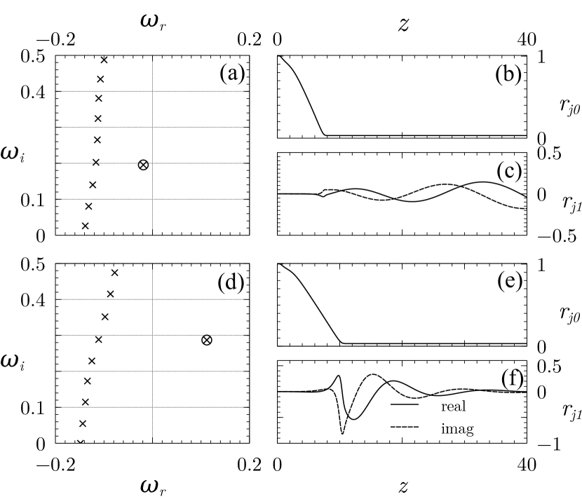
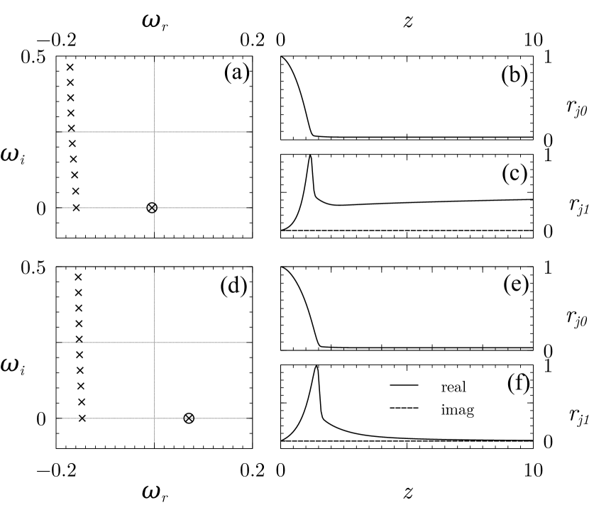
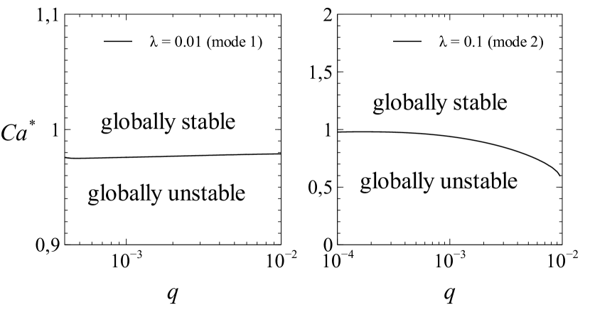
We have identified two different types of eigenfunctions that represent either a spatio-temporally oscillating mode (mode 1, see figure 6) or a non-oscillatory mode (mode 2, see figure 7). Both families are also differentiated by the fact that, contrarily to the case of the non-oscillatory mode, the amplitude of the oscillatory eigenfunction is virtually zero in the cone region, as it can be deduced from figure 6. At this point, let us anticipate that, within the ranges of and explored in this study, the stability analysis predicts that the oscillatory mode dominates over the steady one, so it is reasonable to expect that the shape of the eigenfunction depicted in figure 6f is somehow related with our experimental observations. This is indeed the case since, as revealed by figures 1 and 2, the cone region is unperturbed even in the cases in which the drop formation process is not periodic (see also the movies provided as supplementary material). Moreover, the maximum amplitude of the eigenfunction associated with the oscillatory mode is located slightly downstream the cone tip, and this is consistent with the experimental observation that the aperiodic formation process is associated with an unsteady emission of drops from a region located very close to the cone apex. Our global stability analysis also reveals that the value of the critical capillary number is hardly dependent on for values of the viscosity ratio (see figure 8). This finding is also in agreement with the experimental evidence shown in figure 2, where it can be appreciated that is rather insensitive to changes in . Therefore, in view of the slight variation of with shown in figure 8, the dependence of the critical capillary number with is calculated for a fixed value of . The result of this calculation, depicted in figure 9, compares favorably with experiments, a fact that further supports our theory. Since our theoretical predictions are much closer to the experimental observations than those obtained assuming that the jet is cylindrical, we can conclude that the strong variation of the jet radius in the axial direction plays an essential role in stabilizing the drop formation process.
We would like to emphasize that our analysis is able to predict the transition from the regular drop formation process that takes place when a thin steady ligament is issued from the cone apex (jetting regime) to the regime in which droplets detach aperiodically at the cone-jet region (dripping regime), but not the reverse dripping to jetting transition. Note also that the destabilization of the regular drop formation regime observed in our experiments shares some similarities with the transition from jetting to dripping observed in liquid jets stretched by gravity (Clanet & Lasheras, 1999; Ambravaneswaran et al., 2002, 2004), where the dripping regime manifests itself by the formation of drops right from or slightly downstream the exit of the injection tube. The main difference with the gravitational case is that, in the physical situation analyzed here, dripping occurs right from the tip of the conical drop, whose global shape is stable except very close to the microdrop emission region. The local oscillations appearing at the tip explain why the emission process is not periodic and leads to the formation of unevenly sized drops when the flow is globally unstable (see figures 1f-j, 6f and the movies provided as supplementary material). Let us point out that we also observe the formation of drops right from the exit tube, but this regime is found for values of the capillary number notably smaller than those investigated here (Suryo & Basaran, 2006). This type of dripping regime, which is much more similar to that observed in the gravitational case, has not been reported here since the diameters of the drops obtained are imposed by the geometry of the injector and, thus, are not of interest for applications due to the fact that their sizes are of the order of 100 microns or even larger.
2.3 Comparison with Tomotika’s stability analysis and elucidation of the physical mechanism leading to the higher stability exhibited by stretched jets
There is still a remaining question that needs to be answered: why do our stretched microjets exhibit a more stable behavior than their cylindrical counterparts? At first sight it could be thought that, since (see figure 5), the growth rate of perturbations decreases thanks to the kinematic mechanism described in Tomotika (1936) and in Frankel & Weihs (1985), whereby the amplitude of the perturbations decreases while their wavelenght increases due to the fact that fluid particles are elongated under the action of the outer straining flow field. However, we will show below that, although the jet is indeed stabilized thanks to this kinematic mechanism, the main reason for the higher stability exhibited by the stretched microjets of figures 1 and 2 is in fact related with the gradient of capillary pressure.
Indeed, let us adopt the slender approximation of assuming that the wavelength of the perturbation, , with the wavenumber, is much smaller than the length along which experiences variations of its same order of magnitude. This condition, clearly verified for , permits to look for traveling-wave solutions to equation (14), of the form , with and slowly varying functions of . At leading order, this approach provides the following dispersion relation for as a function of ,
| (22) |
where the term , provided in equation (27) of Appendix A, arises when linear perturbations in the expression for the full curvature of the jet are retained. Neglecting all the -derivatives of , what would correspond to the case of a purely cylindrical jet or to the solution of (12) at , leads to and to . The resulting dispersion relation (22) in the limit is identical to Tomotika’s long wave limit dispersion relation deduced by Powers & Goldstein (1997); Powers et al. (1998), a fact constituting a further proof of our theory. Applying the zero group velocity condition , to equation (22) in the limit , the boundary separating the absolutely and convectively unstable states can be calculated as explained in Huerre & Monkewitz (1990); Gordillo et al. (2001); Sevilla et al. (2005). The resulting A/C transition curve, shown in figure 9 (dash-dotted line), is very close to that obtained from the much more involved calculation (Powers & Goldstein, 1997; Powers et al., 1998; Gañán Calvo, 2008) that makes use of Tomotika’s dispersion relation (dotted line).
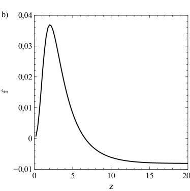
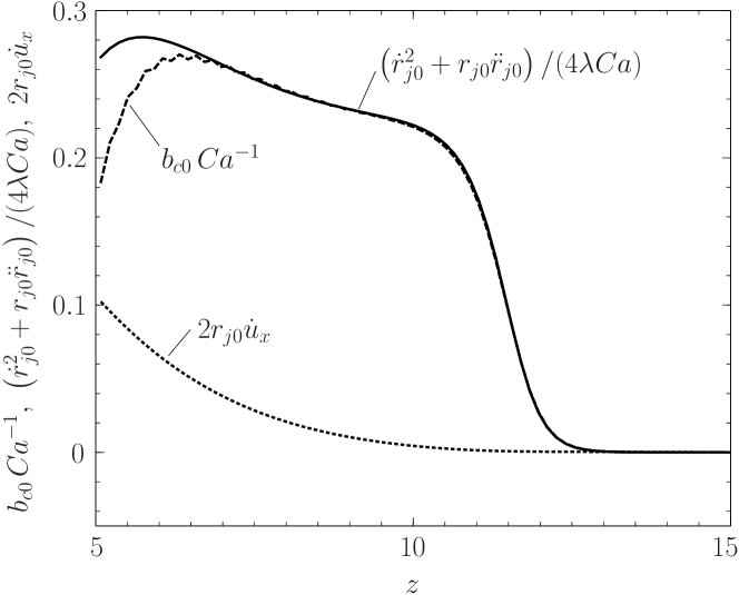
However, as stated above, to understand the higher stability of stretched jets we must retain the non-parallel terms in the dispersion relation (22) associated with axial variations of and . The main effect of non-parallel terms is to decrease the real part of , namely, the growth rate of perturbations. Indeed, since (see figure 5) and (see figure 10). It was already pointed out above that positive axial velocity gradients stabilize the jet (Tomotika, 1936; Frankel & Weihs, 1985; Eggers & Villermaux, 2008), but figure 10 reveals that near the tip of the conical drop, whose steady shape is depicted in figure 6b. The reason why the non-parallel term contributes to the stabilization of the stretched jet can be easily explained as follows: the gradients of capillary pressure in (6) produce an axial variation of the flow rate per unit length given by . Using the slender approximation for the curvature, namely, , linearizing the resulting expression around , and using dimensionless variables, yields which, as can be appreciated in figure 10, is an excellent approximation to in the cone-jet transition region. Therefore, since , perturbations such that (resp. ), that tend to increase (resp. decrease) the jet radius, cause (resp. ), leading to (resp. ) by virtue of the mass balance (6), thus explaining the stabilizing effect of the gradient of capillary pressure existing inside stretched jets.
3 Conclusions
In this paper we study the effect of the capillary number on the size distribution of the drops composing the microemulsions obtained when two immiscible liquid streams with co-flow at low Reynolds numbers and highly stretched liquid threads are produced (Suryo & Basaran, 2006; Marín et al., 2009). Our experiments reveal that, when and the flow rate ratio is such that , a liquid jet with a diameter substantially smaller than that of the injection tube is issued from the tip of a conical drop pinned at the exit of the injector. We find that this ligament is unsteady and breaks into unevenly sized droplets for with the critical capillary number and that, thanks to the fact that the growing capillary perturbations are convected downstream the cone-jet transition region, the thin liquid jet is steady and breaks into uniformly sized drops when . With the purpose of predicting the dependence of the critical capillary number on , we have first determined the values of Ca for which the group velocity of neutral waves is zero under the parallel flow assumption. The results of this analysis using the dispersion relation which describes the growth of capillary perturbations in cylindrical capillary jets (Tomotika, 1935), reveal that the boundary separating the absolutely unstable region from the convectively unstable one (Powers & Goldstein, 1997; Powers et al., 1998; Gañán Calvo, 2008) is well above the experimental values of the critical capillary number, a fact indicating that the non-cylindrical liquid ligaments of our experiments are more stable than their cylindrical counterparts. Thus, to improve the agreement between experiments and theory, we have performed a global stability analysis retaining the highly stretched shape of the liquid jet as well as realistic inner and outer velocity fields. For that purpose, following the slender body theory developed in Castro-Hernández et al. (2012), we have deduced the partial differential equation (11) that describes the spatiotemporal evolution of the jet radius and whose steady limit accurately reproduces the shape of the unperturbed liquid ligaments. Also, we have shown here that our equation (11) is able to reproduce Tomotika’s stability analysis in the limit of cylindrical jets of a low viscosity fluid, a fact that further supports the validity of our theory. Moreover, the results of our stability analysis, which are in fair agreement with experimental measurements, indicate that the regime in which monodisperse emulsions are produced corresponds to those values of the capillary number for which the cone-jet system is globally stable. We can thus conclude that the gradients of interfacial curvature and of axial velocity play an essential role in the propagation of perturbations along stretched capillary jets. Notice that this idea has also been successfully applied to describe the jetting to dripping transition experienced by gravitationally stretched capillary jets using the one-dimensional equations for the jet radius and the axial velocity (Rubio-Rubio et al., 2013). Let us point out that the simplicity of the one dimensional approximation used here to study the stability of stretched jets contrasts with the difficulty of analyzing the stability of two dimensional or three dimensional free surface flows (see e.g. Christodoulou & Scriven, 1992).
One of our major findings here is the discovery of a new stabilization mechanism that resorts to the existence of capillary pressure gradients inside low Reynolds number stretched jets that differs from the one based on the elongation of fluid particles (Tomotika, 1936). To conclude, we would like to emphasize that equation (11) is rather general in the sense that it can be applied to describe the propagation and growth of capillary perturbations along the jets produced, for instance, in flow-focusing devices operated at low Reynolds numbers. Indeed, notice that the influence of each particular geometry in the equation for the jet radius (11) comes through the functions and , which can be easily found numerically by solving Stokes equations subjected to the appropriate boundary conditions when the inner fluid is removed from the flow domain. Currently, we are extending the idea of decomposing the flow field as the addition of two simpler velocity fields to those cases in which the Reynolds number of the outer stream is large. The same type of ideas based on the slender body approach could also be applied to describe the stability of electrohydrodynamic tip streaming regimes that, under appropriate conditions, take place when electrical stresses act on the interface of liquid threads with a cone-jet structure (Fernandez de la Mora & Loscertales, 1994; Barrero & Loscertales, 2007; Collins et al., 2008, 2013).
Acknowledgements.
JMG and FCC thank financial support by the Spanish MINECO under Project DPI2011-28356-C03-01 and the Junta de Andalucía under Project P08-TEP-03997. AS thanks financial support by the Spanish MINECO under Project DPI2011-28356-C03-02. These research projects have been partly financed through European funds. The authors wish to express their gratitude to Elena de Castro-Henández for providing them with the numerical values of functions and and for her careful revision of the equations in the text.Appendix A
The partial differential equation (14) for the perturbed jet radius is the compact form of the following expression:
| (23) |
Notice that the five functions in equation (23) are deduced from the fact that
| (24) |
where
| (25) |
and
| (26) |
with .
Therefore,
| (27) |
| (28) |
| (29) |
| (30) |
and
| (31) |
Equation (23) admits solutions of the form leading, through the Chebychev discretization explained in the main text, to the following linear system of equations for the eigenvalues and their corresponding eigenfunctions,
| (32) |
with denoting a column vector containing the values of the perturbed radius at the collocation points,
| (33) |
and
| (34) |
with the five functions given by
| (35) |
| (36) |
| (37) |
| (38) |
and
| (39) |
References
- Acrivos & Lo (1977) Acrivos, A. & Lo, T. S. 1977 Deformation and breakup of a single slender drop in an extensional flow. J. Fluid Mech. 86, 641–672.
- Ambravaneswaran et al. (2004) Ambravaneswaran, B., Subramani, H. J., Phillips, S. D. & Basaran, O. A. 2004 Dripping-jetting transitions in a dripping faucet. Phys. Rev. Lett. 93, 034501(1–4).
- Ambravaneswaran et al. (2002) Ambravaneswaran, B., Wilkes, E. D. & Basaran, O. A. 2002 Drop formation from a capillary tube: Comparison of one-dimensional and two-dimensional analyses and occurrence of satellite drops. Phys. Fluids 14, 2606–2621.
- Anna et al. (2003) Anna, S. L., Bontoux, N. & Stone, H. A. 2003 Formation of dispersions using Flow Focusing in microchannels. Appl. Phys. Lett. 82, 364–366.
- Ashley & Landahl (1965) Ashley, H. & Landahl, M. 1965 Aerodynamics of wings and bodies. Adison-Wesley publishing company, inc., reading Mass. USA.
- Barrero & Loscertales (2007) Barrero, A. & Loscertales, I. G. 2007 Micro- and nanoparticles via capillary flows. Annu. Rev. Fluid Mech. 39, 89–106.
- Basaran (2002) Basaran, O. A. 2002 Small-scale free surface flows with breakup: drop formation and emerging applications. AIChE J. 48, 1842–1848.
- Buckmaster (1971) Buckmaster, J. D. 1971 Pointed bubbles in slow viscous flow. J. Fluid Mech. 55, 385–400.
- Gañán Calvo (2008) Gañán Calvo, A. M. 2008 Unconditional jetting. Phys. Rev. E 78, 026304.
- Castro-Hernández et al. (2012) Castro-Hernández, E., Campo-Cortés, F. & Gordillo, J. M. 2012 Slender-body theory for the generation of micrometre-sized emulsions through tip streaming. J. Fluid Mech. 698, 423–445.
- Christodoulou & Scriven (1992) Christodoulou, K. N. & Scriven, L. N. 1992 Discretization of free surface flows andd other moving boundary problems. J. Comp. Phys. 99 (4), 39–55.
- Clanet & Lasheras (1999) Clanet, C. & Lasheras, J. C. 1999 Transition from dripping to jetting. J. Fluid Mech. 383, 307–326.
- Collins et al. (2008) Collins, R. T., Jones, J. J., Harris, M. T. & Basaran, O. A. 2008 Electrohydrodynamic tip streaming and emission of charged drops from liquid cones. Nature Phys. 4 (4), 149–154.
- Collins et al. (2013) Collins, R. T., Sambath, K., Harris, M. T. & Basaran, O. A. 2013 Universal scaling laws for the didintegration of electrified drops. Proc. Acad. Sci. Amer. 110 (13), 4905–4910.
- Eggers & Dupont (1994) Eggers, J. & Dupont, T. 1994 Drop formation in a one-dimensional approximation of the navier-stokes equation. J. Fluid Mech. 262, 205–222.
- Eggers & Villermaux (2008) Eggers, J. & Villermaux, E. 2008 Physics of liquid jets. Rep. Prog. Phys. 71, 036601.
- Frankel & Weihs (1985) Frankel, I. & Weihs, D. 1985 Stability of a capillary jet with linearly increasing axial velocity (with application to shaped charges). J. Fluid Mech. 155, 289–307.
- García & Castellanos (1994) García, F. & Castellanos, A. 1994 One-dimensional models for slender axisymmetric viscous liquid jets. Phys. Fluids 6 (8), 2676–2689.
- Gordillo et al. (2001) Gordillo, J. M., Gañán Calvo, A. M. & Pérez-Saborid, M. 2001 Monodisperse microbubbling: Absolute instabilities in coflowing gas僕iquid jets. Phys. Fluids 13, 3839–3842.
- Guillot et al. (2007) Guillot, P., Colin, A., Utada, A. S. & Ajdari, A. 2007 Stability of a jet in confined pressure-driven biphasic flows at low Reynolds number. Phys. Rev. Lett. 99, 104502.
- Hinch & Acrivos (1979) Hinch, E. J. & Acrivos, A. 1979 Steady long slender droplets in two-dimensional straining motion. Jour. Fluid Mech. 91, 401–414.
- Huerre & Monkewitz (1990) Huerre, P. & Monkewitz, P. A. 1990 Local and global instabilities in spatially developing flows. Annu. Rev. Fluid Mech. 22, 473–537.
- Ladyzhenskaya (1969) Ladyzhenskaya, O. 1969 The Mathematical theory of viscous incompressible flows. Gordon & Breach, New York.
- Marín et al. (2009) Marín, A. G., Campo-Cortés, F. & Gordillo, J. M. 2009 Generation of micron-sized drops and bubbles through viscous coflows. Colloids Surf. A: Physicochem. Eng. Aspects 344, 2–7.
- Fernandez de la Mora & Loscertales (1994) Fernandez de la Mora, J. & Loscertales, I. 1994 The current emitted by highly conducting taylor cones. J. Fluid. Mech. 260, 155–184.
- Natarajan & Acrivos (1993) Natarajan, R. & Acrivos, A. 1993 The instability of the steady flow past spheres and disks. J. Fluid Mech. 254, 323–344.
- Powers et al. (1998) Powers, T., Zhang, D. F., Goldstein, R. E. & Stone, H. A. 1998 Propagation of a topological transition: The Rayleigh instability. Phys. Fluids 10, 1052–1057.
- Powers & Goldstein (1997) Powers, T. R. & Goldstein, R. E. 1997 Pearling and pinching: Propagation of Rayleigh instabilities. Phys. Rev. Lett. 78, 2555–2558.
- Rubio-Rubio et al. (2013) Rubio-Rubio, M., Sevilla, A. & Gordillo, J. 2013 On the thinnest steady threads obtained by gravitational stretching of capillary jets. J. Fluid Mech. 729, 471–483.
- Sevilla et al. (2005) Sevilla, A., Gordillo, J. M. & Martínez-Bazán, C. 2005 Transition from bubbling to jetting in a coaxial air-water jet. Phys. Fluids 17, 018105.
- Sherwood (1983) Sherwood, J. D. 1983 Tip streaming from slender drops in a nonlinear extensional flow. J. Fluid Mech. 144, 281–295.
- Stone (1994) Stone, H. A. 1994 Dynamics of drop deformation and breakup in viscous fluids. Annual Review of Fluid Mechanics 26, 65–102.
- Stone et al. (2004) Stone, H. A., Strook, A. D. & Adjari, A. 2004 Engineering flows in small devices: Microfluidics toward a lab-on-a-chip. Annu. Rev. Fluid Mech. 36, 381–411.
- Suryo & Basaran (2006) Suryo, R. & Basaran, O. A. 2006 Tip streaming from a liquid drop forming from a tube in a co-flowing outer fluid. Phys. Fluids 18, 082102.
- Taylor (1964) Taylor, G. I. 1964 Conical free surfaces and fluid interfaces. Proceedings of the 11th International Congress of Applied Mechanics (Munich) pp. 790–796.
- Theofilis (2011) Theofilis, V. 2011 Global linear instability. Annu. Rev. Fluid Mech. 43, 319–352.
- Tomotika (1935) Tomotika, S. 1935 On the instability of a cylindrical thread of a viscous liquid surrounded by another viscous fluid. Proc. Roy. Soc. 150, 322–337.
- Tomotika (1936) Tomotika, S. 1936 Breaking up of a drop of viscous liquid immersed in another viscous fluid which is extending at a uniform rate. Proc. Roy. Soc. 153, 302–318.
- Utada et al. (2008) Utada, A. S., Fernández-Nieves, A., Gordillo, J. M. & Weitz, D. 2008 Absolute instability of a liquid jet in a coflowing stream. Phys. Rev. Lett. 100, 014502.
- Utada et al. (2007) Utada, A. S., Fernández-Nieves, A., Stone, H. A. & Weitz, D. 2007 Dripping to jetting transitions in co-flowing liquid streams. Phys. Rev. Lett. 99, 094502.
- Zebib (1987) Zebib, A. 1987 Stability of viscous flow past a circular cylinder. J. Engng. Math. 21, 155–165.
- Zhang (2004) Zhang, W. W. 2004 Viscous entrainment from a nozzle: singular liquid spouts. Phys. Rev. Lett. 93, 184502.