Equilibration and prethermalization in the Bose-Hubbard and Fermi-Hubbard models

Abstract

We study the Bose and Fermi Hubbard model in the (formal) limit of large coordination numbers $Z\gg 1$. Via an expansion into powers of $1/Z$, we establish a hierarchy of correlations which facilitates an approximate analytical derivation of the time-evolution of the reduced density matrices for one and two sites etc. With this method, we study the quantum dynamics (starting in the ground state) after a quantum quench, i.e., after suddenly switching the tunneling rate $J$ from zero to a finite value, which is still in the Mott regime. We find that the reduced density matrices approach a (quasi) equilibrium state after some time. For one lattice site, this state can be described by a thermal state (within the accuracy of our approximation). However, the (quasi) equilibrium state of the reduced density matrices for two sites including the correlations cannot be described by a thermal state. Thus, real thermalization (if it occurs) should take much longer time. This behavior has already been observed in other scenarios and is sometimes called “pre-thermalization.” Finally, we compare our results to numerical simulations for finite lattices in one and two dimensions and find qualitative agreement.

I Introduction

Despite decades of research, our understanding of the quantum dynamics of interacting many-particle systems is still far from complete. One of the major unsolved questions (or rather a set of questions) is the problem of thermalization of isolated quantum systems D91 ; S94 ; BBS03 ; BBW04 ; CC06 ; CC07 ; RDYO07 ; RDO08 ; EHKKMWW09 ; MK09 ; CR10 ; PSSV11 ; KWE11 ; GME11 ; KISD11 ; BCH11 ; RS12 ; R13 . In one version, this question can be posed in the following way: Given an interacting quantum many-body system on an infinite lattice in a globally excited state, do all observables involving a finite number of lattice sites settle down to a value which is consistent with a thermal state described by a suitable temperature? Note that we do not consider thermalization induced by the coupling to some large thermal reservoir, but the intrinsic mechanism occurring in closed quantum systems during unitary evolution.

The global nature of the excitation is necessary because a local excitation (with a finite total energy) would typically disperse to infinity and leave the system locally at its ground state after some time. One option to create such a global excitation is a quantum quench: Starting in the ground state of a given Hamiltonian, one suddenly (or at least non-adiabatically) changes some of the parameters, e.g., the external magnetic field or a coupling strength, and thus induces a global departure from the ground state (of the modified Hamiltonian).

This behavior crucially depends on the structure of the Hamiltonian. Integrable models, for example, possess an infinite set of non-trivial conserved quantities. If these conserved quantities are measurable with local observables, there is no real thermalization. Instead, one should describe the state by a generalized Gibbs ensemble which contains a Lagrange multiplier for each conserved quantity. This motivates the study of non-integrable models, such as the Bose-Hubbard model and Fermi-Hubbard model in more than one dimension considered here. The models are prototypical examples for simple and yet non-trivial lattice Hamiltonians and can also be realized experimentally, for example, with ultra-cold atoms in optical lattices JZ07 ; MO06 ; LSADSS07 ; BDZ08 ; Y09 ; LSA12 .

Even if the thermalization occurs, there is still the question of the time scales involved, for example: How fast does the system thermalize and do some observable thermalize faster than others? Are there intermediate stages and how fast do the quantum correlations spread? The last question is related to the others since the unitary evolution of a closed quantum system implies that an initially pure state will remain pure. Hence the description of a local state by a thermal (i.e., mixed) density matrix is only possible due to quantum correlations with some remote part of the lattice which is averaged over.

Quantum quenches have been considered before, for bosons and for fermions. For bosons, many studies have been devoted to one spatial dimension by employing exact diagonalization KLA07 ; BKLO08 ; GR09 ; GR10 , time-dependent density matrix renormalization group theory (t-DMRG) KLA07 ; CDEO08 ; CFMSE08 ; FCMSE08 ; LK08 ; BRK11 ; BPBRK12 , and Jordan-Wigner fermionization BPCK12 . For corresponding experiments, see Refs. GMHB02 ; KWS06 ; ST12 ; CBPE12 ; GKLKRSMADS12 . However, thermalization in one spatial dimension is quite different from the behavior in higher dimensions because quasi-particles in one dimension cannot thermalize via elastic two-body collisions due to energy-momentum conversation.

For bosons in higher dimensions, many of the methods which work well in one dimension cannot be applied. Apart from some general statements concerning the relaxation of a quantum system towards equilibrium CDEO08 ; CFMSE08 ; FCMSE08 , quantum quenches have been studied by using certain approximations, such as Bogoliubov-type approximations or strong-coupling perturbation theory SUXF06 ; FSU08 ; NM13a ; NM13b , the Gutzwiller approximation NHM11 , or related (semi) classical methods SB08 ; SB10 ; SWD12 , as well as (truncated) exact diagonalization KLA07 . However, these approximations are only reliable in certain regions of parameter space. For an experimental realization of the quench from the Mott-insulator to the superfluid regime, see Ref. CWBD11 .

For fermions in one spatial dimension, the integrability of the Fermi-Hubbard model facilitates the derivation of the exact evolution after a quench including effects such as “pre-thermalization” KE08 ; KWE11 ; HU13 . Again, in higher dimensions, appropriate approximations are necessary, such as a time-dependent Monte-Carlo method GA12 , time-dependent dynamical mean field theory EKW09 ; EKW10 ; A10 ; A11 ; WTE12 , the Gutzwiller ansatz for fermions SF10 ; SF11 ; SSF12 , the flow equation method MK08 ; MK09 ; MK10 ; EHKKMWW09 , or effective quasi-particle methods SGJ10 .

In the present work, we study the quantum evolution after a quench in the Bose and Fermi Hubbard models. We develop and employ an analytic approximation technique which is controlled by an expansion into powers of the inverse coordination number $1/Z$ (see also HSH09 ). Note that the $1/Z$-expansion employed here is somewhat similar to time-dependent dynamical mean field theory (t-DMFT), but the $1/\sqrt{Z}$ scaling of the hopping term in the Hamiltonian (used in t-DMFT) is replaced by a $1/Z$ scaling in our approach – which allows us to derive analytic expressions for the time-dependent correlation functions after the quench.

II Bose-Hubbard Model

The Bose-Hubbard model is one of the most simple and yet non-trivial models in condensed matter theory FWGF89 ; J98 ; Z03 . It describes identical bosons hopping on a lattice with the tunneling rate $J$. In addition, two (or more) bosons at the same lattice site repel each other with the interaction energy $U$. The Hamiltonian reads

$$\hat{H}=-\frac{J}{Z}\sum_{\mu\nu}T_{\mu\nu}\hat{b}^{\dagger}_{\mu}\hat{b}_{\nu}+\frac{U}{2}\sum_{\mu}\hat{n}_{\mu}(\hat{n}_{\mu}-1)\,.$$ (1)

Here $\hat{b}^{\dagger}_{\mu}$ and $\hat{b}_{\nu}$ are the creation and annihilation operators at the lattice sites $\mu$ and $\nu$, respectively, which obey the usual commutation relations

$$\left[\hat{b}_{\nu},\hat{b}_{\mu}^{\dagger}\right]=\delta_{\mu\nu}\;,\,\left[\hat{b}_{\nu}^{\dagger},\hat{b}_{\mu}^{\dagger}\right]=\left[\hat{b}_{\nu},\hat{b}_{\mu}\right]=0\,.$$ (2)

The lattice structure is encoded in the adjacency matrix $T_{\mu\nu}$ which equals unity if $\mu$ and $\nu$ are tunneling neighbors (i.e., if a particle can hop from $\mu$ to $\nu$) and zero otherwise. The number of tunneling neighbors at a given site $\mu$ yields the coordination number $Z=\sum_{\nu}T_{\mu\nu}$ (we assume a translationally invariant lattice). Finally, $\hat{n}_{\mu}=\hat{b}^{\dagger}_{\mu}\hat{b}_{\mu}$ is the number operator and we assume unit filling $\langle\hat{n}_{\mu}\rangle=1$ in the following. Note that the total particle number $\hat{N}=\sum_{\mu}\hat{n}_{\mu}$ is conserved $[\hat{H},\hat{N}]=0$.

The Bose-Hubbard model is considered as one of the prototypical examples for a quantum phase transition sachdev . If the interaction term dominates $U\gg J$, the bosons are pinned to their lattice sites and we have the Mott insulator state

$$\left|\Psi_{\rm Mott}^{J=0}\right>=\bigotimes\limits_{\mu}\left|1\right>_{\mu}=\prod\limits_{\mu}\hat{b}_{\mu}^{\dagger}\left|0\right>\;\leadsto\;\hat{H}\left|\Psi_{\rm Mott}^{J=0}\right>=0\,,$$ (3)

which is fully localized. If the hopping rate dominates $U\ll J$, on the other hand, the particles can propagate freely across the lattice and become completely delocalized

$$\left|\Psi_{\rm superfluid}^{U=0}\right> = \frac{1}{\sqrt{N!N^{N}}}\left(\sum_{\mu}\hat{b}_{\mu}^{\dagger}\right)^{N}\left|0\right>$$ (4)

$$= \frac{1}{\sqrt{N!}}\left(\hat{b}_{\mbox{\boldmath$\scriptstyle k$}=0}^{\dagger}\right)^{N}\left|0\right>\,,$$

which is the superfluid phase. Obviously, the Mott state (3) does not have any correlations footnote-correlations between lattice sites, for example $\langle\hat{b}^{\dagger}_{\mu}\hat{b}_{\nu}\rangle_{\rm Mott}=\delta_{\mu\nu}$, whereas the superfluid state in (4) shows correlations across the whole lattice $\langle\hat{b}^{\dagger}_{\mu}\hat{b}_{\nu}\rangle_{\rm superfluid}=1$. Furthermore, the Mott insulator state is separated by a finite energy gap from the lowest excited state, while the superfluid state possesses sound-like modes with arbitrarily low energies (for an infinitely large lattice $N\to\infty$). Finally, the Bose-Hubbard model can be realized experimentally (to a very good approximation) with ultra-cold atoms in optical lattices B05 ; S07 ; RSN97 and it was even possible to observe the aforementioned phase transition in these systems G02 .

In spite of its simplicity, the Bose-Hubbard model (1) cannot be solved analytically. Numerical simulations are limited to reduced sub-spaces or small systems sizes, see Section IX below. Analytical approaches are based on suitable approximations. In order to control the error of these approximations, they should be based on an expansion in term of some large or small control parameter. For the Bose-Hubbard model (1), one could consider the limit of large $\langle\hat{n}_{\mu}\rangle\gg 1$ or small $\langle\hat{n}_{\mu}\rangle\ll 1$ filling SUXF06 ; FSU08 , for example, or the limit of weak coupling $U\ll J$ or strong coupling $U\gg J$ FM94 ; FM96 ; DZ06 ; FKKKT2009 . However, none of these limits is particularly well suited for studying the Mott–superfluid phase transition. To this end, we consider the limit $Z\gg 1$ in the following and employ an expansion into powers of $1/Z$ as small control parameter. Note that an expansion in powers of $1/Z$ was also used to derive bosonic dynamical mean-field equations (which were then solved numerically) in HSH09 ; LBHH11 ; LBHH12 .

III Hierarchy of Correlations

Let us consider general Hamiltonians of the form

$$\hat{H}=\frac{1}{Z}\sum_{\mu\nu}\hat{H}_{\mu\nu}+\sum_{\mu}\hat{H}_{\mu}\,,$$ (5)

which includes the bosonic and fermionic Hubbard models (1) and (57) as special cases. The quantum evolution of the density operator $\hat{\rho}$ describing the state of the full lattice can be written as

$$i\partial_{t}\hat{\rho}=\left[\hat{H},\hat{\rho}\right] = \frac{1}{Z}\sum_{\mu\nu}\left[\hat{H}_{\mu\nu},\hat{\rho}\right]+\sum_{\mu}\left[\hat{H}_{\mu},\hat{\rho}\right]$$ (6)

$$= \frac{1}{Z}\sum_{\mu\nu}\,\widehat{\cal L}_{\mu\nu}\hat{\rho}+\sum_{\mu}\,\widehat{\cal L}_{\mu}\hat{\rho}\,,$$

where we have introduced the Liouville super-operators $\,\widehat{\cal L}_{\mu\nu}$ and $\,\widehat{\cal L}_{\mu}$ as short-hand notation. As the next step, we introduce the reduced density matrices for one or more lattice sites via averaging (tracing) over all other sites

$$\hat{\rho}_{\mu} = \,{\rm Tr}_{\not\mu}\{\hat{\rho}\}\;,\quad\hat{\rho}_{\mu\nu}=\,{\rm Tr}_{\not\mu\not\nu}\{\hat{\rho}\}\,,$$ (7)

and so on. Note that $\,{\rm Tr}\{\hat{\rho}\}=1$ implies $\,{\rm Tr}_{\mu}\{\hat{\rho}_{\mu}\}=1$ and $\,{\rm Tr}_{\mu\nu}\{\hat{\rho}_{\mu\nu}\}=1$ etc. Next we define correlated parts of the reduced density matrices via

$$\hat{\rho}_{\mu\nu} = \hat{\rho}_{\mu\nu}^{\rm corr}+\hat{\rho}_{\mu}\hat{\rho}_{\nu}$$ (8)

$$\hat{\rho}_{\mu\nu\lambda} = \hat{\rho}_{\mu\nu\lambda}^{\rm corr}+\hat{\rho}_{\mu\nu}^{\rm corr}\hat{\rho}_{\lambda}+\hat{\rho}_{\mu\lambda}^{\rm corr}\hat{\rho}_{\nu}+\hat{\rho}_{\nu\lambda}^{\rm corr}\hat{\rho}_{\mu}+\hat{\rho}_{\mu}\hat{\rho}_{\nu}\hat{\rho}_{\lambda}\,,$$

and analogously for more lattice sites. As a consequence, we obtain from Eq. (6) the evolution equation for the one-point density matrix

$$i\partial_{t}\hat{\rho}_{\mu}=\frac{1}{Z}\sum_{\kappa\neq\mu}\,{\rm Tr}_{\kappa}\left\{\,\widehat{\cal L}^{S}_{\mu\kappa}(\hat{\rho}^{\rm corr}_{\mu\kappa}+\hat{\rho}_{\mu}\hat{\rho}_{\kappa})\right\}+\,\widehat{\cal L}_{\mu}\hat{\rho}_{\mu}\,,$$ (9)

where $\,\widehat{\cal L}_{\mu\nu}^{S}=\,\widehat{\cal L}_{\mu\nu}+\,\widehat{\cal L}_{\nu\mu}$ denotes the symmetrized form. Obviously, solving this equation exactly requires knowledge of the two-point correlation $\hat{\rho}^{\rm corr}_{\mu\kappa}$. The time-evolution of this quantity can also be obtained from Eq. (6) and reads

$$i\partial_{t}\hat{\rho}^{\rm corr}_{\mu\nu} = \,\widehat{\cal L}_{\mu}\hat{\rho}^{\rm corr}_{\mu\nu}+\frac{1}{Z}\,\widehat{\cal L}_{\mu\nu}(\hat{\rho}^{\rm corr}_{\mu\nu}+\hat{\rho}_{\mu}\hat{\rho}_{\nu})$$ (10)

$$-\frac{\hat{\rho}_{\mu}}{Z}\,{\rm Tr}_{\mu}\left\{\,\widehat{\cal L}^{S}_{\mu\nu}(\hat{\rho}^{\rm corr}_{\mu\nu}+\hat{\rho}_{\mu}\hat{\rho}_{\nu})\right\}$$

$$+\frac{1}{Z}\sum_{\kappa\not=\mu,\nu}\,{\rm Tr}_{\kappa}\left\{\,\widehat{\cal L}^{S}_{\mu\kappa}(\hat{\rho}^{\rm corr}_{\mu\nu\kappa}+\hat{\rho}^{\rm corr}_{\mu\nu}\hat{\rho}_{\kappa}+\hat{\rho}^{\rm corr}_{\nu\kappa}\hat{\rho}_{\mu})\right\}$$

$$+(\mu\leftrightarrow\nu)\,.$$

As one would expect, this equation contains the three-point correlator $\hat{\rho}^{\rm corr}_{\mu\nu\kappa}$, and similarly the evolution equation for $\hat{\rho}^{\rm corr}_{\mu\nu\kappa}$ contains the four-point correlator etc. In general, one cannot exactly solve this infinite set of equations. However, the limit $Z\gg 1$ facilitates an approximate solution that can be systematically improved.

Let us start from an initial state $\hat{\rho}^{\rm in}=\bigotimes_{\mu}\hat{\rho}^{\rm in}_{\mu}$ that does not have any correlations (i.e., $\hat{\rho}^{\rm corr}_{\mu\nu}(0)=0$ and $\hat{\rho}^{\rm corr}_{\mu\nu\kappa}(0)=0$, etc.) such as the Mott state (3). In this case, the right-hand side of Eq. (10) scales as $1/Z$ and thus the time evolution creates only small correlations $\hat{\rho}^{\rm corr}_{\mu\nu}(t)$. If these correlations are small initially, $\hat{\rho}^{\rm corr}_{\mu\nu}(0)=\,{\cal O}(1/Z)$, they remain small at least for a finite time. The order of terms in the second line of Eq. (10) is determined by the correlated parts of the density matrices. This is because the summation over $\kappa$ gives at most a factor of $Z$ which is compensated by the factor $1/Z$ in front of the sum. In addition, we can neglect the term in Eq. (9) which contains $\hat{\rho}^{\rm corr}_{\mu\nu}$ because it is of the higher order than the others. Thus, we arrive at an approximate equation containing one-point density matrices only

$$i\partial_{t}\hat{\rho}_{\mu}=\frac{1}{Z}\sum_{\kappa\neq\mu}\,{\rm Tr}_{\kappa}\left\{\,\widehat{\cal L}^{S}_{\mu\kappa}\hat{\rho}_{\mu}\hat{\rho}_{\kappa}\right\}+\,\widehat{\cal L}_{\mu}\hat{\rho}_{\mu}+\,{\cal O}(1/Z)\;.$$ (11)

The approximate solution $\hat{\rho}_{\mu}^{0}$ of this self-consistent equation is valid to lowest order in $1/Z$, i.e., $\hat{\rho}_{\mu}=\hat{\rho}_{\mu}^{0}+\,{\cal O}(1/Z)$ and reproduces the well-known Gutzwiller ansatz G63 ; RK91 ; J98 . If we now insert this approximate solution $\hat{\rho}_{\mu}^{0}$ into Eq. (10), we get an approximate evolution equation for the two-point correlator

$$i\partial_{t}\hat{\rho}^{\rm corr}_{\mu\nu} = \,\widehat{\cal L}_{\mu}\hat{\rho}^{\rm corr}_{\mu\nu}+\frac{1}{Z}\,\widehat{\cal L}_{\mu\nu}\hat{\rho}^{0}_{\mu}\hat{\rho}^{0}_{\nu}-\frac{\hat{\rho}^{0}_{\mu}}{Z}\,{\rm Tr}_{\mu}\left\{\,\widehat{\cal L}^{S}_{\mu\nu}\hat{\rho}^{0}_{\mu}\hat{\rho}^{0}_{\nu}\right\}$$ (12)

$$+\frac{1}{Z}\sum_{\kappa\not=\mu,\nu}\,{\rm Tr}_{\kappa}\left\{\,\widehat{\cal L}^{S}_{\mu\kappa}(\hat{\rho}^{\rm corr}_{\mu\nu}\hat{\rho}^{0}_{\kappa}+\hat{\rho}^{\rm corr}_{\nu\kappa}\hat{\rho}^{0}_{\mu})\right\}$$

$$+(\mu\leftrightarrow\nu)+\,{\cal O}(1/Z^{2})\,.$$

Since we assumed that the three-point correlations $\hat{\rho}^{\rm corr}_{\mu\nu\kappa}$ are suppressed by $\,{\cal O}(1/Z^{2})$, they do not spoil this line of arguments. In complete analogy, it is possible to derive the evolution equations for any $\ell$-point function, see Appendix A. Thus, we find that $\ell$-point correlations are suppressed as $\,{\cal O}(1/Z^{\ell-1})$, i.e.,

$$\hat{\rho}_{\mu} = \,{\cal O}\left(Z^{0}\right)\;,\quad\hat{\rho}^{\rm corr}_{\mu\nu}=\,{\cal O}\left(1/Z\right)\;,$$

$$\hat{\rho}^{\rm corr}_{\mu\nu\kappa} = \,{\cal O}\left(1/Z^{2}\right)\;,\quad\hat{\rho}^{\rm corr}_{\mu\nu\kappa\lambda}=\,{\cal O}\left(1/Z^{3}\right)\;,$$ (13)

and so on, see Appendix A. The hierarchy (III) is related to the quantum de Finetti theorem CKMR07 , the generalized cumulant expansion K62 , and the Bogoliubov-Born-Green-Kirkwood-Yvon (BBGKY) hierarchy B75 , but we are considering lattice sites instead of particles. As an example for the four-point correlator, let us consider observables $\hat{A}_{\mu}$, $\hat{B}_{\nu}$, $\hat{C}_{\kappa}$, and $\hat{D}_{\lambda}$ at four different lattice sites, which have vanishing on-site expectation values $\langle\hat{A}_{\mu}\rangle=\langle\hat{B}_{\nu}\rangle=\langle\hat{C}_{\kappa}\rangle=\langle\hat{D}_{\lambda}\rangle=0$. In this case, the hierarchy (III) implies

$$\langle\hat{A}_{\mu}\hat{B}_{\nu}\hat{C}_{\kappa}\hat{D}_{\lambda}\rangle = \langle\hat{A}_{\mu}\hat{B}_{\nu}\rangle\langle\hat{C}_{\kappa}\hat{D}_{\lambda}\rangle+\langle\hat{A}_{\mu}\hat{C}_{\kappa}\rangle\langle\hat{B}_{\nu}\hat{D}_{\lambda}\rangle$$ (14)

$$+\langle\hat{A}_{\mu}\hat{D}_{\lambda}\rangle\langle\hat{B}_{\nu}\hat{C}_{\kappa}\rangle+\,{\cal O}\left(1/Z^{3}\right)\,,$$

which resembles the Wick theorem in free quantum field theory (even though the quantum system considered here is strongly interacting).

IV Mott Insulator State

Now let us apply the hierarchy discussed above to the Bose-Hubbard model (1). To this end, we start with the factorizing Mott state (3) at zero hopping rate $J=0$ as our initial state

$$\hat{\rho}^{\rm in}=\bigotimes\limits_{\mu}\hat{\rho}^{\rm in}_{\mu}=\bigotimes\limits_{\mu}\left|1\right>_{\mu}\!\left<1\right|\,.$$ (15)

Then we slowly switch on the hopping rate $J(t)$ until we reach its final value. In view of the finite energy gap, the adiabatic theorem implies that we stay very close to the real ground state of the system if we do this slowly enough. Of course, we cannot cross the phase transition in this way (i.e., adiabatically) since the energy gap vanishes at the critical point, see Section V below.

Since we have $\langle\hat{b}_{\mu}\rangle=0$ in the Mott state, Eq. (11) simplifies to

$$i\partial_{t}\hat{\rho}_{\mu} \approx \frac{1}{Z}\sum_{\kappa\neq\mu}\,{\rm Tr}_{\kappa}\left\{\,\widehat{\cal L}^{S}_{\mu\kappa}\hat{\rho}_{\mu}\hat{\rho}_{\kappa}\right\}+\,\widehat{\cal L}_{\mu}\hat{\rho}_{\mu}=0$$ (16)

$$\leadsto\,\hat{\rho}_{\mu}^{0}=\left|1\right>_{\mu}\!\left<1\right|\,.$$

Thus, to zeroth order in $1/Z$ (i.e., on the Gutzwiller mean-field level), the Mott insulator state $\hat{\rho}_{\mu}^{0}$ for finite $J$ has the same form as for $J=0$. To obtain the first order in $1/Z$, we insert this result into (12). Again using $\langle\hat{b}_{\mu}\rangle=0$, we find

$$i\partial_{t}\hat{\rho}^{\rm corr}_{\mu\nu} = \left(\,\widehat{\cal L}_{\mu}+\,\widehat{\cal L}_{\nu}\right)\hat{\rho}^{\rm corr}_{\mu\nu}+\frac{1}{Z}\,\widehat{\cal L}_{\mu\nu}^{S}\hat{\rho}_{\mu}^{0}\hat{\rho}_{\nu}^{0}$$ (17)

$$+\frac{1}{Z}\sum_{\kappa\not=\mu,\nu}\,{\rm Tr}_{\kappa}\left\{\,\widehat{\cal L}^{S}_{\mu\kappa}\hat{\rho}^{\rm corr}_{\nu\kappa}\hat{\rho}_{\mu}^{0}+\,\widehat{\cal L}^{S}_{\nu\kappa}\hat{\rho}^{\rm corr}_{\mu\kappa}\hat{\rho}_{\nu}^{0}\right\}$$

$$+\,{\cal O}(1/Z^{2})\,.$$

Formally, this is an evolution equation for an infinite dimensional matrix $\hat{\rho}^{\rm corr}_{\mu\nu}$. Fortunately, however, it suffices to consider a few elements only. If we introduce $\hat{p}_{\mu}=\left|1\right>_{\mu}\!\left<2\right|$ and $\hat{h}_{\mu}=\left|0\right>_{\mu}\!\left<1\right|$ as local particle and hole operators (these excitations are sometimes KJSW90 ; CBPE12 ; BPCK12 called doublons and holons), all the interesting physics can be captured by their correlation functions (for $\mu\neq\nu$)

$$f_{\mu\nu}^{11} = \langle\hat{h}^{\dagger}_{\mu}\hat{h}_{\nu}\rangle=\,{\rm Tr}\left\{\hat{\rho}\,\hat{h}^{\dagger}_{\mu}\hat{h}_{\nu}\right\}=\,{\rm Tr}_{\mu\nu}\left\{\hat{\rho}^{\rm corr}_{\mu\nu}\hat{h}^{\dagger}_{\mu}\hat{h}_{\nu}\right\}\,,$$

$$f_{\mu\nu}^{12} = \langle\hat{h}^{\dagger}_{\mu}\hat{p}_{\nu}\rangle=\,{\rm Tr}\left\{\hat{\rho}\,\hat{h}^{\dagger}_{\mu}\hat{p}_{\nu}\right\}=\,{\rm Tr}_{\mu\nu}\left\{\hat{\rho}^{\rm corr}_{\mu\nu}\hat{h}^{\dagger}_{\mu}\hat{p}_{\nu}\right\}\,,$$

$$f_{\mu\nu}^{21} = \langle\hat{p}^{\dagger}_{\mu}\hat{h}_{\nu}\rangle=\,{\rm Tr}\left\{\hat{\rho}\,\hat{p}^{\dagger}_{\mu}\hat{h}_{\nu}\right\}=\,{\rm Tr}_{\mu\nu}\left\{\hat{\rho}^{\rm corr}_{\mu\nu}\hat{p}^{\dagger}_{\mu}\hat{h}_{\nu}\right\}\,,$$

$$f_{\mu\nu}^{22} = \langle\hat{p}^{\dagger}_{\mu}\hat{p}_{\nu}\rangle=\,{\rm Tr}\left\{\hat{\rho}\,\hat{p}^{\dagger}_{\mu}\hat{p}_{\nu}\right\}=\,{\rm Tr}_{\mu\nu}\left\{\hat{\rho}^{\rm corr}_{\mu\nu}\hat{p}^{\dagger}_{\mu}\hat{p}_{\nu}\right\}\,.$$ (18)

To first order in $1/Z$, these correlation functions form a closed set of equations QNS12

$$i\partial_{t}f^{12}_{\mu\nu} = -\frac{J}{Z}\sum_{\kappa\neq\mu,\nu}\left(T_{\mu\kappa}(f^{12}_{\kappa\nu}+\sqrt{2}f^{22}_{\kappa\nu})\right.$$ (19)

$$+\left.\sqrt{2}T_{\nu\kappa}(f^{11}_{\mu\kappa}+\sqrt{2}f_{\mu\kappa}^{12})\right)$$

$$+Uf^{12}_{\mu\nu}-\frac{J\sqrt{2}}{Z}T_{\mu\nu}\;,$$

and

$$i\partial_{t}f^{21}_{\mu\nu} = +\frac{J}{Z}\sum_{\kappa\neq\mu,\nu}\left(T_{\nu\kappa}(f^{21}_{\kappa\mu}+\sqrt{2}f^{11}_{\kappa\mu})\right.$$ (20)

$$+\left.\sqrt{2}T_{\mu\kappa}(f^{22}_{\kappa\nu}+\sqrt{2}f_{\kappa\nu}^{12})\right)$$

$$-Uf^{21}_{\mu\nu}+\frac{J\sqrt{2}}{Z}T_{\mu\nu}\;,$$

as well as

$$i\partial_{t}f^{11}_{\mu\nu} = i\partial_{t}f^{22}_{\mu\nu}=-\frac{\sqrt{2}J}{Z}\sum_{\kappa\neq\mu,\nu}\left(T_{\mu\kappa}f_{\kappa\nu}^{21}-T_{\nu\kappa}f_{\mu\kappa}^{12}\right)\,.$$

This truncation is due to the fact that the correlation functions $f^{mn}_{\mu\nu}$ involving higher occupation numbers $m\geq 3$ or $n\geq 3$ do not have any source terms of order $1/Z$ and hence do not contribute at that level. Exploiting translational symmetry, we may simplify these equations by a spatial Fourier transformation with

$$T_{\mu\nu} = \frac{Z}{N}\sum_{\mathbf{k}}T_{\mathbf{k}}e^{i\mathbf{k}\cdot(\mathbf{x}_{\mu}-\mathbf{x}_{\nu})}\;,$$ (22)

$$f^{ab}_{\mu\nu} = \frac{1}{N}\sum_{\mathbf{k}}f^{ab}_{\mathbf{k}}e^{i\mathbf{k}\cdot(\mathbf{x}_{\mu}-\mathbf{x}_{\nu})}\,,$$ (23)

where $N$ denotes the number of lattice sites (which equals the number of particles in our case). Formally, in order to Fourier transform equations (19)-(IV), one should add the summands corresponding to $\kappa=\mu$ and $\kappa=\nu$. Since these terms are of order $1/Z^{2}$, they do not spoil our first-order analysis. However, when going to second order $1/Z^{2}$, (see Section VIII below), they have to be taken into account.

After the Fourier transformation (22) and (23), Eqs. (19)-(IV) become

$$(i\partial_{t}-U+3JT_{\mathbf{k}})f_{\mathbf{k}}^{12} = -\sqrt{2}JT_{\mathbf{k}}(f_{\mathbf{k}}^{11}+f_{\mathbf{k}}^{22}+1)\,,$$ (24)

$$(i\partial_{t}+U-3JT_{\mathbf{k}})f_{\mathbf{k}}^{21} = +\sqrt{2}JT_{\mathbf{k}}(f_{\mathbf{k}}^{11}+f_{\mathbf{k}}^{22}+1)\,,$$ (25)

$$i\partial_{t}f_{\mathbf{k}}^{11}=i\partial_{t}f_{\mathbf{k}}^{22} = \sqrt{2}JT_{\mathbf{k}}(f^{12}_{\mathbf{k}}-f^{21}_{\mathbf{k}})\,.$$ (26)

The last equation implies an effective particle-hole symmetry $f_{\mathbf{k}}^{11}=f_{\mathbf{k}}^{22}$ valid only in the first order of $1/Z$. With this symmetry, any stationary state (including the ground state) with $\partial_{t}f_{\mathbf{k}}^{ab}=0$ must obey the condition

$$f_{\mathbf{k}}^{12}=f_{\mathbf{k}}^{21}=\frac{\sqrt{2}JT_{\mathbf{k}}(2f_{\mathbf{k}}^{11}+1)}{U-3JT_{\mathbf{k}}}\,.$$ (27)

Equations (24)-(26) allow several stationary solutions. In order to find the ground state one supplementary condition has to be imposed. One way is to envisage an adiabatic switching procedure starting from the exactly known ground state at $J=0$ and slowly increasing $J$ until its desired final value $J$ is reached. The evolution process has to be very slow in order to avoid the population of excited states. The remaining unknown quantity $f_{\mathbf{k}}^{11}$ is then obtained by noticing that, for any time-dependent $J(t)$, the evolution equations (24)-(26) leave the following bilinear quantity invariant:

$$\partial_{t}\left[f_{\mathbf{k}}^{11}(f_{\mathbf{k}}^{11}+1)-f_{\mathbf{k}}^{12}f_{\mathbf{k}}^{21}\right]=0\,.$$ (28)

Thus, starting in the Mott state (3) at zero hopping rate $J=0$ with vanishing correlations $f_{\mathbf{k}}^{ab}(t=0)=0$, we get the additional condition

$$f_{\mathbf{k}}^{11}(f_{\mathbf{k}}^{11}+1)=f_{\mathbf{k}}^{12}f_{\mathbf{k}}^{21}$$ (29)

for all times $t>0$. Ergo, Eqs. (27) and (29) yield

$$f_{\mathbf{k}}^{11}=\frac{U-3JT_{\mathbf{k}}-\omega_{\mathbf{k}}}{2\omega_{\mathbf{k}}}\;,\quad f_{\mathbf{k}}^{12}=\frac{\sqrt{2}JT_{\mathbf{k}}}{\omega_{\mathbf{k}}}\;,$$ (30)

where

$$\omega_{\mathbf{k}} = \sqrt{U^{2}-6JUT_{\mathbf{k}}+J^{2}T_{\mathbf{k}}^{2}}\,.$$ (31)

corresponds to the non-trivial eigenfrequency of the homogeneous part of Eqs. (24)-(26). This expression (31) has already been derived using different methods, such as the time dependent Gutzwiller approach KN2011 , the random phase approximation SD2005 , or the slave boson approach HABB2007 , where $\omega_{\mathbf{k}}=\omega_{\mathbf{k}}^{\rm d}-\omega_{\mathbf{k}}^{\rm h}$ is given by the difference between the doublon and holon frequencies. Note that this expression (31) differs from the one obtained in Ref. BPCK12 for a one-dimensional lattice via a fermionization approach.

Thus, the ground-state correlations read (for $\mu\neq\nu$)

$$\langle\hat{h}^{\dagger}_{\mu}\hat{h}_{\nu}\rangle_{\rm ground} = \langle\hat{p}^{\dagger}_{\mu}\hat{p}_{\nu}\rangle_{\rm ground}$$

$$= \frac{1}{N}\sum_{\mathbf{k}}\frac{U-3JT_{\mathbf{k}}-\omega_{\mathbf{k}}}{2\omega_{\mathbf{k}}}e^{i\mathbf{k}\cdot(\mathbf{x}_{\mu}-\mathbf{x}_{\nu})}\;,$$

$$\langle\hat{h}^{\dagger}_{\mu}\hat{p}_{\nu}\rangle_{\rm ground} = \langle\hat{p}^{\dagger}_{\mu}\hat{h}_{\nu}\rangle_{\rm ground}$$

$$= \frac{1}{N}\sum_{\mathbf{k}}\frac{\sqrt{2}JT_{\mathbf{k}}}{\omega_{\mathbf{k}}}e^{i\mathbf{k}\cdot(\mathbf{x}_{\mu}-\mathbf{x}_{\nu})}\,.$$

Consistent with the (discrete) translational invariance of the lattice, these and other two-point correlation functions depend on the distance ${\bf x}_{\mu}-{\bf x}_{\nu}$. Again, similar results, e.g., the correlator $\langle\hat{b}^{\dagger}_{\mu}\hat{b}_{\nu}\rangle_{\rm ground}$ can also be obtained employing other methods, such as the the random phase approximation SD2005 . However, the justification of this approximation is another matter – especially for time-dependent situations we are interested in, such as a rapidly changing $J(t)$ and the subsequent dephasing of quasi-particles etc.

The above Eqs. (IV) and (IV) describe the correlations and are valid for $\mu\neq\nu$ only. The correct on-site density matrix $\rho_{\mu}$ can be obtained from (9) which shows that non-vanishing correlations lead to small deviations from the lowest-order result $\rho_{\mu}^{0}$. As one would expect, the quantum ground-state fluctuations manifest themselves in a small depletion of the unit-filling state $\hat{\rho}_{\mu}^{0}=\left|1\right>_{\mu}\!\left<1\right|$ given by a small but finite probability for a particle $f_{2}=\,{\rm Tr}\{\hat{\rho}_{\mu}|2\rangle_{\mu}\langle 2|\}=\langle\hat{p}^{\dagger}_{\mu}\hat{p}_{\mu}\rangle$ or a hole $f_{0}=\,{\rm Tr}\{\hat{\rho}_{\mu}|0\rangle_{\mu}\langle 0|\}=\langle\hat{h}_{\mu}\hat{h}^{\dagger}_{\mu}\rangle$. To first order in $1/Z$, we get from (9)

$$i\partial_{t}f_{0} = i\partial_{t}f_{2}=\sum_{\mathbf{k}}\frac{\sqrt{2}JT_{\mathbf{k}}}{N}(f_{\mathbf{k}}^{12}-f_{\mathbf{k}}^{21})$$ (34)

$$= \frac{i}{N}\sum_{\mathbf{k}}\partial_{t}f_{\mathbf{k}}^{11}\,,$$

where we used Eq. (26) in the last step. This equation can be integrated easily and with the initial conditions $f_{0}(t=0)=f_{2}(t=0)=0$ we find the $1/Z$-corrections to the on-site density matrix

$$\langle\hat{p}^{\dagger}_{\mu}\hat{p}_{\mu}\rangle=\langle\hat{h}_{\mu}\hat{h}^{\dagger}_{\mu}\rangle=\frac{1}{N}\sum_{\mathbf{k}}\frac{U-3JT_{\mathbf{k}}-\omega_{\mathbf{k}}}{2\omega_{\mathbf{k}}}\,.$$ (35)

Note that, even though the right-hand side of the above equation looks like that of (IV) for $\mu=\nu$, one should be careful as they are derived from two different equations: (9) and (10).

In an analogous way, we may derive the expression for the ground-state energy $E_{0}$ to first order of $1/Z$, which can be obtained combining Eqs. (IV), (IV) and (35), and gives

$$\frac{E_{0}}{N}=\sum_{\mathbf{k}}\frac{\omega_{\mathbf{k}}-U}{2N}+{\cal O}\left(\frac{1}{Z^{2}}\right)\,.$$ (36)

This result can also be obtained via the slave boson approach HABB2007 supplemented with the restriction of the Hilbert space to local occupation numbers below three. In our method, this restriction does not have to be put in by hand, but follows effectively from the $1/Z$-expansion.

V Quench dynamics

After having studied the ground-state properties of the Mott phase, let us consider a quantum quench. This requires a time-dependent solution of the evolution equations (24)-(26) which crucially depends on the eigenfrequency (31). Thus, let us first discuss the general behavior of (31). In view of the definition (22), $T_{\mathbf{k}}$ adopts its maximum value $T_{\mathbf{k}=0}=1$ at $\mathbf{k}=0$. Thus $\omega_{\mathbf{k}=0}=\Delta\mathcal{E}$ corresponds to the energy gap of the Mott state mentioned in Section IV. For $J=0$, we have a flat dispersion relation $\omega_{\mathbf{k}}=U$. If we increase $J$, the dispersion relation $\omega_{\mathbf{k}}$ bends down and the minimum at $\mathbf{k}=0$ approaches the axis. Finally, at a critical value of the hopping rate given by $J_{\rm c}/U=3-\sqrt{8}\approx 0.17$ sachdev the minimum $\omega_{\mathbf{k}=0}$ touches the axis and thus the energy gap vanishes $\Delta\mathcal{E}=0$. This marks the transition to the superfluid regime and we can neither analytically nor adiabatically continue beyond this point. However, nothing stops us from suddenly switching $J$ to a final value $J_{\rm out}>J_{\rm c}$ beyond this point. Of course, this would not be adiabatic anymore and we would no longer be close to the ground state. For hopping rates $J$ which are a bit larger than the critical value $J>J_{\rm c}$, the eigenfrequencies $\omega_{\mathbf{k}}$ become imaginary for small $\mathbf{k}$ indicating an exponential growth of these modes, i.e., an instability. This is because the Mott state is no longer the ground state. If we consider even larger $J$, we find that the original minimum of the dispersion relation $\omega_{\mathbf{k}}^{2}$ at $\mathbf{k}=0$ splits into degenerate minima at finite values of $\mathbf{k}$ when $J=3U$, while $\mathbf{k}=0$ becomes a local maximum. This local maximum even emerges $\omega_{\mathbf{k}=0}^{2}>0$ on the positive side again for $J>U(3+\sqrt{8})$. Nevertheless, there are always unstable modes for some values of $\mathbf{k}$, see Fig. 1 and compare S11 .

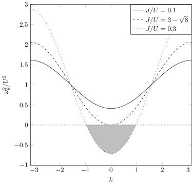
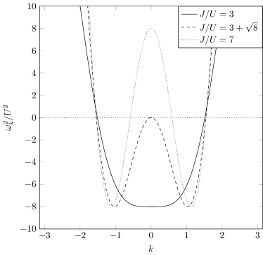
Figure 1: Dispersion relation $\omega_{k}^{2}/U^{2}$ in one dimension for different values of $J/U$.

After these preliminaries, let us study a quantum quench from $J=0$ to a finite value $J_{\rm out}<J_{\rm c}$ which is still in the Mott regime. For simplicity, we consider a sudden change of $J(t)=J_{\rm out}\Theta(t)$, but the calculation can easily be generalized to other scenarios. Solving the evolution equations (24)-(26) for this case, we find NS10

$$\langle\hat{h}^{\dagger}_{\mu}\hat{h}_{\nu}\rangle_{\rm quench} = \langle\hat{p}^{\dagger}_{\mu}\hat{p}_{\nu}\rangle_{\rm quench}$$

$$= \frac{1}{N}\sum_{\mathbf{k}}4J^{2}T_{\mathbf{k}}^{2}\,\frac{1-\cos(\omega_{\mathbf{k}}t)}{\omega^{2}_{\mathbf{k}}}\,e^{i\mathbf{k}\cdot(\mathbf{x}_{\mu}-\mathbf{x}_{\nu})}\;,$$

and

$$\langle\hat{h}^{\dagger}_{\mu}\hat{p}_{\nu}\rangle_{\rm quench} = \frac{i}{N}\sum_{\mathbf{k}}\sqrt{2}JT_{\mathbf{k}}\,\frac{\sin(\omega_{\mathbf{k}}t)}{\omega_{\mathbf{k}}}\,e^{i\mathbf{k}\cdot(\mathbf{x}_{\mu}-\mathbf{x}_{\nu})}$$ (38)

$$+\frac{1}{N}\sum_{\mathbf{k}}\sqrt{2}JT_{\mathbf{k}}(U-3JT_{\mathbf{k}})$$

$$\times\frac{1-\cos(\omega_{\mathbf{k}}t)}{\omega_{\mathbf{k}}^{2}}\,e^{i\mathbf{k}\cdot(\mathbf{x}_{\mu}-\mathbf{x}_{\nu})}\,.$$

The remaining correlation can simply be obtained via $\langle\hat{p}^{\dagger}_{\nu}\hat{h}_{\mu}\rangle=\langle\hat{h}^{\dagger}_{\mu}\hat{p}_{\nu}\rangle^{*}$. The correlator in terms of the original creation and annihilation operators $\hat{b}_{\mu}^{\dagger}$ and $\hat{b}_{\nu}$ is just a linear combination of these correlation functions

$$\langle\hat{b}^{\dagger}_{\mu}\hat{b}_{\nu}\rangle_{\rm quench}=\frac{4JU}{N}\sum_{\mathbf{k}}T_{\mathbf{k}}\,\frac{1-\cos(\omega_{\mathbf{k}}t)}{\omega^{2}_{\mathbf{k}}}\,e^{i\mathbf{k}\cdot(\mathbf{x}_{\mu}-\mathbf{x}_{\nu})}\,.$$ (39)

The quench $J(t)$ can be realized experimentally by decreasing the intensity of the laser field generating the optical lattice (which lowers the potential barrier for tunneling and thus increases $J$). Thus the above prediction should be testable in experiments.

Note that the same expression would apply to a quench from the Mott to the superfluid regime, cf. NS10 . As explained above, in this case the frequencies $\omega_{\mathbf{k}}$ become imaginary for some $\mathbf{k}$ and thus these modes grow exponentially. As a result, the expectation value will quickly be dominated by these fast growing modes and so most of the details of the initial state will become unimportant. Of course, this exponential growth cannot continue forever – after some time, the $1/Z$-expansion breaks down since the quantum fluctuation are too strong and the growth will saturate.

VI Equilibration

However, in the following, we shall study a quench within the Mott regime. In this case, all frequencies are real $\omega_{\mathbf{k}}\in\mathbb{R}$ and thus there is no exponential growth – all modes oscillate. For an infinite (or at least extremely large) lattice, the oscillations in (V-39) average out for sufficiently large times $t$ and thus these observables approach a quasi-equilibrium value

$$\langle\hat{h}^{\dagger}_{\mu}\hat{h}_{\nu}\rangle_{\rm equil} = \langle\hat{p}^{\dagger}_{\mu}\hat{p}_{\nu}\rangle_{\rm equil}$$

$$= \frac{1}{N}\sum_{\mathbf{k}}\frac{4J^{2}T_{\mathbf{k}}^{2}}{\omega^{2}_{\mathbf{k}}}\,e^{i\mathbf{k}\cdot(\mathbf{x}_{\mu}-\mathbf{x}_{\nu})}\;,$$

$$\langle\hat{h}^{\dagger}_{\mu}\hat{p}_{\nu}\rangle_{\rm equil} = \langle\hat{p}^{\dagger}_{\mu}\hat{h}_{\nu}\rangle_{\rm equil}$$

$$= \frac{1}{N}\sum_{\mathbf{k}}\sqrt{2}JT_{\mathbf{k}}\,\frac{U-3JT_{\mathbf{k}}}{\omega_{\mathbf{k}}^{2}}e^{i\mathbf{k}\cdot(\mathbf{x}_{\mu}-\mathbf{x}_{\nu})}\,.$$

The quasi-equilibrium values for the local (on-site) particle and hole probabilities can be derived in complete analogy to the previous case

$$\langle\hat{p}^{\dagger}_{\mu}\hat{p}_{\mu}\rangle_{\rm equil}=\langle\hat{h}_{\mu}\hat{h}^{\dagger}_{\mu}\rangle_{\rm equil}=\frac{1}{N}\sum_{\mathbf{k}}\frac{4J^{2}T_{\mathbf{k}}^{2}}{\omega^{2}_{\mathbf{k}}}\,.$$ (42)

Again, it turn out that the result coincides with Eq. (VI) after setting $\nu=\mu$. For the explicit example of a Bose-Hubbard model on a three-dimensional cubic lattice after a quench according to $J/U=0\to 0.14$, the time dependences from Eqs. (V) and (38) are plotted in Fig. 2.

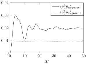
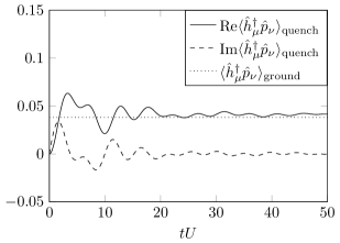
Figure 2: Time-dependence of the depletion $\langle\hat{p}_{\mu}^{\dagger}\hat{p}_{\mu}\rangle$ and the nearest-neighbor correlations functions $\langle\hat{h}_{\mu}^{\dagger}\hat{p}_{\nu}\rangle$ and $\langle\hat{p}_{\mu}^{\dagger}\hat{p}_{\nu}\rangle$ in three dimensions after the quench within the Mott phase $J/U=0\to 0.14$ in comparison to their ground-state values. After quasi-equilibration, $\langle\hat{p}_{\mu}^{\dagger}\hat{p}_{\nu}\rangle_{\mathrm{quench}}$ and $\langle\hat{p}_{\mu}^{\dagger}\hat{p}_{\nu}\rangle_{\mathrm{ground}}$ as well as $\langle\hat{p}_{\mu}^{\dagger}\hat{p}_{\mu}\rangle_{\mathrm{quench}}$ and $\langle\hat{p}_{\mu}^{\dagger}\hat{p}_{\mu}\rangle_{\mathrm{ground}}$ differ roughly by a factor of two.

Having found that the observables considered above approach a quasi-equilibrium state, it is natural to ask the question of thermalization. As explained in the Introduction, this is one of the major unsolved questions (or rather a set of questions) in quantum many-body theory KWE11 ; GME11 ; EHKKMWW09 ; KISD11 ; BCH11 . Even though we cannot settle this question here, we can compare the quasi-equilibrium values obtained above with a thermal state. To this end, we derive the thermal density matrix $\hat{\rho}_{\beta}$ corresponding to a given temperature $k_{\rm B}T=1/\beta$. Using the grand canonical ensemble, the thermal density operator reads

$$\hat{\rho}_{\beta}=\frac{e^{-\beta(\hat{H}-\mu\hat{N})}}{\,{\rm Tr}\{e^{-\beta(\hat{H}-\mu\hat{N})}\}}\,,$$ (43)

where chemical potential $\mu$ will be chosen such that the filling is equal to unity. For small values of $J/U$, we can employ strong-coupling perturbation theory, i.e., an expansion in powers of $J/U$. It is useful to introduce the operator CFMSE08 ; FCMSE08

$$\hat{R}(\beta)=e^{\beta\hat{H}_{0}}e^{-\beta(\hat{H}_{0}+\hat{H}_{1})}\,,$$ (44)

where $\hat{H}_{0}$ is the diagonal on-site part of the grand canonical Hamiltonian $\hat{H}-\mu\hat{N}$ and $\hat{H}_{1}$ is the hopping term. This operator satisfies the differential equation

$$\partial_{\beta}\hat{R}(\beta)=-\hat{H}_{1}(\beta)\hat{R}(\beta)\,,$$ (45)

where $\hat{H}_{1}(\beta)=e^{\beta\hat{H}_{0}}\hat{H}_{1}e^{-\beta\hat{H}_{0}}$. In analogy to time-dependent perturbation theory, the operator $\hat{R}$ can be calculated perturbatively by integrating this equation with respect to $\beta$. In first-order perturbation expansion (in $J/U$), we have (see also Ref. CFMSE08 )

$$\hat{\rho}_{\beta}=\frac{e^{-\beta\hat{H}_{0}}}{{\mathfrak{Z}}_{0}}\left(1+\frac{J}{Z}\sum_{\mu\nu}T_{\mu\nu}\,\hat{b}^{\dagger}_{\mu}\frac{e^{\beta U(\hat{n}_{\mu}-\hat{n}_{\nu})}-1}{U(\hat{n}_{\mu}-\hat{n}_{\nu})}\,\hat{b}_{\nu}\right)$$ (46)

with ${\mathfrak{Z}}_{0}={\,{\rm Tr}\{e^{-\beta\hat{H}_{0}}\}}$. Obviously, the correction to first order in $J/U$ does not affect the one-point density matrix $\hat{\rho}_{\mu}$ but the two-point correlations. Thus, we find that the quasi-equilibrium state of the one-point density matrix $\hat{\rho}_{\mu}$ can indeed be described by a thermal state provided that we choose the chemical potential as $\mu=U/2$ which gives

$$\hat{\rho}_{\mu}(\beta) \approx \frac{e^{-\beta U/2}}{2}\,\left|0\right>_{\mu}\!\left<0\right|+\left(1-e^{-\beta U/2}\right)\left|1\right>_{\mu}\!\left<1\right|$$ (47)

$$+\frac{e^{-\beta U/2}}{2}\,\left|2\right>_{\mu}\!\left<2\right|\,.$$

The particular value $\mu=U/2$ of the chemical potential ensures that (in first order thermal perturbation theory) we have on average one particle per lattice site and the particle-hole symmetry $\langle\hat{p}_{\mu}^{\dagger}\hat{p}_{\mu}\rangle=\langle\hat{h}_{\mu}^{\dagger}\hat{h}_{\mu}\rangle$. To obtain the correct probabilities, we have to select the temperature according to

$$e^{-\beta U/2}=2\langle\hat{p}^{\dagger}_{\mu}\hat{p}_{\mu}\rangle_{\rm equil}=\frac{8J^{2}}{N}\sum_{\mathbf{k}}\frac{T_{\mathbf{k}}^{2}}{\omega^{2}_{\mathbf{k}}}=\,{\cal O}(1/Z)\,,$$ (48)

which can be deduced from Eqs. (42) and (47). Since the depletion is small $\langle\hat{p}^{\dagger}_{\mu}\hat{p}_{\mu}\rangle=\,{\cal O}(1/Z)$, we obtain a low effective temperature which scales as $T=\,{\cal O}(U/\ln Z)$. Accordingly, consistent with our $1/Z$-expansion, we can neglect higher Boltzmann factors such as $e^{-\beta U}$.

VII Correlations

Of course, the fact that the one-point density matrix $\hat{\rho}_{\mu}$ can be described (within our limits of accuracy) by a thermal state does not imply that the same is true for the correlations. To study this point, let us calculate the thermal two-point correlator from (46). To first order in $J/U$ and $1/Z=\,{\cal O}(e^{-\beta U}/2)$, we find

$$\langle\hat{h}^{\dagger}_{\mu}\hat{p}_{\nu}\rangle_{\beta} = \langle\hat{p}^{\dagger}_{\mu}\hat{h}_{\nu}\rangle_{\beta}=\frac{\sqrt{2}JT_{\mu\nu}}{ZU}$$ (49)

$$+\,{\cal O}(J^{2})+\,{\cal O}(1/Z^{2})\,,$$

while $\langle\hat{h}^{\dagger}_{\mu}\hat{h}_{\nu}\rangle_{\beta}$ and $\langle\hat{p}^{\dagger}_{\mu}\hat{p}_{\nu}\rangle_{\beta}$ vanish (to first order in $J/U$). If we compare this to the quasi-equilibrium value $\langle\hat{h}^{\dagger}_{\mu}\hat{p}_{\nu}\rangle_{\rm equil}$ in (VI), we find that they coincide to first order in $J/U$

$$\langle\hat{h}^{\dagger}_{\mu}\hat{p}_{\nu}\rangle_{\rm equil} = \langle\hat{p}^{\dagger}_{\mu}\hat{h}_{\nu}\rangle_{\rm equil}=\frac{\sqrt{2}JT_{\mu\nu}}{ZU}$$ (50)

$$+\,{\cal O}(J^{2})+\,{\cal O}(1/Z^{2})\,.$$

This is perhaps not too surprising since the same value can be obtained from the ground-state fluctuations $\langle\hat{h}^{\dagger}_{\mu}\hat{p}_{\nu}\rangle_{\rm ground}=\langle\hat{p}^{\dagger}_{\mu}\hat{h}_{\nu}\rangle_{\rm ground}$ in (IV) after expanding them to first order in $J/U$. Due to the low effective temperature $T=\,{\cal O}(U/\ln Z)$, the lowest Boltzmann factor is suppressed by $e^{-\beta U/2}=\,{\cal O}(1/Z)$. As a consequence, because the correlations are small $\,{\cal O}(1/Z)$, their finite-temperature corrections are even smaller $\,{\cal O}(1/Z^{2})$, and thus can be neglected.

The same is true for the other correlations $\langle\hat{h}^{\dagger}_{\mu}\hat{h}_{\nu}\rangle=\langle\hat{p}^{\dagger}_{\mu}\hat{p}_{\nu}\rangle$. All of them: the ground-state correlators $\langle\hat{h}^{\dagger}_{\mu}\hat{h}_{\nu}\rangle_{\rm ground}=\langle\hat{p}^{\dagger}_{\mu}\hat{p}_{\nu}\rangle_{\rm ground}$ in (IV), the quasi-equilibrium correlators $\langle\hat{h}^{\dagger}_{\mu}\hat{h}_{\nu}\rangle_{\rm equil}=\langle\hat{p}^{\dagger}_{\mu}\hat{p}_{\nu}\rangle_{\rm equil}$ in (VI), as well as the thermal correlators $\langle\hat{h}^{\dagger}_{\mu}\hat{h}_{\nu}\rangle_{\beta}$ and $\langle\hat{p}^{\dagger}_{\mu}\hat{p}_{\nu}\rangle_{\beta}$ vanish to first order in $J/U$. Therefore, to first order in $J/U$ and $1/Z$, the thermal state can describe the observables under consideration. However, going to the next order in $J$, this description breaks down. This failure can even be shown without explicitly calculating $\hat{R}(\beta)$ up to second order. If we compare the quasi-equilibrium correlators (VI)

$$\langle\hat{h}^{\dagger}_{\mu}\hat{h}_{\nu}\rangle_{\rm equil} = \langle\hat{p}^{\dagger}_{\mu}\hat{p}_{\nu}\rangle_{\rm equil}=\frac{4J^{2}}{U^{2}Z^{2}}\sum_{\kappa}T_{\mu\kappa}T_{\kappa\nu}$$ (51)

$$+\,{\cal O}(J^{3})+\,{\cal O}(1/Z^{2})\,,$$

with the ground-state correlations in (IV), expanded to the same order in $J$

$$\langle\hat{h}^{\dagger}_{\mu}\hat{h}_{\nu}\rangle_{\rm ground} = \langle\hat{p}^{\dagger}_{\mu}\hat{p}_{\nu}\rangle_{\rm ground}=\frac{2J^{2}}{U^{2}Z^{2}}\sum_{\kappa}T_{\mu\kappa}T_{\kappa\nu}$$ (52)

$$+\,{\cal O}(J^{3})+\,{\cal O}(1/Z^{2})\,,$$

we find a discrepancy by a factor of two footnote-lattice-structure . I.e., after the quench, these correlations settle down to a value which is twice as large as in the ground state (see Fig. 2). This factor of two has already been found elsewhere in the context of standard time-dependent and time-independent perturbation theory, see also MK09 . This is incompatible with the small Boltzmann factors $e^{-\beta U/2}=\,{\cal O}(1/Z)$ and would require a comparably large effective temperature $T=\,{\cal O}(U)$ instead of $T=\,{\cal O}(U/\ln Z)$. However, such a large effective temperature $T=\,{\cal O}(U)$ is inconsistent with the small on-site depletion (48).

This distinction between local observables (which become approximately thermal) and non-local correlations (which are incompatible with this thermal state) has already been observed in other scenarios using different approaches. For the Bose-Hubbard model, quenches from the superfluid phase to the Mott state at finite values of $J$ and $U$ have been studied in Ref. KLA07 , where a significant dependence on the final values of $J$ and $U$ has been observed: For large values of the final $U$, the (quasi) equilibrated correlations deviate significantly from a thermal state, whereas this deviation is not pronounced for smaller values. In contrast, a quench between the two exactly solvable cases $J=0$ on the one hand and $U=0$ on the other hand has been studied in Ref. CDEO08 . This case can be solved exactly and consistent with the existence of the conservation laws (as mentioned in the Introduction), only partial thermalization is observed. Further studies have been devoted to bosonic superlattices (see, e.g., Ref. CFMSE08 ) and fermionic systems (see the discussion at the end of Section XII), for example. Unfortunately, a general and unifying understanding of all these non-equilibrium phenomena is still missing.

VIII Second Order in $1/Z$

So far, we have only considered the first order in $1/Z$. Now let us discuss the effect of higher orders by means of a few examples. Unfortunately, the complete derivation is rather lengthy and cannot be given here, it will be presented elsewhere elsewhere .

Let us go back to the derivation from (10) to (12) and include $1/Z^{2}$ corrections. To achieve this level of accuracy, we should not replace the exact one-point density matrix $\hat{\rho}_{\mu}$ by it lowest-order approximation $\hat{\rho}_{\mu}^{0}$ but include its first-order corrections in (35), i.e., the quantum depletion $f_{0}=\,{\rm Tr}\{\hat{\rho}_{\mu}|0\rangle_{\mu}\langle 0|\}=\langle\hat{h}_{\mu}\hat{h}^{\dagger}_{\mu}\rangle=\,{\cal O}(1/Z)$ of the unit filling (Mott) state in Eq. (35). This results in a renormalization of the eigenfrequency

$$\omega_{\mathbf{k}}^{\rm ren}=\sqrt{U^{2}-6JT_{\mathbf{k}}(1-3f_{0})+J^{2}T_{\mathbf{k}}^{2}(1-3f_{0})^{2}}\,,$$ (53)

Since the net effect can roughly be understood as a reduction of the effective hopping rate $J^{\rm ren}=J(1-3f_{0})$, it is easy to visualize that this implies also a decrease of the effective propagation velocity.

There are also other $1/Z^{2}$ corrections in (12) such as the three-point correlator $\hat{\rho}^{\rm corr}_{\mu\nu\kappa}$ but they act as source terms and do not affect the eigenfrequency (at second order). However, there are other quantities where these source terms are crucial. In particular, we consider two-point correlation functions which vanish to first order in $1/Z$, in contrast to contributions such as $\langle\hat{b}^{\dagger}_{\mu}\hat{b}_{\nu}\rangle$ discussed above. One important example is the particle-number correlation, i.e., $\langle\hat{n}_{\mu}\hat{n}_{\nu}\rangle-\langle\hat{n}_{\mu}\rangle\langle\hat{n}_{\nu}\rangle$. After a somewhat lengthy calculation, we find for the ground-state correlations

$$\langle\hat{n}_{\mu}\hat{n}_{\nu}\rangle-\langle\hat{n}_{\mu}\rangle\langle\hat{n}_{\nu}\rangle=$$

$$\frac{2}{N^{2}}\sum_{\mathbf{p},\mathbf{q}}e^{i(\mathbf{p}+\mathbf{q})\cdot(\mathbf{x}_{\mu}-\mathbf{x}_{\nu})}\left(f^{11}_{\mathbf{p}}f^{11}_{\mathbf{q}}-f^{12}_{\mathbf{p}}f^{21}_{\mathbf{q}}\right)\,,$$ (54)

where $f^{12}_{\mathbf{p}},f^{21}_{\mathbf{p}}$ and $f^{11}_{\mathbf{p}}$ are given through the relations (30). Note that the above result is non-perturbative in $J/U$, see, for example, the non-polynomial dependence of $\omega_{\mathbf{k}}$ on $J$.

As a related example, the parity correlator reads

$$\langle(-1)^{\hat{n}_{\mu}}(-1)^{\hat{n}_{\nu}}\rangle-\langle(-1)^{\hat{n}_{\mu}}\rangle\langle(-1)^{\hat{n}_{\mu}}\rangle=$$

$$\frac{8}{N^{2}}\sum_{\mathbf{p},\mathbf{q}}e^{i(\mathbf{p}+\mathbf{q})\cdot(\mathbf{x}_{\mu}-\mathbf{x}_{\nu})}\left(f^{11}_{\mathbf{p}}f^{11}_{\mathbf{q}}+f^{12}_{\mathbf{p}}f^{21}_{\mathbf{q}}\right)\,.$$ (55)

In analogy to the previous Section, we can also study the correlations after a quantum quench with $J(t)=J\Theta(t)$. Again, there are no contributions to the particle-number and parity correlations in first order $1/Z$ – but, to second order $1/Z$, we find formally the same expressions as in the static case (VIII) and (VIII) where $f^{12}_{\mathbf{p}}(t)$, $f^{21}_{\mathbf{p}}(t)$, and $f^{11}_{\mathbf{p}}(t)$ are now given by equations (V) and (38). The parity correlations after a quench have been experimentally observed in a one-dimensional setup CBPE12 . Although the hierarchical expansion relies on a large coordination number, we find qualitative agreement between the theoretical prediction (VIII) for $Z=2$ and the results from CBPE12 . For large times $t$ and distances $\mathbf{x}_{\mu}-\mathbf{x}_{\nu}$, we may estimate the integrals over $\mathbf{p}$ and $\mathbf{q}$ in the expressions (VIII) and (VIII) via the stationary-phase or saddle-point approximation. The dominant contributions stem from the momenta satisfying the saddle-point condition

$$\nabla_{\mathbf{k}}\left[\mathbf{k}\cdot(\mathbf{x}_{\mu}-\mathbf{x}_{\nu})\pm\omega_{\mathbf{k}}t\right]=0\,.$$ (56)

Thus their structure is determined by the group velocity $\mathbf{v}_{\mathbf{k}}=\nabla_{\mathbf{k}}\omega_{\mathbf{k}}$. If the equation $\mathbf{x}_{\mu}-\mathbf{x}_{\nu}=\pm\mathbf{v}_{\mathbf{k}}t$ has a real solution $\mathbf{k}$, i.e., if the distance $\mathbf{x}_{\mu}-\mathbf{x}_{\nu}$ can be covered in the time $t$ with the group velocity $\mathbf{v}_{\mathbf{k}}$, then we get a stationary-phase solution – otherwise the integral will be exponentially suppressed (i.e., the saddle point $\mathbf{k}$ becomes complex). For a given direction in ${\bf k}$-space, the maximum group velocity determines the maximum propagation speed of correlations, i.e., the effective light cone. In a hypercubic lattice in $D$ dimensions with small $J$, for example, it is given by $v_{\rm max}\approx 3J/D$ along the lattice axes and by $v_{\rm max}\approx 3J/\sqrt{D}$ along the diagonal (where all the components of ${\bf v}_{\rm max}$ are equal to each other). A similar result has been obtained in Ref. BPCK12 for the one-dimensional Bose-Hubbard model. For an experimental realization, see, e.g., Ref. CBPE12 .

IX Exact numerical results

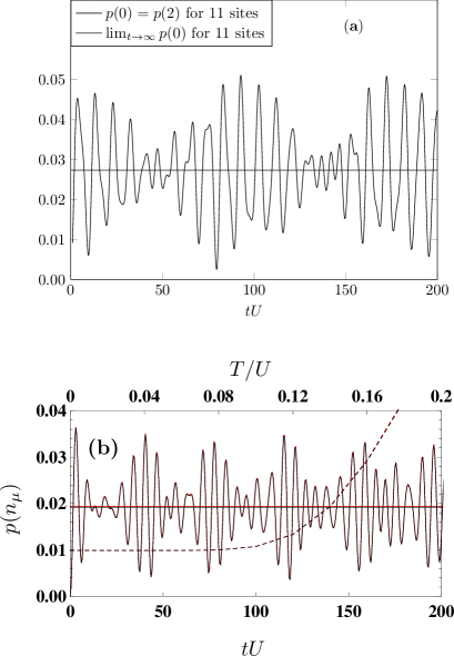
Figure 3: (Color online) Time evolution of the probabilities to have zero (red) and two (black) particles after quench from $J/U=0$ to $J/U=0.1$ in a one-dimension lattice of $11$ sites with $n=1$ atom per site. Straight horizontal lines show the values averaged over an infinite evolution time. Top (a): first order of $1/Z$ expansion, see Eqs. (V),  (VI). Bottom (b): exact diagonalization. Dashed lines: Probabilities to have $n_{\mu}=0$ (red), $2$ (black) atoms in a thermal state at $J/U=0.1$ as a function of temperature $T$. Note the different scales for the time $t$ and temperature $T$ dependences.

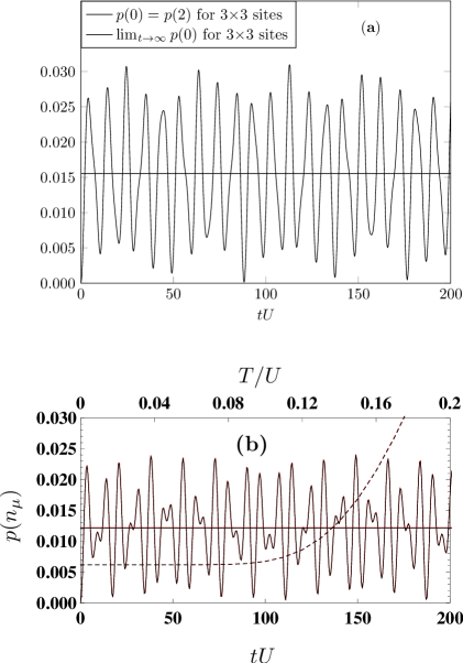
Figure 4: (Color online) Time evolution of the probabilities to have zero (red) or two (black) particles after quench from $J/U=0$ to $J/U=0.1$ in a two-dimension lattice of $3\times 3$ sites with $n=1$ atom per site. Straight horizontal lines show the values averaged over an infinite evolution time. Top (a): first order of $1/Z$ expansion, see Eqs. (V),  (VI). Bottom (b): exact diagonalization. Dashed lines: Probabilities to have $n_{\mu}=0$ (red), $2$ (black) atoms in a thermal state at $J/U=0.1$ as a function of temperature $T$. Note the different scales for the time $t$ and temperature $T$ dependences.

In order to test the quality of our $1/Z$ expansion, we compare the predictions of our first-order calculations with exact numerical results for the probabilities $p(n_{\mu})=\left<n\right|\hat{\rho}_{\mu}\left|n\right>$ and correlation functions $\langle\hat{b}^{\dagger}_{\mu}\hat{b}_{\nu}\rangle$ in one- and two-dimensional finite lattices. They are obtained by full diagonalization of the Bose-Hubbard Hamiltonian with periodic boundary conditions without any truncation of the Hilbert space. This allows us to calculate exactly the complete time evolution of any quantity as well as their mean values averaged over an infinite time. The initial state can be arbitrary and in the calculations presented below it was chosen in the form described by Eq. (15). The full diagonalization provides also a possibility of exact calculations of the thermal averages.

The time evolution of the probabilities $p(n_{\mu}=0)$ and $p(n_{\mu}=2)$, which are by definition equivalent to the quantities $\langle\hat{h}_{\mu}\hat{h}^{\dagger}_{\mu}\rangle$ and $\langle\hat{p}^{\dagger}_{\mu}\hat{p}_{\mu}\rangle$ considered in the previous sections, is shown in Figs. 3 and 4 for one- and two-dimensional lattices, respectively. Due to finite-size effects (see also Ref. GR10 ), these probabilities oscillate around their averaged values shown by straight horizontal lines. For the chosen value of $J/U=0.1$, the behavior of $p(0)$ is almost indistinguishable from that of $p(2)$, consistent with the $1/Z$-expansion. The probabilities for thermal equilibrium states corresponding to the final value of $J/U$ (depending on their temperature $T$) are also plotted for comparison. We observe that the time-averaged values of the probabilities correspond to an effective temperature of about $0.14~{}U$, which is consistent with the results of Sec. VI. Furthermore, we find that, in a one-dimensional lattice, our $1/Z$-approach underestimates the typical frequency scales and overestimates the characteristic amplitudes of the probabilities by roughly the same factor of $\approx 1.4$. This might be an indication of the effective renormalization of the hopping rate $J^{\rm ren}=J(1-3f_{0})$ by the quantum fluctuations discussed in the previous section (which are neglected to first order in $1/Z$). In two dimensions, this discrepancy is still present – albeit noticeably smaller. In total, we see that the quantum fluctuations in two dimensions are smaller than in one dimension – and that our $1/Z$-expansion becomes better (as one would expect).

The time dependence of the correlation functions $\langle\hat{b}^{\dagger}_{\mu}\hat{b}_{\nu}\rangle$ presented in Figs. 5, 6 displays similar oscillating character and the comparison of the $1/Z$-expansion with exact diagonalization reveals the same characteristic features. In the one-dimensional lattice, their time-averaged values can again be approximately described by an effective temperature of about $0.2~{}U$, but this temperature is already significantly larger than that for the probabilities $p(n_{\mu})$. In contrast, in the two-dimensional case, the time-averaged correlation functions cannot be described at all by a thermal state, see Fig. 6 since are larger than the thermal correlations at any temperature. This failure of an effective temperature in the two-dimensional system is consistent with the result obtained within the $1/Z$-expansion in Sec. VI. Note that the situation considered here is quite different from a quench across the critical point (i.e., Mott-superfluid or superfluid-Mott) for which qualitatively different results have been obtained in KLA07 ; GR10 , for example.

In general, we come to the conclusion that our $1/Z$-expansion agrees qualitatively surprisingly well with exact diagonalization even in one and two dimensions, although the values of $1/Z=0.5$ and $0.25$ are not so small. Furthermore, we observe that the quantitative agreement between our $1/Z$-expansion and the numerical results becomes better when going from one to two dimensions, as one would expect.

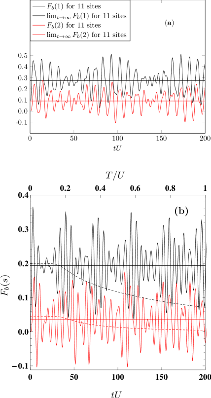
Figure 5: (Color online) Correlation function $F_{b}(s)=\langle\hat{b}^{\dagger}_{\mu}\hat{b}_{\nu}\rangle$ for nearest neighbors $s=1$ [the solid black (upper) curve] and next-to-nearest neighbors $s=2$ [the solid red (lower) curve] after a quench from $J/U=0$ to $J/U=0.1$ in a one-dimension lattice of $11$ sites with $n=1$ atom per site. Straight horizontal lines show the values averaged over an infinite evolution time. Top (a): first order of $1/Z$ expansion, see Eqs. (39),  (VI), (VI). Bottom (b) exact diagonalization. Dashed lines in panel (b): $F_{b}(1)$ [black (upper)] and $F_{b}(2)$ [red (lower)] in a thermal state at $J/U=0.1$ as functions of temperature $T$. Note the different scales for the time $t$ and temperature $T$ dependences.

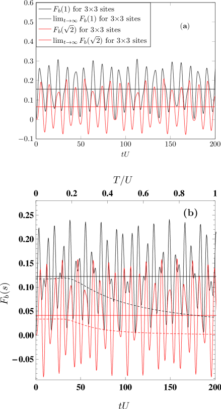
Figure 6: (Color online) Correlation function $F_{b}(s)=\langle\hat{b}^{\dagger}_{\mu}\hat{b}_{\nu}\rangle$ for nearest neighbors $s=1$ [the solid black (upper) curve] and next-to-nearest (diagonal) neighbors $s=\sqrt{2}$ [the solid red (lower) curve] after a quench from $J/U=0$ to $J/U=0.1$ in a two-dimension lattice of $3\times 3$ sites with $n=1$ atom per site. Straight horizontal lines show the values averaged over an infinite evolution time. Top (a): first order of $1/Z$ expansion, see Eqs. (39),  (VI), (VI). Bottom (b): exact diagonalization. Dashed lines in panel (b): $F_{b}(1)$ [black (upper)] and $F_{b}(\sqrt{2})$ [red (lower)] in a thermal state at $J/U=0.1$ as functions of temperature $T$. Note the different scales for the time $t$ and temperature $T$ dependences.

X Fermi-Hubbard model

Now, after having studied the bosonic case, let us investigate the Fermi-Hubbard model H63 ; EFGKK05 ; F91 . We shall find many similarities to the Bose-Hubbard model – but also crucial differences. The Hamiltonian reads

$$\hat{H}=-\frac{J}{Z}\sum_{\mu\nu,s}T_{\mu\nu}\hat{c}_{\mu,s}^{\dagger}\hat{c}_{\nu,s}+U\sum_{\mu}\hat{n}_{\mu}^{\uparrow}\hat{n}_{\mu}^{\downarrow}\,.$$ (57)

The nomenclature is the same as in the bosonic case (1) but with an additional spin label $s$ which can assume two values $s=\uparrow$ or $s=\downarrow$. In the following, we consider the case of half-filling $\langle\hat{n}_{\mu}^{\uparrow}+\hat{n}_{\mu}^{\downarrow}\rangle=1$ where half the particles are in the $s=\uparrow$ state and the other have $s=\downarrow$. Note that the total particle numbers $\hat{N}^{\uparrow}=\sum_{\mu}\hat{n}_{\mu}^{\uparrow}$ and $\hat{N}^{\downarrow}=\sum_{\mu}\hat{n}_{\mu}^{\downarrow}$ for each spin species are conserved separately $[\hat{H},\hat{N}^{\uparrow}]=[\hat{H},\hat{N}^{\downarrow}]=0$. The creation and annihilation operators satisfy the fermionic anti-commutation relations

$$\left\{\hat{c}_{\nu,a},\hat{c}_{\mu,b}^{\dagger}\right\}=\delta_{\mu\nu}\delta_{ab}\;,\,\left\{\hat{c}_{\nu,a},\hat{c}_{\mu,b}\right\}=\left\{\hat{c}_{\nu,a}^{\dagger},\hat{c}_{\mu,b}^{\dagger}\right\}=0\,.$$ (58)

The fermionic nature of the particles has important consequences. For example, let us estimate the expectation value of the hopping Hamiltonian $\hat{H}_{J}$. Introducing the “coarse-grained” operator

$$\hat{c}_{\mu,s}^{\Sigma}=\frac{1}{\sqrt{Z}}\sum_{\nu}T_{\mu\nu}\hat{c}_{\nu,s}\,,$$ (59)

we may write the expectation value of the tunneling energy $\hat{H}_{J}$ per lattice site for one spin species $s$ as $-J\langle\hat{c}_{\mu,s}^{\dagger}\hat{c}_{\mu,s}^{\Sigma}\rangle/\sqrt{Z}$. This expectation value can be interpreted as a scalar product of the two vectors $\hat{c}_{\mu,s}\left|\Psi\right>$ and $\hat{c}_{\mu,s}^{\Sigma}\left|\Psi\right>$ and hence it is bounded by

$$\left|\left<\Psi\right|\hat{c}_{\mu,s}^{\dagger}\hat{c}_{\mu,s}^{\Sigma}\left|\Psi\right>\right|\leq||\hat{c}_{\mu,s}\left|\Psi\right>||\cdot||\hat{c}_{\mu,s}^{\Sigma}\left|\Psi\right>||\,.$$ (60)

Inserting $||\hat{c}_{\mu,s}\left|\Psi\right>||^{2}=\left<\Psi\right|\hat{c}_{\mu,s}^{\dagger}\hat{c}_{\mu,s}\left|\Psi\right>=\left<\Psi\right|\hat{n}_{\mu,s}\left|\Psi\right>$, we get the expectation value of the number operator $\hat{n}_{\mu,s}$. In contrast to the bosonic case, this operator is bounded and thus we find $||\hat{c}_{\mu,s}\left|\Psi\right>||\leq 1$. Furthermore, the operator $\hat{c}_{\mu,s}^{\Sigma}$ in (59) obeys the same anti-commutation relations (58) and thus we find $||\hat{c}_{\mu,s}^{\Sigma}\left|\Psi\right>||\leq 1$ in complete analogy. Consequently, the absolute value of the tunneling energy per lattice site is below $2J/\sqrt{Z}$, i.e., decreases for large $Z$.

The above result implies that the interaction term $\propto U$ always dominates (except in the trivial case $U=0$) in the limit $Z\to\infty$ under consideration. Hence, we are in the strongly interacting Mott regime and do not find anything analogous to the Mott–superfluid transition as in the bosonic case. Note that often MV89 ; F99 a different $Z$-scaling is considered, where the hopping term scales with $J/\sqrt{Z}$ instead of $J/Z$ as in (57). Using this $J/\sqrt{Z}$ scaling, one can study the transition from the Mott state to a metallic state which is supposed to occur at a critical value of $J$ where – roughly speaking – the hopping term starts to dominate over the interaction term. However, this transition is not as well understood as the Mott–superfluid transition in the bosonic case. With our $J/Z$-scaling in (57), we study a different corner of the phase space where we can address question such as tunneling in tilted lattices and equilibration vs thermalization etc.

X.1 Symmetries and Degeneracy

In addition to the usual invariances already known from the bosonic case, the Fermi-Hubbard model has some more symmetries. For example, the particle-hole symmetry $\hat{c}_{\mu,s}^{\dagger}\leftrightarrow\hat{c}_{\mu,s}$ and thus $\hat{n}_{\mu,s}=\hat{c}_{\mu,s}^{\dagger}\hat{c}_{\mu,s}\leftrightarrow\hat{\bar{n}}_{\mu,s}=\hat{c}_{\mu,s}\hat{c}_{\mu,s}^{\dagger}=1-\hat{n}_{\mu,s}$ is no longer an effective approximate symmetry, but becomes exact (for the case of half-filling considered here).

Furthermore, there is an effective $SU(2)$-symmetry corresponding to the spin degrees of freedom. To specify this, let us introduce the effective spin operators

$$\hat{S}_{\mu}^{z}=\frac{1}{2}\sum\limits_{ab}\hat{c}_{\mu,a}^{\dagger}\,\sigma^{z}_{ab}\,\hat{c}_{\mu,b}=\frac{1}{2}\left(\hat{n}_{\mu}^{\uparrow}-\hat{n}_{\mu}^{\downarrow}\right)\,,$$ (61)

and analogously $\hat{S}_{\mu}^{x}=\sum_{ab}\hat{c}_{\mu,a}^{\dagger}\sigma^{x}_{ab}\hat{c}_{\mu,b}/2$ as well as $\hat{S}_{\mu}^{y}=\sum_{ab}\hat{c}_{\mu,a}^{\dagger}\sigma^{y}_{ab}\hat{c}_{\mu,b}/2$ where $\sigma^{x,y,z}_{ab}$ are the usual Pauli spin matrices. These operators satisfy the usual spin, i.e., $SU(2)$, commutation relations and the Fermi-Hubbard Hamiltonian (57) is invariant under global $SU(2)$ rotations generated by the total spin operators $\hat{\mathbf{S}}_{\rm tot}=\sum_{\mu}\hat{\mathbf{S}}_{\mu}$.

In the case of zero hopping $J=0$, this global $SU(2)$ invariance even becomes a local symmetry, i.e., we may perform a spin rotation at each site without changing the energy. As a result, the ground state (at half filling) is highly degenerate for $J=0$ in contrast to the Bose-Hubbard model (at integer filling). This degeneracy can be lifted by an additional staggered magnetic field (see XI.1) and is related to the spin modes which become arbitrarily soft for small $J$. In this limit $J\ll U$, their dynamics can be described by an effective Hamiltonian, which is basically the Heisenberg model

$$\hat{H}=\frac{2J^{2}}{Z^{2}U}\sum_{\mu\nu}T_{\mu\nu}\,\hat{\mathbf{S}}_{\mu}\cdot\hat{\mathbf{S}}_{\nu}\,,$$ (62)

with an effective anti-ferromagnetic coupling constant of order $1/Z^{2}$. This effective Hamiltonian describes the Fermi-Hubbard Hamiltonian (57) for half-filling in the low-energy sub-space where we have one particle per site, but with a variable spin $\hat{\mathbf{S}}_{\mu}$.

In order to avoid complications such as frustration for the anti-ferromagnetic Heisenberg model (62), we assume a bipartite lattice – i.e., we can divide the total lattice into two sub-lattices $\cal A$ and $\cal B$ such that, for each site in $\mu\in\cal A$, all the neighboring sites $\nu$ belong to $\cal B$ and vice versa. In this case, the ground state of the Heisenberg model (62) approaches the Néel state for large $Z$

$$\hat{\rho}_{\rm Neel}=\bigotimes_{\mu\in\cal A}\bigotimes_{\nu\in\cal B}\hat{n}_{\mu}^{\downarrow}\,\hat{\bar{n}}_{\mu}^{\uparrow}\,\hat{n}_{\nu}^{\uparrow}\,\hat{\bar{n}}_{\nu}^{\downarrow}\,,$$ (63)

which is just the state with exactly one particle per site, but in alternating spin states, i.e., $s=\downarrow$ for $\mu\in\cal A$ and $s=\uparrow$ for $\nu\in\cal B$. Note that $\hat{n}_{\mu}^{\downarrow}$ is the projector on the $\left|1\right>_{\mu}^{\downarrow}$ state $\hat{n}_{\mu}^{\downarrow}=\left|1^{\downarrow}\right>_{\mu}\left<1^{\downarrow}\right|$ while $\hat{\bar{n}}_{\mu}^{\uparrow}$ projects on the $\left|0\right>_{\mu}^{\uparrow}$ state etc. As usual, this state (63) breaks the original symmetry group of the Hamiltonian (57) containing particle-hole symmetry, $SU(2)$ invariance, and translational symmetry, down to a sub-group, which includes invariance under a combined spin-flip and particle-hole exchange etc.

Let us stress that the Néel state (63) is only the lowest-order approximation of the real ground state of the Heisenberg model (62), there are quantum spin fluctuations of order $\,{\cal O}(1/Z)$. These quantum spin fluctuations do not vanish in the limit $J\to 0$ since $J$ only appears in the overall pre-factor in front of the Heisenberg Hamiltonian (62) while the internal structure remains the same. Only after adding a suitable staggered magnetic field (see XI.1), the Néel state (63) is the exact unique ground state (for $J\to 0$). Either way, in analogy to the bosonic case, we can now use this fully factorizing state (63) as the starting point for our $1/Z$-expansion.

XI Mott-Néel state

Starting with the Néel state (63) as the zeroth order in $1/Z$, let us now derive the first-order corrections. To this end, let us consider the Heisenberg equations of motion

$$i\partial_{t}\hat{c}_{\mu s} = -\frac{J}{Z}\sum_{\kappa\neq\mu}T_{\mu\kappa}\hat{c}_{\kappa s}+U\hat{c}_{\mu s}\hat{n}_{\mu\bar{s}}$$ (64)

$$i\partial_{t}\hat{c}_{\mu s}^{\dagger} = +\frac{J}{Z}\sum_{\kappa\neq\mu}T_{\mu\kappa}\hat{c}^{\dagger}_{\kappa s}-U\hat{c}^{\dagger}_{\mu s}\hat{n}_{\mu\bar{s}}$$ (65)

$$i\partial_{t}\hat{n}_{\mu s} = \frac{J}{Z}\sum_{\kappa\neq\mu}T_{\mu\kappa}\left(\hat{c}_{\kappa s}^{\dagger}\hat{c}_{\mu s}-\hat{c}_{\mu s}^{\dagger}\hat{c}_{\kappa s}\right)$$ (66)

$$= -i\partial_{t}\hat{\bar{n}}_{\mu s}\,,$$

where $\bar{s}$ denotes the spin label opposite to $s$, i.e., either $(s,\bar{s})=(\uparrow,\downarrow)$ or $(s,\bar{s})=(\downarrow,\uparrow)$. If we now insert these evolution equations into the correlation functions $\langle\hat{c}_{\mu a}^{\dagger}\hat{c}_{\nu b}\hat{n}_{\mu\bar{a}}\hat{n}_{\nu\bar{b}}\rangle$, $\langle\hat{c}_{\mu a}^{\dagger}\hat{c}_{\nu b}\hat{\bar{n}}_{\mu\bar{a}}\hat{n}_{\nu\bar{b}}\rangle$, $\langle\hat{c}_{\mu a}^{\dagger}\hat{c}_{\nu b}\hat{n}_{\mu\bar{a}}\hat{\bar{n}}_{\nu\bar{b}}\rangle$, and $\langle\hat{c}_{\mu a}^{\dagger}\hat{c}_{\nu b}\hat{\bar{n}}_{\mu\bar{a}}\hat{\bar{n}}_{\nu\bar{b}}\rangle$, we find that they form a closed set of equations to first order in $1/Z$, where we can neglect three-point correlations

$$i\partial_{t}\langle\hat{c}_{\mu a}^{\dagger}\hat{c}_{\nu b}\hat{n}_{\mu\bar{a}}\hat{n}_{\nu\bar{b}}\rangle=+\frac{J}{Z}T_{\mu\nu}\langle\hat{c}_{\nu a}^{\dagger}\hat{c}_{\nu b}\hat{n}_{\mu\bar{a}}\hat{n}_{\nu\bar{b}}\rangle_{0}$$

$$+\frac{J}{Z}\langle\hat{n}_{\mu\bar{a}}\rangle_{0}\sum_{\kappa\neq\mu,\nu}T_{\mu\kappa}\langle\hat{c}_{\kappa a}^{\dagger}\hat{c}_{\nu b}(\hat{n}_{\kappa\bar{a}}+\hat{\bar{n}}_{\kappa\bar{a}})\hat{n}_{\nu\bar{b}}\rangle$$

$$-\frac{J}{Z}\langle\hat{n}_{\nu\bar{b}}\rangle_{0}\sum_{\kappa\neq\mu,\nu}T_{\nu\kappa}\langle\hat{c}_{\mu a}^{\dagger}\hat{c}_{\kappa b}\hat{n}_{\mu\bar{a}}(\hat{n}_{\kappa\bar{b}}+\hat{\bar{n}}_{\kappa\bar{b}})\rangle$$

$$-\frac{J}{Z}T_{\mu\nu}\langle\hat{c}_{\mu a}^{\dagger}\hat{c}_{\mu b}\hat{n}_{\mu\bar{a}}\hat{n}_{\nu\bar{b}}\rangle_{0}+\,{\cal O}(1/Z^{2})\,,$$ (67)

where the expectation values $\langle\hat{n}_{\mu\bar{a}}\rangle_{0}$ and $\langle\hat{n}_{\nu\bar{b}}\rangle_{0}$ as well as those in the last line are taken in the zeroth-order Néel state (63). In complete analogy, we obtain for the remaining three correlators

$$i\partial_{t}\langle\hat{c}_{\mu a}^{\dagger}\hat{c}_{\nu b}\hat{n}_{\mu\bar{a}}\hat{\bar{n}}_{\nu\bar{b}}\rangle=+\frac{J}{Z}T_{\mu\nu}\langle\hat{c}_{\nu a}^{\dagger}\hat{c}_{\nu b}\hat{n}_{\mu\bar{a}}\hat{\bar{n}}_{\nu\bar{b}}\rangle_{0}$$

$$+\frac{J}{Z}\langle\hat{n}_{\mu\bar{a}}\rangle_{0}\sum_{\kappa\neq\mu,\nu}T_{\mu\kappa}\langle\hat{c}_{\kappa a}^{\dagger}\hat{c}_{\nu b}(\hat{n}_{\kappa\bar{a}}+\hat{\bar{n}}_{\kappa\bar{a}})\hat{\bar{n}}_{\nu\bar{b}}\rangle$$

$$-\frac{J}{Z}\langle\hat{\bar{n}}_{\nu\bar{b}}\rangle_{0}\sum_{\kappa\neq\mu,\nu}T_{\nu\kappa}\langle\hat{c}_{\mu a}^{\dagger}\hat{c}_{\kappa b}\hat{n}_{\mu\bar{a}}(\hat{n}_{\kappa\bar{b}}+\hat{\bar{n}}_{\kappa\bar{b}})\rangle$$

$$-\frac{J}{Z}T_{\mu\nu}\langle\hat{c}_{\mu a}^{\dagger}\hat{c}_{\mu b}\hat{n}_{\mu\bar{a}}\hat{\bar{n}}_{\nu\bar{b}}\rangle_{0}$$

$$-U\langle\hat{c}_{\mu a}^{\dagger}\hat{c}_{\nu b}\hat{n}_{\mu\bar{a}}\hat{\bar{n}}_{\nu\bar{b}}\rangle+\,{\cal O}(1/Z^{2})\,,$$ (68)

as well as

$$i\partial_{t}\langle\hat{c}_{\mu a}^{\dagger}\hat{c}_{\nu b}\hat{\bar{n}}_{\mu\bar{a}}\hat{n}_{\nu\bar{b}}\rangle=+\frac{J}{Z}T_{\mu\nu}\langle\hat{c}_{\nu a}^{\dagger}\hat{c}_{\nu b}\hat{\bar{n}}_{\mu\bar{a}}\hat{n}_{\nu\bar{b}}\rangle_{0}$$

$$+\frac{J}{Z}\langle\hat{\bar{n}}_{\mu\bar{a}}\rangle_{0}\sum_{\kappa\neq\mu,\nu}T_{\mu\kappa}\langle\hat{c}_{\kappa a}^{\dagger}\hat{c}_{\nu b}(\hat{n}_{\kappa\bar{a}}+\hat{\bar{n}}_{\kappa\bar{a}})\hat{n}_{\nu\bar{b}}\rangle$$

$$-\frac{J}{Z}\langle\hat{n}_{\nu\bar{b}}\rangle_{0}\sum_{\kappa\neq\mu,\nu}T_{\nu\kappa}\langle\hat{c}_{\mu a}^{\dagger}\hat{c}_{\kappa b}\hat{\bar{n}}_{\mu\bar{a}}(\hat{n}_{\kappa\bar{b}}+\hat{\bar{n}}_{\kappa\bar{b}})\rangle$$

$$-\frac{J}{Z}T_{\mu\nu}\langle\hat{c}_{\mu a}^{\dagger}\hat{c}_{\mu b}\hat{\bar{n}}_{\mu\bar{a}}\hat{n}_{\nu\bar{b}}\rangle_{0}$$

$$+U\langle\hat{c}_{\mu a}^{\dagger}\hat{c}_{\nu b}\hat{\bar{n}}_{\mu\bar{a}}\hat{n}_{\nu\bar{b}}\rangle+\,{\cal O}(1/Z^{2})\,,$$ (69)

and finally

$$i\partial_{t}\langle\hat{c}_{\mu a}^{\dagger}\hat{c}_{\nu b}\hat{\bar{n}}_{\mu\bar{a}}\hat{\bar{n}}_{\nu\bar{b}}\rangle=+\frac{J}{Z}T_{\mu\nu}\langle\hat{c}_{\nu a}^{\dagger}\hat{c}_{\nu b}\hat{\bar{n}}_{\mu\bar{a}}\hat{\bar{n}}_{\nu\bar{b}}\rangle_{0}$$

$$+\frac{J}{Z}\langle\hat{\bar{n}}_{\mu\bar{a}}\rangle_{0}\sum_{\kappa\neq\mu,\nu}T_{\mu\kappa}\langle\hat{c}_{\kappa a}^{\dagger}\hat{c}_{\nu b}(\hat{n}_{\kappa\bar{a}}+\hat{\bar{n}}_{\kappa\bar{a}})\hat{\bar{n}}_{\nu\bar{b}}\rangle$$

$$-\frac{J}{Z}\langle\hat{\bar{n}}_{\nu\bar{b}}\rangle_{0}\sum_{\kappa\neq\mu,\nu}T_{\nu\kappa}\langle\hat{c}_{\mu a}^{\dagger}\hat{c}_{\kappa b}\hat{\bar{n}}_{\mu\bar{a}}(\hat{n}_{\kappa\bar{b}}+\hat{\bar{n}}_{\kappa\bar{b}})\rangle$$

$$-\frac{J}{Z}T_{\mu\nu}\langle\hat{c}_{\mu a}^{\dagger}\hat{c}_{\mu b}\hat{\bar{n}}_{\mu\bar{a}}\hat{\bar{n}}_{\nu\bar{b}}\rangle_{0}+\,{\cal O}(1/Z^{2})\,.$$ (70)

We observe that the spin structure is conserved in these equations, i.e., the four correlators containing $\hat{c}_{\mu\uparrow}^{\dagger}\hat{c}_{\nu\uparrow}$ decouple from those with $\hat{c}_{\mu\uparrow}^{\dagger}\hat{c}_{\nu\downarrow}$ etc. Thus we can treat the four sectors separately. Let us focus on the correlators containing $\hat{c}_{\mu\downarrow}^{\dagger}\hat{c}_{\nu\downarrow}$ and introduce the following short-hand notation: If ${\mu}\in\cal A$ and ${\nu}\in\cal B$, we denote the correlations by $\langle\hat{c}_{\mu\downarrow}^{\dagger}\hat{c}_{\nu\downarrow}\hat{n}_{\mu\uparrow}\hat{n}_{\nu\uparrow}\rangle=f_{\mu\nu}^{1_{A}1_{B}}$, and $\langle\hat{c}_{\mu\downarrow}^{\dagger}\hat{c}_{\nu\downarrow}\hat{\bar{n}}_{\mu\uparrow}\hat{n}_{\nu\uparrow}\rangle=f_{\mu\nu}^{0_{A}1_{B}}$, etc. Inserting the zeroth-order Néel state (63), we find four trivial equations which fully decouple

$$i\partial_{t}f^{1_{A}0_{B}}_{\mu\nu} = -Uf^{1_{A}0_{B}}_{\mu\nu}\,,$$

$$i\partial_{t}f^{0_{B}1_{A}}_{\mu\nu} = +Uf^{0_{B}1_{A}}_{\mu\nu}\,,$$

$$i\partial_{t}f^{0_{B}0_{B}}_{\mu\nu} = 0\,,$$

$$i\partial_{t}f^{1_{A}1_{A}}_{\mu\nu} = 0\,.$$ (71)

Thus, if these correlations vanish initially, they remain zero (to first order in $1/Z$). Setting these correlations (71) to zero, we get four pairs of coupled equations

$$i\partial_{t}f^{0_{A}0_{B}}_{\mu\nu} = +\frac{J}{Z}\sum_{\kappa\neq{\mu,\nu}}T_{\mu\kappa}f^{1_{B}0_{B}}_{\kappa\nu}\,,$$

$$i\partial_{t}f^{1_{B}0_{B}}_{\mu\nu} = +\frac{J}{Z}\sum_{\kappa\neq{\mu,\nu}}T_{\mu\kappa}f^{0_{A}0_{B}}_{\kappa\nu}-Uf^{1_{B}0_{B}}_{\mu\nu}\,,$$ (72)

$$i\partial_{t}f^{0_{B}0_{A}}_{\mu\nu} = -\frac{J}{Z}\sum_{\kappa\neq{\mu,\nu}}T_{\kappa\nu}f^{0_{B}1_{B}}_{\mu\kappa}$$

$$i\partial_{t}f^{0_{B}1_{B}}_{\mu\nu} = -\frac{J}{Z}\sum_{\kappa\neq{\mu,\nu}}T_{\kappa\nu}f^{0_{B}0_{A}}_{\mu\kappa}+Uf^{0_{B}1_{B}}_{\mu\nu}\,,$$ (73)

$$i\partial_{t}f^{1_{B}1_{A}}_{\mu\nu} = +\frac{J}{Z}\sum_{\kappa\neq{\mu,\nu}}T_{\mu\kappa}f^{0_{A}1_{A}}_{\kappa\nu}$$

$$i\partial_{t}f^{0_{A}1_{A}}_{\mu\nu} = +\frac{J}{Z}\sum_{\kappa\neq{\mu,\nu}}T_{\mu\kappa}f^{1_{B}1_{A}}_{\kappa\nu}+Uf^{0_{A}1_{A}}_{\mu\nu}\,,$$ (74)

$$i\partial_{t}f^{1_{A}1_{B}}_{\mu\nu} = -\frac{J}{Z}\sum_{\kappa\neq{\mu,\nu}}T_{\kappa\nu}f^{1_{A}0_{A}}_{\mu\kappa}$$

$$i\partial_{t}f^{1_{A}0_{A}}_{\mu\nu} = -\frac{J}{Z}\sum_{\kappa\neq{\mu,\nu}}T_{\kappa\nu}f^{1_{A}1_{B}}_{\mu\kappa}-Uf^{1_{A}0_{A}}_{\mu\nu}\,.$$ (75)

Again, since these equations do not have any non-vanishing source terms (to first order in $1/Z$), they can be set to zero if we start in an initially uncorrelated state. Note that they would acquire non-zero source terms if we go away from half-filling. The positive and negative eigenfrequencies of these modes behave as

$$\omega_{\mathbf{k}}^{\pm}=\frac{U\pm\sqrt{U^{2}+4J^{2}T_{\mathbf{k}}^{2}}}{2}\,.$$ (76)

Thus we have soft modes which scale as $\omega_{\mathbf{k}}^{-}\sim J^{2}/U$ for small $J$ and hard modes $\omega_{\mathbf{k}}^{+}\approx U$. These modes are important for making contact to the $t$-$J$ model A94 which describes the low-energy excitations of the Fermi-Hubbard Hamiltonian (57) for small $J$ away from half-filling. However, at half-filling, we can set them to zero. After doing this, we are left with four coupled equations, which do have non-vanishing source terms

$$i\partial_{t}f^{0_{A}0_{A}}_{\mu\nu} = \frac{J}{Z}\sum_{\kappa\neq{\mu,\nu}}\left\{T_{\mu\kappa}f^{1_{B}0_{A}}_{\kappa\nu}-T_{\kappa\nu}f^{0_{A}1_{B}}_{\mu\kappa}\right\}\,,$$ (77)

$$i\partial_{t}f^{0_{A}1_{B}}_{\mu\nu} = \frac{J}{Z}\sum_{\kappa\neq{\mu,\nu}}\left\{T_{\mu\kappa}f^{1_{B}1_{B}}_{\kappa\nu}-T_{\kappa\nu}f^{0_{A}0_{A}}_{\mu\kappa}\right\}$$ (78)

$$+Uf^{0_{A}1_{B}}_{\mu\nu}-\frac{J}{Z}T_{\mu\nu}\,,$$

$$i\partial_{t}f^{1_{B}0_{A}}_{\mu\nu} = \frac{J}{Z}\sum_{\kappa\neq{\mu,\nu}}\left\{T_{\mu\kappa}f^{0_{A}0_{A}}_{\kappa\nu}-T_{\kappa\nu}f^{1_{B}1_{B}}_{\mu\kappa}\right\}$$ (79)

$$-Uf^{1_{B}0_{A}}_{\mu\nu}+\frac{J}{Z}T_{\mu\nu}\,,$$

$$i\partial_{t}f^{1_{B}1_{B}}_{\mu\nu} = \frac{J}{Z}\sum_{\kappa\neq{\mu,\nu}}\left\{T_{\mu\kappa}f^{0_{A}1_{B}}_{\kappa\nu}-T_{\kappa\nu}f^{1_{B}0_{A}}_{\mu\kappa}\right\}\,.$$ (80)

Due to the source terms $JT_{\mu\nu}/Z$, these modes will develop correlations if we slowly (or suddenly) switch on the hopping rate $J$, even if there are no correlations initially. The eigenfrequencies of these (charge) modes behave as

$$\omega_{\mathbf{k}}=\sqrt{U^{2}+4J^{2}T_{\mathbf{k}}^{2}}\,.$$ (81)

A similar dispersion relation can be derived from a mean-field approach F91 . In contrast to the bosonic case, the origin of the Brillouin zone at $\mathbf{k}=0$ does not have minimum but actually maximum excitation energy $\omega_{\mathbf{k}}$. The minimum is not a point but a hyper-surface where $T_{\mathbf{k}}=0$ (or, more generally, $T_{\mathbf{k}}^{2}$ assumes its minimum). After Fourier transformation of (77)-(80) we find that the equations of motion conserve a bilinear quantity, that is

$$\partial_{t}\left[\left(f^{1_{B}1_{B}}_{\mathbf{k}}-1\right)f^{1_{B}1_{B}}_{\mathbf{k}}+f^{0_{A}1_{B}}_{\mathbf{k}}f^{1_{B}0_{A}}_{\mathbf{k}}\right]=0\,.$$ (82)

This relation holds, as in the bosonic case, also for time-dependent $J(t)$.

XI.1 Ground-state correlations

In complete analogy to the bosonic case, we now imagine switching $J$ adiabatically from zero (where all the charge fluctuations vanish) to a finite value. In order to operate this adiabatic switching, we must start in principle at $J=0$ from a non degenerate ground state. This is accomplished by adding a term into the fermion Hamiltonian:

$$\hat{H}\rightarrow\hat{H}-\sum_{\mu}(A_{\mu\downarrow}\hat{n}_{\mu}^{\downarrow}+A_{\mu\uparrow}\hat{n}_{\mu}^{\uparrow})\,.$$ (83)

If we choose the magnetic field as $A_{\mu\downarrow}(x_{\mu}\in\mathcal{A})=a$, $A_{\mu\downarrow}(x_{\mu}\in\mathcal{B})=A_{\mu\uparrow}(x_{\mu}\in\mathcal{A})=0$, and $A_{\mu\uparrow}(x_{\mu}\in\mathcal{B})=a$, the Néel state is the unique ground state for $J=0$ at half filling. Repeating the steps in Eqs. (77-80) and (72-75) by including this term, the eigenfrequencies (76) and (81) read now

$$\omega_{\mathbf{k}}^{\pm}=\frac{U+a\pm\sqrt{4J^{2}T_{\mathbf{k}}^{2}+(U-a)^{2}}}{2}\,,$$ (84)

and

$$\omega_{\mathbf{k}}=\sqrt{4J^{2}T_{\mathbf{k}}^{2}+(U-a)^{2}}\,.$$ (85)

After adiabatic switching, we find in the limit $a=0$ the following non-zero ground-state correlations

$$f^{1_{B}1_{B}}_{\mu\nu,\mathrm{ground}} = -f^{0_{A}0_{A}}_{\mu\nu,\mathrm{ground}}$$

$$= \frac{1}{2N}\sum_{\mathbf{k}}\left(1-\frac{U}{\omega_{\mathbf{k}}}\right)e^{i(\mathbf{x}_{\mu}-\mathbf{x}_{\nu})\cdot\mathbf{k}}\,,$$

$$f^{1_{B}0_{A}}_{\mu\nu,\mathrm{ground}} = {f}^{0_{A}1_{B}}_{\mu\nu,\mathrm{ground}}=\frac{1}{N}\sum_{\mathbf{k}}\frac{JT_{\mathbf{k}}}{\omega_{\mathbf{k}}}\,e^{i(\mathbf{x}_{\mu}-\mathbf{x}_{\nu})\cdot\mathbf{k}}\,,$$ (87)

which reproduce the expressions obtained in Ref. LPM69 . Somewhat similar to the Bose-Hubbard model, the symmetric combination (XI.1) scales with $J^{2}$ for small $J$ while the other (87) starts linearly in $J$. Other correlators such as $\langle\hat{c}_{\mu\downarrow}^{\dagger}\hat{c}_{\nu\downarrow}\rangle$ can be obtained from these expressions. For example, if $\mu$ and $\nu$ are in $\cal A$, we find, using $\hat{n}_{\mu\uparrow}+\hat{\bar{n}}_{\mu\uparrow}=1$ and $\hat{n}_{\nu\uparrow}+\hat{\bar{n}}_{\nu\uparrow}=1$

$$\langle\hat{c}_{\mu\downarrow}^{\dagger}\hat{c}_{\nu\downarrow}\rangle = f_{\mu\nu}^{1_{A}1_{A}}+f_{\mu\nu}^{0_{A}1_{A}}+f_{\mu\nu}^{1_{A}0_{A}}+f_{\mu\nu}^{0_{A}0_{A}}$$ (88)

$$= f_{\mu\nu}^{0_{A}0_{A}}\,.$$

XI.2 Quantum depletion

To zeroth order, i.e., in the Néel state (63), we have $\langle\hat{n}_{\mu\uparrow}\hat{n}_{\mu\downarrow}\rangle=0$. Thus this quantity $\langle\hat{n}_{\mu\uparrow}\hat{n}_{\mu\downarrow}\rangle$ measures the deviation from this zeroth-order Néel state (63) due to quantum charge fluctuations. In order to calculate $\langle\hat{n}_{\mu\uparrow}\hat{n}_{\mu\downarrow}\rangle$, we also need some of the other sectors discussed after (70). Obviously, the correlators containing $\hat{c}_{\mu\uparrow}^{\dagger}\hat{c}_{\nu\uparrow}$ behave in the same way as those with $\hat{c}_{\mu\downarrow}^{\dagger}\hat{c}_{\nu\downarrow}$ after interchanging the sub-lattices $\cal A$ and $\cal B$. Thus a completely analogous system of differential equations exists for the correlations of the form $\langle\hat{c}_{\mu\uparrow}^{\dagger}\hat{c}_{\mu\uparrow}\hat{n}_{\mu\downarrow}\hat{n}_{\nu\downarrow}\rangle=g_{\mu\nu}^{1_{A}1_{B}}$ etc. If we insert (66) in order to calculate $i\partial_{t}\langle\hat{n}_{\mu\uparrow}\hat{n}_{\mu\downarrow}\rangle$, we find that these two sectors are enough for deriving $\langle\hat{n}_{\mu\uparrow}\hat{n}_{\mu\downarrow}\rangle$. Assuming $\mu\in\cal B$ for simplicity, we find

$$i\partial_{t}\langle\hat{n}_{\mu s}\hat{n}_{\mu\bar{s}}\rangle=-\frac{J}{Z}\sum_{\kappa\neq\mu}T_{\kappa\mu}\Big{\{}g_{\mu\kappa}^{1_{B}1_{A}}+g_{\mu\kappa}^{1_{B}0_{A}}+f_{\mu\kappa}^{1_{B}1_{A}}$$

$$+f_{\mu\kappa}^{1_{B}0_{A}}-g_{\kappa\mu}^{1_{A}1_{B}}-g_{\kappa\mu}^{0_{A}1_{B}}-f_{\kappa\mu}^{1_{A}1_{B}}-f_{\kappa\mu}^{0_{A}1_{B}}\Big{\}}\,.$$ (89)

Setting the correlations with vanishing source terms to zero, we get

$$i\partial_{t}\langle\hat{n}_{\mu s}\hat{n}_{\mu\bar{s}}\rangle = -\frac{J}{Z}\sum_{\kappa\neq\mu}T_{\kappa\mu}\Big{\{}f_{\mu\kappa}^{1_{B}0_{A}}-f_{\kappa\mu}^{0_{A}1_{B}}\Big{\}}$$ (90)

$$= -\frac{1}{N}\sum_{\mathbf{k}}JT_{\mathbf{k}}\Big{\{}f_{\mathbf{k}}^{1_{B}0_{A}}-f_{\mathbf{k}}^{0_{A}1_{B}}\Big{\}}$$

$$= \frac{i}{N}\sum_{\mathbf{k}}\partial_{t}f_{\mathbf{k}}^{1_{B}1_{B}}\,.$$

Thus, in the ground state, the quantum depletion reads

$$\langle\hat{n}_{\mu s}\hat{n}_{\mu\bar{s}}\rangle=\langle\hat{\bar{n}}_{\mu s}\hat{\bar{n}}_{\mu\bar{s}}\rangle=\frac{1}{2N}\sum_{\mathbf{k}}\left(1-\frac{U}{\omega_{\mathbf{k}}}\right)\,.$$ (91)

As one would expect, this quantity scales with $J^{2}$ for small $J$. The results (XI.1), (87), and (91) can also be obtained via other approaches, such as the spin density wave ansatz BEM2009 (which is related to dynamical mean field theory according to Ref. GKKR96 ).

XI.3 Spin modes

So far, we have considered expectations values such as $\langle\hat{c}_{\mu a}^{\dagger}\hat{c}_{\nu b}\hat{n}_{\mu\bar{a}}\hat{n}_{\nu\bar{b}}\rangle$, where – apart from the number operators $\hat{n}_{\mu\bar{a}}$ and $\hat{n}_{\nu\bar{b}}$ – one particle is annihilated at site $\nu$ and one is created at site $\mu$. These operator combinations correspond to a change of the occupation numbers and are thus called charge modes. However, as already indicated in Section X, there are also other modes which leave the total occupation number of all lattice sites unchanged. Examples are $\langle\hat{c}_{\mu s}^{\dagger}\hat{c}_{\mu\bar{s}}\hat{c}_{\nu\bar{s}}^{\dagger}\hat{c}_{\nu s}\rangle$ or $\langle\hat{n}_{\mu a}\hat{n}_{\nu b}\rangle$ or combinations thereof. Many of these combinations can be expressed in terms of the effective spin operators in (61) via $\langle\hat{S}_{\mu}^{i}\hat{S}_{\nu}^{j}\rangle$. As one would expect from our study of the Bose-Hubbard model, the evolution of these spin modes vanishes to first order in $1/Z$

$$\partial_{t}\langle\hat{S}_{\mu}^{i}\hat{S}_{\nu}^{j}\rangle=\,{\cal O}(1/Z^{2})\,,$$ (92)

consistent with the Heisenberg Hamiltonian (62). In analogy to the $\langle\hat{n}_{\mu}\hat{n}_{\nu}\rangle$-correlator in the bosonic case, one has to go to second order $\,{\cal O}(1/Z^{2})$ in order to calculate these quantities. Fortunately, the charge modes discussed above do not couple to these spin modes to first order in $1/Z$ and hence we can omit them to this level of accuracy.

XII Quench dynamics

Now we consider a quantum quench, i.e., a sudden switch from $J=0$ to some finite value of $J$. To this end, we start with the Mott-Néel state (63), which is an exact eigenstate of the Hamiltonian for $J=0$, and solve the first-order (in $1/Z$) equations for the correlations. This provides a good approximation at least for short and intermediate times, before $1/Z^{2}$-corrections (such as the soft spin modes) start to play a role. Following this strategy, we find the following non-vanishing correlations

$$f^{1_{B}1_{B}}_{\mu\nu,\mathrm{quench}} = -f^{0_{A}0_{A}}_{\mu\nu,\mathrm{quench}}$$

$$= \frac{1}{N}\sum_{\mathbf{k}}2J^{2}T_{\mathbf{k}}^{2}\,\frac{1-\cos(\omega_{\mathbf{k}}t)}{\omega_{\mathbf{k}}^{2}}\,e^{i(\mathbf{x}_{\mu}-\mathbf{x}_{\nu})\cdot\mathbf{k}}\,,$$

and

$$f^{1_{B}0_{A}}_{\mu\nu,\mathrm{quench}} = \left({f}^{0_{A}1_{B}}_{\mu\nu,\mathrm{quench}}\right)^{*}$$

$$= \frac{1}{N}\sum_{\mathbf{k}}JT_{\mathbf{k}}U\frac{1-\cos(\omega_{\mathbf{k}}t)}{\omega_{\mathbf{k}}^{2}}e^{i(\mathbf{x}_{\mu}-\mathbf{x}_{\nu})\cdot\mathbf{k}}$$

$$-\frac{i}{N}\sum_{\mathbf{k}}JT_{\mathbf{k}}\,\frac{\sin(\omega_{\mathbf{k}}t)}{\omega_{\mathbf{k}}}\,e^{i(\mathbf{x}_{\mu}-\mathbf{x}_{\nu})\cdot\mathbf{k}}\,.$$

Again, these correlations equilibrate to a quasi-stationary value, which is, however, not thermal. For some of these correlations, this quasi-stationary value lies even below the ground-state correlation, see Fig. 7. The probability to have two or zero particles at a site reads

$$\langle\hat{n}_{\mu s}\hat{n}_{\mu\bar{s}}\rangle_{\mathrm{quench}} = \langle\hat{\bar{n}}_{\mu s}\hat{\bar{n}}_{\mu\bar{s}}\rangle_{\mathrm{quench}}$$

$$= \frac{1}{N}\sum_{\mathbf{k}}2J^{2}T_{\mathbf{k}}^{2}\,\frac{1-\cos(\omega_{\mathbf{k}}t)}{\omega_{\mathbf{k}}^{2}}\,.$$

This quantity also equilibrates to a quasi-stationary value of order $1/Z$. In analogy to the bosonic case, this quasi-stationary value could be explained by a small effective temperature – but this small effective temperature then does not work for the other observables, e.g., the correlations.

The time-evolution of the quantum depletion in Fig. 7 can be compared with the results of Ref. KE08 where the (integrable) Fermi-Hubbard model in one dimension with long-range hopping (i.e., $T_{\mu\nu}$ contributes not just for nearest neighbors) is considered and we observe qualitative agreement (see, e.g., Fig. 1d in Ref. KE08 ). Unfortunately, a quantitative comparison of our results for the higher-dimensional Fermi-Hubbard model is impeded by the lack of data for the regime under consideration in our present work. For instance, the Fermi-Hubbard model in one and two dimensions is studied in Ref. GA12 , but there a quench from $U>0$ to $U=0$ is considered. As another example, the quench from $U=0$ to $U>0$ (but still in the metallic phase, i.e., for weak $U$) is investigated in Ref. MK08 , where three temporal regimes are identified: short times (build-up and oscillation of correlations), intermediate times (quasi-equilibration), and late times (thermalization). The first two temporal regimes can be recovered in complete analogy within our first-order $1/Z$-approach, but the late-time behavior (thermalization) requires higher orders in $1/Z$.

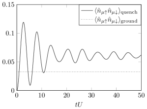
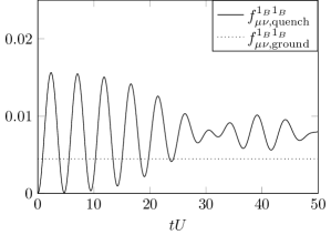
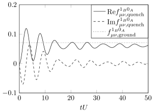
Figure 7: Time-dependence of the quantum depletion, the nearest-neighbor correlation function $f^{1_{B}0_{A}}_{\mu\nu}$, and the next-to-nearest-neighbor correlation function $f^{1_{B}1_{B}}_{\mu\nu}$ in three dimensions after a quench within the Mott phase according to $J/U=0\to 0.5$ in comparison to their ground-state values.

XIII Conclusions

In summary, we studied the quantum dynamics of the Bose and Fermi Hubbard model after a quench within the Mott phase. To this end, we employed a formal expansion into powers of $1/Z$ based on the hierarchy of correlations. In comparison to other approaches (as mentioned in the Introduction, for example), this method facilitates an iterative approximate analytical solution for the time dependence of the reduced density matrices and their ground state values. It is particularly suited for the strongly interacting regime in higher dimensions and can be applied to a general lattice structure $T_{\mu\nu}$ of arbitrary size. Since our method is based on an expansion into powers of the (small) control parameter $1/Z$, it provides a unique classification which effect occurs at which order in $1/Z$. This fact is also related to the somewhat disadvantageous features of our approach, for example the fact that the correct treatment of the soft spin modes and the late-time dynamics requires higher orders in $1/Z$. Furthermore, we cannot describe the transition between the Mott insulator and the metallic state in the Fermi-Hubbard model within our first-order approach.

As one application, we derive the spread of correlations and obtain an effective light-cone structure (via the saddle-point approximation). Furthermore, we found that the considered observables settle down to a quasi-equilibrium state after some time – but this state is not thermal. More precisely, the on-site density matrix settles down to a state which could be described by a thermal ensemble but the two-point correlations do not fit this thermal state.

Thus, real thermalization – if it occurs at all – requires much longer times scales. This seems to be a generic feature and has been discussed for bosonic KLA07 ; CFMSE08 ; FCMSE08 ; CDEO08 and fermionic systems U09 ; MK08 ; EKW10 ; MK09 ; MK10 ; SGJ10 ; EKW09 ; luttinger and is sometimes called “pre-thermalization” BBS03 ; BBW04 . This phenomenon can be visualized via the following intuitive picture: The excited state generated by the quench can be viewed as a highly coherent superposition of correlated quasi-particles. During the subsequent quantum evolution, these quasi-particles disperse and randomize their relative phases – which results in a quasi-stationary state. However, the quasi-particles still retain their initial spectrum (in energy and quasi-momentum), which could be approximately described by a generalized Gibbs ensemble (i.e., a momentum-dependent temperature). In this picture, thermalization requires the exchange of energy and momentum between these quasi-particles due to multiple collisions, which changes the one-particle spectrum and takes much longer. Ergo, one would expect a separation of time scales – i.e., first (quasi) equilibration and only much later thermalization – for many systems in condensed matter, where the above quasi-particle picture applies.

Within our $1/Z$ approach, the interaction between the quasi-particles (responsible for the exchange of energy and momentum by multiple collisions) correspond to higher orders in $1/Z$. Since they become relevant at time scales much longer than the initial dephasing time considered here, one would expect that it is possible to derive some sort of Boltzmann equation for these long time scales.

Appendix A Derivation of the hierarchy

In this Appendix, we derive the hierarchical set of equations for the correlation functions. The quantum evolution of the on-site density matrix can be derived by tracing von Neumann’s equation (6) over all lattice sites but $\mu$ and exploiting the invariance of the trace under cyclic permutations

$$i\partial_{t}\hat{\rho}_{\mu} = \frac{1}{Z}\,{\rm Tr}_{\not\mu}\left\{\sum_{\alpha,\beta\neq\mu}\mathcal{L}_{\alpha\beta}\hat{\rho}+\sum_{\alpha\neq\mu}\mathcal{L}^{S}_{\alpha\mu}\hat{\rho}\right\}$$ (96)

$$+\,{\rm Tr}_{\not\mu}\left\{\sum_{\alpha\neq\mu}\mathcal{L}_{\alpha}\hat{\rho}+\mathcal{L}_{\mu}\hat{\rho}\right\}$$

$$= \frac{1}{Z}\sum_{\alpha\neq\mu}\mathcal{L}^{S}_{\mu\alpha}\,{\rm Tr}_{\alpha}\{\hat{\rho}_{\mu\kappa}\}+\mathcal{L}_{\mu}\hat{\rho}_{\mu}\,.$$

Using the definition of the two-point correlations given in (8), we arrive at (9). Similarly, the differential equation for the two-particle density matrix can be deduced by tracing over all lattice sites but $\mu$ and $\nu$,

$$i\partial_{t}\hat{\rho}_{\mu\nu} = i\left(\partial_{t}\hat{\rho}_{\mu\nu}^{\mathrm{corr}}+\hat{\rho}_{\mu}\partial_{t}\hat{\rho}_{\nu}+\hat{\rho}_{\nu}\partial_{t}\hat{\rho}_{\mu}\right)$$ (97)

$$= \frac{1}{Z}\sum_{\alpha\neq\mu\nu}\left(\,{\rm Tr}_{\alpha}\left\{\mathcal{L}_{\mu\kappa}^{S}\hat{\rho}_{\mu\nu\alpha}\right\}+\,{\rm Tr}_{\alpha}\left\{\mathcal{L}_{\kappa\nu}^{S}\hat{\rho}_{\mu\nu\alpha}\right\}\right)$$

$$+\frac{1}{Z}\mathcal{L}_{\mu\nu}^{S}\hat{\rho}_{\mu\nu}+\mathcal{L}_{\mu}\hat{\rho}_{\mu\nu}+\mathcal{L}_{\nu}\hat{\rho}_{\mu\nu}\,.$$

With the definitions (8) and the time-evolution for the single-site density matrix (96), we find for the two-point correlation functions (10). The equations (9) and (10) preserve the hierarchy in time if initially $\hat{\rho}_{\mu}=\mathcal{O}(Z^{0})$ and $\hat{\rho}_{\mu\nu}^{\mathrm{corr}}=\mathcal{O}(1/Z)$ holds. In order to derive the full hierarchy, we define the generating functional

$${\cal F}(\hat{\alpha})={\cal F}(\{\hat{\alpha}_{\mu}\})=\ln\left[\,{\rm Tr}\left\{\hat{\rho}\bigotimes_{\mu}(\mathbf{1}_{\mu}+\hat{\alpha}_{\mu})\right\}\right]\,,$$ (98)

where $\hat{\rho}$ is the density matrix of the full lattice and

$$\hat{\alpha}_{\mu}=\sum_{m,n}\alpha_{\mu}^{m,n}|m\rangle_{\mu}\langle n|$$ (99)

are arbitrary operators acting on the Hilbert spaces associated to the lattice sites $\mu$ with the local basis $\{\left|n\right>_{\mu}\}$. The role of this functional is to generate all correlated density matrices via the derivatives with respect to these operators $\hat{\alpha}_{\mu}$ which are defined via

$$\frac{\partial{\cal F(\{\alpha\})}}{{\partial\hat{\alpha}_{\mu}}} = \sum_{m,n}|n\rangle_{\mu}\langle m|\,\frac{\partial\cal F(\{\alpha\})}{\partial\alpha^{m,n}_{\mu}}$$ (100)

$$= \sum_{m,n}|n\rangle_{\mu}\langle m|\,\frac{\partial{\cal F}(\{\alpha\})}{\partial\,{{}_{\mu}\!\left<m\right|}\hat{\alpha}_{\mu}\left|n\right>_{\mu}}\,.$$

If we consider an ensemble ${\cal S}=\{\mu_{1},\dots,\mu_{\ell}\}$ of $\ell$ different lattice sites $\mu_{1}\not=\dots\not=\mu_{\ell}$, we obtain the correlation operators via

$$\hat{\rho}^{\rm corr}_{\cal S}=\left.\frac{\partial}{\partial\hat{\alpha}_{\mu_{1}}}\frac{\partial}{\partial\hat{\alpha}_{\mu_{2}}}\dots\frac{\partial}{\partial\hat{\alpha}_{\mu_{\ell}}}{\cal F}(\hat{\alpha})\right|_{\hat{\alpha}=0}\,.$$ (101)

These operators are related to the corresponding reduced density matrix operator $\rho_{\cal S}$ through the relation

$$\hat{\rho}_{\cal S}=\hat{\rho}_{\mu_{1}\dots\mu_{\ell}}=\sum_{\cup_{i}{\cal P}_{i}={\cal S}}\prod_{i}\hat{\rho}^{\rm corr}_{{\cal P}_{i}}$$ (102)

where the sum runs over all possible segmentations of the subset ${\cal S}$ into partitions ${\cal P}_{i}$ starting from the whole subset ${\cal P}={\cal S}$ and ranging to single lattice sites ${\cal P}_{i}=\{\mu\}$ where $\hat{\rho}^{\rm corr}_{{\cal P}_{i}=\{\mu\}}=\hat{\rho}_{\mu}$ is understood. For two and three lattice sites, the above equation reproduces Eq. (8).

Our derivation is based on the following scaling hierarchy of correlations:

$$\hat{\rho}_{\cal S}^{\rm c}=\,{\cal O}\left(Z^{1-|\cal S|}\right)$$ (103)

where $|\cal S|$ is the number $\ell$ of lattice sites in the set $\cal S$. From the Liouville equation (6), the temporal evolution of ${\cal F}$ is given by

$$i\partial_{t}{\cal F}(\hat{\alpha})=\sum_{\mu}\,{\rm Tr}_{\mu}\left\{\hat{\alpha}_{\mu}\,\widehat{\cal L}_{\mu}\frac{\partial{\cal F}}{\partial\hat{\alpha}_{\mu}}\right\}+\frac{1}{Z}\sum_{\mu,\nu}\,{\rm Tr}_{\mu\nu}\left\{(\hat{\alpha}_{\mu}+\hat{\alpha}_{\nu}+\hat{\alpha}_{\mu}\hat{\alpha}_{\nu})\,\widehat{\cal L}_{\mu\nu}\left(\frac{\partial^{2}{\cal F}}{\partial\hat{\alpha}_{\mu}\partial\hat{\alpha}_{\nu}}+\frac{\partial{\cal F}}{\partial\hat{\alpha}_{\mu}}\frac{\partial{\cal F}}{\partial\hat{\alpha}_{\nu}}\right)\right\}\,.$$ (104)

By taking successive derivatives and using the generalized Leibniz rule

$$\frac{\partial}{\partial\hat{\alpha}_{\mu_{1}}}\frac{\partial}{\partial\hat{\alpha}_{\mu_{2}}}\dots\frac{\partial}{\partial\hat{\alpha}_{\mu_{\ell}}}\left[{\cal F}(\hat{\alpha})\right]^{2}=\sum_{{\cal P}\subseteq{\cal S}}^{{\cal P}\cup\bar{\cal P}={\cal S}}\left[\left(\prod_{\mu_{i}\in{\cal P}}\frac{\partial}{\partial\hat{\alpha}_{\mu_{i}}}\right){\cal F}(\hat{\alpha})\right]\left[\left(\prod_{\mu_{j}\in\bar{\cal P}}\frac{\partial}{\partial\hat{\alpha}_{\mu_{j}}}\right){\cal F}(\hat{\alpha})\right]\,,$$ (105)

as well as the the property

$$\frac{\partial^{2}{\cal F}(\hat{\alpha})}{\partial\hat{\alpha}_{\mu}^{2}}=\frac{\partial}{\partial\hat{\alpha}_{\mu}}\frac{\partial}{\partial\hat{\alpha}_{\mu}}{\cal F}(\hat{\alpha})=-\frac{\partial{\cal F}(\hat{\alpha})}{\partial\hat{\alpha}_{\mu}}\frac{\partial{\cal F}(\hat{\alpha})}{\partial\hat{\alpha}_{\mu}}=-\left(\frac{\partial{\cal F}(\hat{\alpha})}{\partial\hat{\alpha}_{\mu}}\right)^{2}\,,$$ (106)

we establish the following set of equations for the correlated density matrices:

$$i\partial_{t}\hat{\rho}^{\rm corr}_{\cal S} = \frac{1}{Z}\sum_{\mu,\nu\in{\cal S}}\sum_{{\cal P}\subseteq{\cal S}\setminus\{\mu,\nu\}}^{{\cal P}\cup\bar{\cal P}={\cal S}\setminus\{\mu,\nu\}}\Bigg{\{}\,\widehat{\cal L}_{\mu\nu}\,\hat{\rho}^{\rm corr}_{\{\mu\}\cup{\cal P}}\,\hat{\rho}^{\rm corr}_{\{\nu\}\cup\bar{\cal P}}-\,{\rm Tr}_{\nu}\Bigg{[}\,\widehat{\cal L}^{S}_{\mu\nu}(\hat{\rho}^{\rm corr}_{\{\mu,\nu\}\cup\bar{\cal P}}+\sum_{{\cal Q}\subseteq\bar{\cal P}}^{{\cal Q}\cup\bar{\cal Q}=\bar{\cal P}}\hat{\rho}^{\rm corr}_{\{\mu\}\cup{\cal Q}}\,\hat{\rho}^{\rm corr}_{\{\nu\}\cup\bar{\cal Q}})\Bigg{]}\hat{\rho}^{\rm corr}_{\{\nu\}\cup{\cal P}}\Bigg{\}}$$ (107)

$$+\sum_{\mu\in{\cal S}}\,\widehat{\cal L}_{\mu}\hat{\rho}^{\rm corr}_{\cal S}+\frac{1}{Z}\sum_{\mu,\nu\in{\cal S}}\,\widehat{\cal L}_{\mu\nu}\,\hat{\rho}^{\rm corr}_{\cal S}+\frac{1}{Z}\sum_{\kappa\notin{\cal S}}\sum_{\mu\in{\cal S}}\,{\rm Tr}_{\kappa}\Bigg{[}\,\widehat{\cal L}^{S}_{\mu\kappa}\hat{\rho}^{\rm corr}_{{\cal S}\cup{\kappa}}+\sum_{{\cal P}\subseteq{\cal S}\setminus\{\mu\}}^{{\cal P}\cup\bar{\cal P}={\cal S}\setminus\{\mu\}}\,\widehat{\cal L}^{S}_{\mu\kappa}\hat{\rho}^{\rm corr}_{\{\mu\}\cup{\cal P}}\,\hat{\rho}^{\rm corr}_{\{\kappa\}\cup\bar{\cal P}}\Bigg{]}\,.$$

For $\ell=1$ and $\ell=2$ we recover the equations (9) and (10). A careful inspection of this set of equations shows that the hierarchy in (103) is preserved in time: Imposing the scaling $\hat{\rho}^{\rm corr}_{\cal S}=\,{\cal O}(Z^{1-|\cal S|})$ on the r.h.s. of the above equation, we find that the time derivative on the l.h.s. does also satisfy the hierarchy (103). Therefore, inserting (103) into (107) and taking the limit $Z\to\infty$, we obtain the leading-order contributions

$$i\partial_{t}\hat{\rho}^{\rm corr}_{\cal S} = \frac{1}{Z}\sum_{\mu,\nu\in{\cal S}}\sum_{{\cal P}\subseteq{\cal S}\setminus\{\mu,\nu\}}^{{\cal P}\cup\bar{\cal P}={\cal S}\setminus\{\mu,\nu\}}\Bigg{\{}\,\widehat{\cal L}_{\mu\nu}\,\hat{\rho}^{\rm corr}_{\{\mu\}\cup{\cal P}}\,\hat{\rho}^{\rm corr}_{\{\nu\}\cup\bar{\cal P}}-\,{\rm Tr}_{\nu}\Bigg{[}\,\widehat{\cal L}^{S}_{\mu\nu}\sum_{{\cal Q}\subseteq\bar{\cal P}}^{{\cal Q}\cup\bar{\cal Q}=\bar{\cal P}}\hat{\rho}^{\rm corr}_{\{\mu\}\cup{\cal Q}}\,\hat{\rho}^{\rm corr}_{\{\nu\}\cup\bar{\cal Q}}\Bigg{]}\hat{\rho}^{\rm corr}_{\{\nu\}\cup{\cal P}}\Bigg{\}}$$ (108)

$$+\sum_{\mu\in{\cal S}}\,\widehat{\cal L}_{\mu}\hat{\rho}^{\rm corr}_{\cal S}+\frac{1}{Z}\sum_{\kappa\notin{\cal S}}\sum_{\mu\in{\cal S}}\,{\rm Tr}_{\kappa}\Bigg{[}\sum_{{\cal P}\subseteq{\cal S}\setminus\{\mu\}}^{{\cal P}\cup\bar{\cal P}={\cal S}\setminus\{\mu\}}\,\widehat{\cal L}^{S}_{\mu\kappa}\hat{\rho}^{\rm corr}_{\{\mu\}\cup{\cal P}}\,\hat{\rho}^{\rm corr}_{\{\kappa\}\cup\bar{\cal P}}\Bigg{]}+\,{\cal O}(Z^{-|\cal S|})\,.$$

For $\ell=1$ and $\ell=2$, we recover equations (11) and (12).

In contrast to the exact expression (107), the approximated leading-order equations (108) form a closed set. The exact time evolution (107) of the $|\cal S|$-point correlator $\partial_{t}\hat{\rho}^{\rm corr}_{\cal S}$ also depends on the higher-order correlation term $\hat{\rho}^{\rm corr}_{{\cal S}\cup{\kappa}}$ involving $|{\cal S}|+1$ points. The approximated expression (108), on the other hand, only contains correlators of the same or lower rank. This facilitates the iterative solution of the problem sketched in Section III. First one solves the zeroth-order equation (11) for $\hat{\rho}_{\mu}^{0}$. Inserting this result $\hat{\rho}_{\mu}^{0}$ into the first-order (in $1/Z$) equation (12) for $\hat{\rho}_{\mu\nu}^{\rm corr}$, we obtain a first-order result for $\hat{\rho}_{\mu\nu}^{\rm corr}$. This first-order result for $\hat{\rho}_{\mu\nu}^{\rm corr}$ can then be inserted into the equation for $\hat{\rho}_{\mu\nu\lambda}^{\rm corr}$ which is of second order $1/Z^{2}$. Furthermore, we may use the first-order result for $\hat{\rho}_{\mu\nu}^{\rm corr}$ in order to obtain a better approximation for the one-point density matrix $\hat{\rho}_{\mu}^{1}$ which is valid to first order in $1/Z$ and contains the quantum depletion etc. Repeating this iteration, we may successively “climb up” to higher and higher orders in $1/Z$.

References

• (1) J. M. Deutsch, Phys. Rev. A 43, 2046 (1991).
• (2) M. Srednicki, Phys. Rev. E 50, 888 (1994).
• (3) J. Berges, S. Borsányi, and J. Serreaua, Nucl. Phys. B 660, 51 (2003).
• (4) J. Berges, S. Borsányi, and C. Wetterich, Phys. Rev. Lett. 93, 142002 (2004).
• (5) P. Calabrese and J. Cardy, Phys. Rev. Lett. 96, 136801 (2006).
• (6) P. Calabrese and J. Cardy, J. Stat. Mech. P06008 (2007).
• (7) M. Rigol, V. Dunjko, V. Yurovsky, and M. Olshanii, Phys. Rev. Lett. 98, 050405 (2007).
• (8) M. Rigol, V. Dunjko, and M. Olshanii, Nature (London) 452, 854 (2008).
• (9) M. Eckstein, A. Hackl, S. Kehrein, M. Kollar, M. Moeckel, P. Werner, and F. A. Wolf, Eur. Phys. J. Spec. Top. 180, 217 (2009).
• (10) M. Moeckel and S. Kehrein, Ann. Phys. 324, 2146 (2009).
• (11) M. A. Cazalilla and M. Rigol, New J. Phys. 12, 055006 (2010).
• (12) A. Polkovnikov, K. Sengupta, A. Silva, and M. Vengalattore, Rev. Mod. Phys. 83, 863 (2011).
• (13) M. Kollar, F. A. Wolf, and M. Eckstein, Phys. Rev. B 84, 054304 (2011).
• (14) C. Gogolin, M. P. Müller, and J. Eisert, Phys. Rev. Lett. 106, 040401 (2011).
• (15) T. Kitagawa, A. Imambekov, J. Schmiedmayer, and E. Demler, New J. Phys. 13, 073018 (2011).
• (16) M. C. Ba$\tilde{\mathrm{n}}$uls, J. I. Cirac, and M. B. Hastings, Phys. Rev. Lett. 106, 050405 (2011).
• (17) M. Rigol and M. Srednicki, Phys. Rev. Lett. 108, 110601 (2012).
• (18) M. Rigol, in Quantum Gases: Finite Temperature and Non-Equilibrium Dynamics (Vol. 1 Cold Atoms Series), N. P. Proukakis, S. A. Gardiner, M. J. Davis, and M. H. Szymanska, eds. (Imperial College Press, London 2013).
• (19) D. Jaksch and P. Zoller, Annals of Physics 315, 52 (2005).
• (20) O. Morsch and M. Oberthaler, Rev. Mod. Phys. 78, 179 (2006).
• (21) M. Lewenstein, A. Sanpera, V. Ahufinger, B. Damski, A. Sen (De), and U. Sen, Adv. Phys. 56, 243 (2007).
• (22) I. Bloch, J. Dalibard, and W. Zwerger, Rev. Mod. Phys. 80, 885 (2008).
• (23) V. I. Yukalov, Laser Phys. 19, 1 (2009).
• (24) M. Lewenstein, A. Sanpera, and V. Ahufinger, Ultracold Atoms in Optical Lattices: Simulating quantum many-body systems (Oxford University Press 2012).
• (25) C. Kollath, A. M. Läuchli, E. Altman, Phys. Rev. Lett. 98, 180601 (2007).
• (26) G. Biroli, C. Kollath, and A. M. Läuchli, Phys. Rev. Lett. 105, 250401 (2010).
• (27) G. Roux, Phys. Rev. A 79, 021608 (2009).
• (28) G. Roux, Phys.  Rev. A 81, 053604 (2010).
• (29) M. Cramer, C. M. Dawson, J. Eisert, and T. J. Osborne, Phys. Rev. Lett. 100, 030602 (2008).
• (30) M. Cramer , A. Flesch, I. P. McCulloch, U. Schollwöck, and J. Eisert, Phys. Rev. Lett. 101, 063001 (2008).
• (31) A. Flesch, M. Cramer, I. P.  McCulloch, U. Schollwöck, and J. Eisert, Phys. Rev. A 78, 033608 (2008).
• (32) A. M. Läuchli and C. Kollath, J. Stat. Mech.: Theory and Experiment, P05018 (2008).
• (33) J.-S. Bernier, G. Roux, and C. Kollath, Phys. Rev. Lett. 106 200601 (2011).
• (34) J-S. Bernier, D. Poletti, P. Barmettler, G. Roux, and C. Kollath, Phys. Rev. A 85, 033641 (2012).
• (35) P. Barmettler, D. Poletti, M. Cheneau, and C. Kollath, Phys. Rev. A 85, 053625 (2012).
• (36) M. Greiner, O. Mandel, T. W. Hänsch and I. Bloch, Nature (London) 419, 51 (2002).
• (37) T. Kinoshita, T. Wenger, and D. Weiss, Nature (London) 440, 900 (2006).
• (38) S. Trotzky, Y. Chen, A. Flesch, I. P. McCulloch, U. Schollwck, J. Eisert, and I. Bloch, Nature Physics 8, 325 (2012).
• (39) M. Cheneau, P. Barmettler, D. Poletti, M. Endres, P. Schauß, T. Fukuhara, C. Gross, I. Bloch, C. Kollath, and S. Kuhr, Nature (London) 481, 484 (2012).
• (40) M. Gring, M. Kuhnert, T. Langen, T. Kitagawa, B. Rauer, M. Schreitl, I. Mazets, D. Adu Smith, E. Demler, J. Schmiedmayer, Science 337, 1318 (2012).
• (41) R. Schützhold, M. Uhlmann, Y. Xu, and U. R. Fischer, Phys. Rev. Lett. 97, 200601 (2006).
• (42) U. R. Fischer, R. Schützhold, and M. Uhlmann, Phys. Rev. A 77, 043615 (2008).
• (43) S. S. Natu and E. J. Mueller, Phys.  Rev. A 87, 053607 (2013);
• (44) S. S. Natu and E.J. Mueller, Phys.  Rev. A 87, 063616 (2013).
• (45) S. S. Natu, K. R. A. Hazzard, and E. J. Mueller, Phys.  Rev.  Lett. 106, 125301 (2011).
• (46) B. Sciolla and G. Biroli, J. Stat. Mech.: Theory and Experiment, P11003 (2008).
• (47) B. Sciolla and G. Biroli, Phys.  Rev.  Lett. 105, 220401 (2010).
• (48) J. D. Sau, B. Wang, and S. Das Sarma, Phys.  Rev.  A 85, 013644 (2012).
• (49) D. Chen, M. White, C. Borries, and B. DeMarco, Phys. Rev. Lett. 106, 235304 (2011).
• (50) M. Kollar and M. Eckstein, Phys. Rev. A 78, 013626 (2008).
• (51) S. A. Hamerla and G. S. Uhrig, Phys. Rev. B 87, 064304 (2013).
• (52) F. Goth and F. F. Assaad, Phys. Rev. B 85, 085129 (2012).
• (53) M. Eckstein, M. Kollar, and P. Werner, Phys. Rev. Lett. 103, 056403 (2009).
• (54) M. Eckstein, M. Kollar, and P. Werner, Phys. Rev. B 81, 115131 (2010).
• (55) P. Anders, E.  Gull, L. Pollet, M.  Troyer, and P. Werner, Phys. Rev. Lett. 105, 096402 (2010);
• (56) P. Anders, E. Gull, L. Pollet, M. Troyer, and P. Werner, New J. Phys. 13, 075013 (2011).
• (57) P. Werner, N. Tsuji, and M. Eckstein, Phys. Rev. B 86, 205101 (2012).
• (58) M. Schiró and M. Fabrizio, Phys. Rev. Lett. 105, 076401 (2010).
• (59) M. Schiró and M. Fabrizio, Phys. Rev. B 83, 165105 (2011).
• (60) M. Sandri, M. Schiró, and M. Fabrizio, Phys.  Rev. B 86, 075122 (2012).
• (61) M. Moeckel and S. Kehrein, Phys. Rev. Lett. 100, 175702 (2008).
• (62) M. Moeckel and S. Kehrein, New J. Phys. 12, 055016 (2010).
• (63) N. Strohmaier, D. Greif, R. Jördens, L. Tarruell, H. Moritz, and T. Esslinger, Phys. Rev. Lett. 104, 080401 (2010).
• (64) A. Hubener, M. Snoek, and W. Hofstetter, Phys. Rev. B 80, 245109 (2009).
• (65) M. P. A. Fisher, P. B. Weichman, G. Grinstein, and D. S. Fisher, Phys. Rev. B 40, 546 (1989).
• (66) D. Jaksch, C. Bruder, J. I. Cirac, C. W. Gardiner, and P. Zoller, Phys. Rev. Lett. 81, 3108 (1998).
• (67) W. Zwerger, J. Opt. B: Quantum Semiclass. Opt. 5, S9 (2003).
• (68) S. Sachdev, Quantum phase transitions, (Cambridge University Press, Cambridge, England, 2001).
• (69) Note that one should be careful what type of correlations are considered. For example, the Mott state is often referred to as correlated because the many-body wave-function $\Psi(\mbox{\boldmath$r$}_{1},\mbox{\boldmath$r$}_{2},\dots)$ cannot be written as a symmetrized product $\Psi(\mbox{\boldmath$r$}_{1},\mbox{\boldmath$r$}_{2},\dots)\neq{\cal S}[\psi_{1}(\mbox{\boldmath$r$}_{1})\psi_{2}(\mbox{\boldmath$r$}_{2})\dots].$ This corresponds to correlations between the particle positions such as $\mbox{\boldmath$r$}_{1}$ and $\mbox{\boldmath$r$}_{2}$, i.e., if one particle $\mbox{\boldmath$r$}_{1}$ is at the lattice site $\mu$, the other particle $\mbox{\boldmath$r$}_{2}$ is very likely not at the same site due to the strong repulsion $U$. In this paper, we do not consider this type of correlations (e.g., between $\mbox{\boldmath$r$}_{1}$ and $\mbox{\boldmath$r$}_{2}$) but instead the correlations between lattice sites $\mu$ and $\nu$.
• (70) I. Bloch, Nature Physics, 1, 23 (2005).
• (71) C. Sias, A. Zenesini, H. Lignier, S. Wimberger, D. Ciampini, O. Morsch, and E. Arimondo, Phys. Rev. Lett. 98, 120403 (2007).
• (72) M. Raizen, C. Salomon, and Q. Niu, Physics Today, 50, 30 (1997).
• (73) M. Greiner, O. Mandel, T. Esslinger, T. W. Hänsch, and I. Bloch, Nature (London) 415, 39 (2002).
• (74) J. K. Freericks and H. Monien, Europhys. Lett. 26 545, (1994).
• (75) J. K. Freericks and H. Monien, Phys. Rev. B 53, 2691 (1996).
• (76) B. Damski and J. Zakrzewski Phys. Rev. A 74, 043609 (2006).
• (77) J. K. Freericks, H. R. Krishnamurthy, Y. Kato, N. Kawashima, and N. Trivedi, Phys. Rev. A 79, 053631 (2009).
• (78) Y. Li, M. R. Bakhtiari, L. He, and W. Hofstetter, Phys. Rev. B 84, 144411 (2011).
• (79) Y. Li, M. R. Bakhtiari, L. He, and W. Hofstetter, Phys. Rev. A 85, 023624 (2012).
• (80) M. C. Gutzwiller, Phys. Rev. Lett. 10, 159 (1963).
• (81) D. S. Rokhsar and B. G. Kotliar, Phys. Rev. B 44, 10328 (1991).
• (82) M. Christandl, R. Koenig, G. Mitchison, and R. Renner, Comm. Math. Phys. 273, 473 (2007).
• (83) R. Kubo, J. Phys. Soc. Japan 17, 1100 (1962).
• (84) R. Balescu, Equilibrium and Nonequilibrium Statistical Mechanics (Wiley, New York, 1975).
• (85) H. R. Krishnamurthy, C. Jayaprakash, S. Sarker, and W. Wenzel, Phys. Rev. Lett. 64, 950 (1990).
• (86) F. Queisser, P. Navez, and R. Schützhold, Phys. Rev. A 85, 033625 (2012).
• (87) K. Krutitsky and P. Navez, Phys. Rev. A 84, 033602 (2011).
• (88) K. Sengupta and N. Dupuis, Phys. Rev. A 71, 033629 (2005).
• (89) S. D. Huber, E. Altman, H. P. Büchler, and G. Blatter, Phys. Rev. B 75, 085106 (2007).
• (90) M. Snoek, Europhys. Lett. 95, 30006 (2011).
• (91) P. Navez and R. Schützhold, Phys. Rev. A 82, 063603 (2010).
• (92) Note that, in contrast to the $\,{\cal O}(J)$-terms in Eqs. (49) and (50), the existence of the $\,{\cal O}(J^{2})$-terms in Eqs. (51) and (52) depends on the lattice structure. In the case of a hyper-cubic lattice with rectangular tunneling to nearest neighbors only, for example, the sum over $\kappa$ in Eqs. (51) and (52) contains at most two non-vanishing terms and thus the correlators in (51) and (52) are of order $1/Z^{2}$. For a hyper-cubic lattice with additional diagonal tunneling, on the other hand, the $\kappa$-sum can involve $\,{\cal O}(Z)$ non-zero contributions, which yields correlators (51) and (52) of order $1/Z$.
• (93) F. Queisser et al, manuscript in preparation.
• (94) J. Hubbard, Proc. R. Soc. Lond. A 276, 238 (1963).
• (95) F. H. L. Essler, H. Frahm, F. Göhmann, A. Klümper, and V. E. Korepin, The One-Dimensional Hubbard Model, Cambridge University Press (2005).
• (96) E. Fradkin, Field Theories Of Condensed Matter Systems, Addison-Wesley (1991).
• (97) W. Metzner and D. Vollhardt, Phys. Rev. Lett. 62, 324 (1989).
• (98) P. Fazekas, Lecture Notes On electron Correlation and Magnetism, World Scientific (1999).
• (99) A. Auerbach, Interacting Electrons And Quantum Magnetism, Springer (1994).
• (100) W. Langer, M. Plischke, and D. Mattis, Phys. Rev. Lett. 23, 1448 (1969).
• (101) D. Baeriswyl, D. Eichenberger, and M. Menteshashvili, New J. Phys. 11, 075010 (2009).
• (102) A. Georges, G. Kotliar, W. Krauth, and M. J. Rozenberg, Rev. Mod. Phys. 68, 13 (1996).
• (103) G. S. Uhrig, Phys. Rev. A 80, 061602 (2009).
• (104) A. Iucci and M. A. Cazalilla, Phys. Rev. A 80, 063619 (2009).