Rigorous numerical verification of uniqueness and smoothness in a surface growth model

Abstract

Based on numerical data and a-posteriori analysis we verify rigorously the uniqueness and smoothness of global solutions to a scalar surface growth model with striking similarities to the 3D Navier–Stokes equations, for certain initial data for which analytical approaches fail. The key point is the derivation of a scalar ODE controlling the norm of the solution, whose coefficients depend on the numerical data. Instead of solving this ODE explicitly, we explore three different numerical methods that provide rigorous upper bounds for its solution.

1 Introduction

We consider the following surface growth equation for the height $u(t,x)\in\mathbb{R}$ at time $t>0$ over a point $x\in[0,2\pi]$

$$u_{t}=-u_{xxxx}-({u_{x}}^{2})_{xx}\qquad x\in[0,2\pi],\;t\in[0,T]$$ (1)

with periodic boundary conditions and subject to a moving frame, which yields the zero-average condition $\int_{0}^{2\pi}u(x,t)\;\mathrm{d}x=0$.

This equation, usually with additional noise terms, was introduced as a phenomenological model for the growth of amorphous surfaces [21, 18], and was also used to describe sputtering processes [6]; see [3] for a detailed list of references. Based on the papers [4, 7, 19] which develop the theory of ‘numerical verification of regularity’ for the 3D Navier–Stokes equations, our aim here is to establish and implement numerical algorithms to prove rigorously global existence and uniqueness of solutions of (1).

Despite being scalar the equation has surprising similarities to 3D Navier–Stokes equations [1, 2, 3]. It allows for a global energy estimate in $L^{2}$ and uniqueness of smooth local solutions for initial conditions in a critical Besov-type space that contains $C^{0}$ and $H^{1/2}$, see [3] (similar results for the 3D Navier–Stokes equations can be found in [9]). Here we focus on the one-dimensional model, since in this case more efficient numerical methods are available, and the calculations would be significantly slower in higher dimension. Moreover, for the two-dimensional case the situation of energy estimates seems even worse, as global existence could only be established in $H^{-1}$ using the non-standard energy $\int_{0}^{2\pi}{\rm e}^{u(x)}\,{\rm d}x$, see [22] for details. Nevertheless, we believe that it should be possible to treat the 2D case using similar methods, but the analysis becomes more delicate since in two dimensions $H^{1}$ is the critical space (see [2, 3]).

Rigorous methods for proving numerically the existence of solutions for PDEs are a recent and active research field. In addition to the approach taken here there are methods based on topological arguments like the Conley index, see [11, 8, 23], for example. For solutions of elliptic PDEs there are methods using Brouwer’s fixed-point theorem, as discussed in the review article [17] and the references therein.

Our approach is based on [4] and similar to the method proposed in [14]. The key point is the derivation of a scalar ODE for the $H^{1}$-norm of the difference of an arbitrary approximation, that satisfies the boundary conditions, to the solution. The coefficients of this ODE depend only on the numerical data (or any other approximation used). As long as the solution of the ODE stays finite, one can rely on the continuation property of unique local solutions, and thus have a smooth unique solution up to a blowup time of the ODE. A similar approach using an integral equation based on the mild formulation was proposed in [12, 13].

In order to establish a bound on the blow-up time for the ODE, one can either proceed analytically or numerically. We propose two analytical methods: one, based on the standard Gronwall Lemma, enforces a ‘small data’ hypothesis and adds little to standard analytical existence proofs. The second is based on an explicit analytical upper bound to the ODE solution. A variant of this, a hybrid method in which one applies an analytical upper bound on a succession of small intervals of length $h>0$ to the numerical solution and then restarts the argument, appears the most promising, and a formal calculation indicates that the upper bound from the third method in the limit of step-size to zero converges to the solution of the ODE.

In order to derive the ODE for the $H^{1}$-error, we use standard a-priori estimates. While the stability of the linear term $-u_{xxxx}$ means that these ‘worst case’ estimates are still sufficient, an interesting alternative approach in a slightly different context is proposed in [15, 16], where the spectrum of the linearized operator (here $Lv=-v_{xxxx}+(v_{x}\varphi_{x})_{xx}$, where $\varphi$ is some given numerical data) is analysed with a rigorous numerical method, which in the case of an unstable linear operator yields substantially better results, at the price of a significantly higher computational time. This will be the subject of future research.

The paper is organized as follows. In Section 2 we establish the a-priori estimates for the $H^{1}$-error between solutions and the numerical data, which in the end gives an ODE depending on the numerical data only. Section 3 provides the ODE estimates necessary for our three methods, while Section 4 states the main results. In the final Section 5, we compare our methods using numerical experiments.

2 A-priori analysis

In this section we establish upper bounds for the $H^{1}$-norm of the error

$$d(x,t):=u(x,t)-\varphi(x,t),$$

where $u$ is a solution to our surface growth equation (1) and $\varphi$ is any arbitrary, but sufficiently smooth approximation, that satisfies the boundary conditions. Since we know $\varphi$, if we can control the $H^{1}$ norm of $d$ then we control the $H^{1}$ norm of $u$.

For the following estimates and results, we define the $H^{p}$-norm, $p\geq 1$, of a function $u$ by

$$\|u\|_{H^{p}}:=\left\|\partial_{x}^{p}u\right\|_{L^{2}},$$

which is equivalent to the standard $H^{p}$-norm as we only consider functions with vanishing mean, i.e. $\int_{0}^{2\pi}u(x,t)\;\mathrm{d}x=0$. Note that in this setting Agmon’s inequality

$$\|u\|_{L^{\infty}}\leq\|u\|_{L^{2}}^{1/2}\|u_{x}\|_{L^{2}}^{1/2}$$ (2)

holds with optimal constant $1$, which follows using the Fourier expansion.

A very important property of the surface growth equation (1) is the existence of local solutions, which are smooth in space and time. This result is given by the following theorem from [2] (Theorem 3.1).

Theorem 1.

Let $u_{0}\in H^{1}$, then there exists a time $\tau(u_{0})>0$ such that there is a unique solution $u\in C^{0}([0,\tau(u_{0})),H^{1})$ satisfying

1. if $\tau(u_{0})<\infty$, then $\limsup\limits_{t\rightarrow\infty}\|u(t)\|_{H^{1}}=\infty$.

2. $u$ is $C^{\infty}$ in both, space and time, for all $(t,x)\in(0,\tau(u_{0}))\times[0,2\pi]$.

Note that the theorem implies that lack of blowup in $H^{1}$ is sufficient to ensure that the solution exists for all time and is smooth. In particular, all of the manipulations we make in what follows are valid until the blowup time.

Throughout the rest of the paper we consider the solutions with initial data in $H^{1}$ whose existence is guaranteed by Theorem 1, and approximations $\varphi\in H^{4}_{\text{per}}$ in space and $H^{1}$ in time.

2.1 Energy estimate

In this section we prove the key estimate (2.1) on which the theorems of the following sections are based.

If we use the surface growth equation (1) to find the evolution of $d(x,t)$ and defining the residual of the approximation $\varphi$ by

$$\operatorname{Res}:=\varphi_{t}+\varphi_{xxxx}+({\varphi_{x}}^{2})_{xx},$$

then we have

$$d_{t}=-d_{xxxx}-({u_{x}}^{2})_{xx}+({\varphi_{x}}^{2})_{xx}-\operatorname{Res}.$$

By replacing $u$ with $d+\varphi$ we obtain

$$d_{t}=-d_{xxxx}-({d_{x}}^{2})_{xx}-2(d_{x}\varphi_{x})_{xx}-\operatorname{Res}.$$

For the $H^{1}$-norm we have

$$\frac{1}{2}\partial_{t}\|d_{x}\|^{2}= \underbrace{\left\langle d_{xx},d_{xxxx}\right\rangle}_{\mathrm{A}}+\underbrace{2\langle d_{xx},\left(d_{x}\varphi_{x}\right)_{xx}\rangle}_{\mathrm{B}}+\underbrace{\langle d_{xx},({d_{x}}^{2})_{xx}\rangle}_{\mathrm{C}}+\underbrace{\langle d_{xx},\operatorname{Res}\rangle}_{\mathrm{D}},$$

where $\langle\cdot,\cdot\rangle$ is the $L^{2}$ scalar product. Now consider these terms separately. Integrating by parts we obtain $\mathrm{A}=-\left\|d_{xxx}\right\|_{L^{2}}^{2}$. Secondly,

$$\mathrm{B}=-2\int_{0}^{2\pi}d_{xxx}(d_{x}\varphi_{x})_{x}\,\mathrm{d}x=\;\int_{0}^{2\pi}\left(d_{xx}\right)^{2}\varphi_{xx}\;\mathrm{d}x-2\int_{0}^{2\pi}d_{xxx}d_{x}\varphi_{xx}\;\mathrm{d}x\;$$

and so

$$|\mathrm{B}|\leq \;\left\|d_{xx}\right\|_{L^{2}}^{2}\left\|\varphi_{xx}\right\|_{L^{\infty}}+2\left\|d_{xxx}\right\|_{L^{2}}\left\|d_{x}\right\|_{L^{2}}\left\|\varphi_{xx}\right\|_{L^{\infty}}$$

$$\leq \;3\left\|d_{xxx}\right\|_{L^{2}}\left\|d_{x}\right\|_{L^{2}}\left\|\varphi_{xx}\right\|_{L^{\infty}}$$

$$\leq \;\frac{1}{4}\left\|d_{xxx}\right\|_{L^{2}}^{2}+9\left\|d_{x}\right\|_{L^{2}}^{2}\left\|\varphi_{xx}\right\|_{L^{\infty}}^{2},$$

using interpolation and Young’s inequality. For $C$ we have

$$\mathrm{C}=-\int_{0}^{2\pi}({d_{x}}^{2})_{x}d_{xxx}\;\mathrm{d}x=-2\int_{0}^{2\pi}d_{x}d_{xx}d_{xxx}\;\mathrm{d}x,$$

hence using Agmon’s inequality (2), interpolation, and Young’s inequality,

$$|\mathrm{C}|\leq \;2\left\|d_{x}\right\|_{L^{2}}\left\|d_{xx}\right\|_{L^{\infty}}\left\|d_{xxx}\right\|_{L^{2}}$$

$$\leq \;2\left\|d_{x}\right\|_{L^{2}}\left\|d_{xx}\right\|_{L^{2}}^{\frac{1}{2}}\left\|d_{xxx}\right\|_{L^{2}}^{\frac{3}{2}}$$

$$\leq \;2\left\|d_{x}\right\|_{L^{2}}^{\frac{5}{4}}\left\|d_{xxx}\right\|_{L^{2}}^{\frac{7}{4}}$$

$$\leq \;\frac{1}{4}\left\|d_{xxx}\right\|_{L^{2}}^{2}+K\left\|d_{x}\right\|_{L^{2}}^{10},$$

where $K=7^{7}/4$; and for the remaining term

$$|\mathrm{D}|\leq\;\left\|\operatorname{Res}\right\|_{H^{-1}}\left\|d_{xxx}\right\|_{L^{2}}\leq\frac{1}{4}\left\|d_{xxx}\right\|_{L^{2}}^{2}+\left\|\operatorname{Res}\right\|_{H^{-1}}^{2}.$$

Combining these estimates and applying Poincaré inequality with the optimal constant $\omega=1$, we obtain

$$\frac{1}{2}\partial_{t}\|d\|_{H^{1}}^{2} \leq-\frac{1}{4}\left\|d\right\|_{H^{3}}^{2}+K\left\|d_{x}\right\|_{L^{2}}^{10}+\left\|\operatorname{Res}\right\|_{H^{-1}}^{2}+9\left\|d\right\|_{H^{1}}^{2}\left\|\varphi_{xx}\right\|_{L^{\infty}}^{2}$$

$$\leq K\left\|d\right\|_{H^{1}}^{10}+\Big{(}9\left\|\varphi_{xx}\right\|_{L^{\infty}}^{2}-\frac{1}{4}\Big{)}\left\|d\right\|_{H^{1}}^{2}+\left\|\operatorname{Res}\right\|_{H^{-1}}^{2}$$ (3)

which is a scalar differential inequality of type

$$\dot{\xi}\leq b\xi^{5}+\left(a(t)-c\right)\xi+f(t),$$ (4)

and by standard ODE comparison principles a solution of the equality in (4) provides an upper bound for $\|d\|_{H^{1}}^{2}$.

2.2 Time and smallness conditions

We need two important properties of the surface growth model, which we will prove now. These are for equations like Navier–Stokes well known facts, namely: that smallness of the solution implies global uniqueness and that solutions are actually small after some time by energy-type estimates. These results go back to Leray ([10]), more modern discussions can be found in [5] (Theorem 9.3) and in a setting that parallels the treatment here in [20]. For our model similar results for the critical $H^{1/2}$-norm can be found in [2]. But for our results, we need to derive the precise values of constants in the $H^{1}$-norm, which were not determined before.

First, if the $H^{1}$-norm of a solution $u$ is smaller than some constant $\varepsilon_{0}$, we have global regularity of $u$.

Theorem 2 (Smallness Condition).

If for some $t\in[0,T]$ one has that $\|u(t)\|_{H^{1}}$ is finite on $[0,t]$ and

$$\|u(t)\|_{H^{1}}<\frac{1}{2}=:\varepsilon_{0},$$

then we have global regularity (and thus uniqueness) of the solution $u$ on $[0,\infty)$.

Proof.

This is established by almost the same estimates derived for the parts (A) and (C) in Section 2.1 and Young’s inequality with constant $\delta>0$. To be more precise:

$$\frac{1}{2}\partial_{t}\|u\|_{H^{1}}^{2} =-\|u_{xxx}\|_{L^{2}}^{2}+\int_{0}^{2\pi}u_{xx}({u_{x}}^{2})_{xx}\;\mathrm{d}x$$

$$\leq-\|u\|_{H^{3}}^{2}+2\|u\|_{H^{3}}^{\frac{7}{4}}\|u\|_{H^{1}}^{\frac{5}{4}}$$

$$\leq-\|u\|_{H^{3}}^{2}+2\cdot\Big{(}\delta\|u\|_{H^{3}}^{2}+\left(\frac{8}{7}\delta\right)^{-7}\frac{1}{8}\|u\|_{H^{1}}^{10}\Big{)}$$

$$\leq-\|u\|_{H^{3}}^{2}\Big{(}1-2\delta-\left(\frac{8}{7}\delta\right)^{-7}\cdot\frac{1}{4}\|u\|_{H^{1}}^{8}\Big{)}.$$

If $1-2\delta-\left(\frac{8}{7}\delta\right)^{-7}\cdot\frac{1}{4}\|u\|_{H^{1}}^{8}>0$, then we obtain a global bound on $\|u\|_{H^{1}}^{2}$. The optimal choice for the constant from Young inequality is $\delta=\frac{7}{16}$ and with this value it follows, that if $\|u(t)\|_{H^{1}}<\frac{1}{2}$ we have a negative derivative and the norm decays over time and is therefore bounded. ∎

The second property is that, based on the smallness condition, we can determine a time $T^{*}$, only depending on the initial value $u(0)$, such that $\|u(T^{*})\|_{H^{1}}<\varepsilon_{0}.$

Theorem 3 (Time Condition).

If a solution u is regular up to time

$$T^{*}(u(0)):=\frac{1}{\varepsilon_{0}^{2}}\|u(0)\|_{L^{2}}^{2}=4\left\|u(0)\right\|_{L^{2}}^{2},$$

then we have global regularity of the solution $u$.

At the risk of labouring the point, we only need to verify regularity of a solution starting at $u(0)$ up to time $T^{*}(u(0))$, and from that point on regularity is automatic.

Proof.

As an a-priori estimate we have

$$\partial_{t}\|u\|_{L^{2}}^{2}=-\left\|u_{xx}\right\|_{L^{2}}^{2}$$

and thus

$$\int_{0}^{T}\left\|u_{x}(s)\right\|_{L^{2}}^{2}\;\mathrm{d}s\leq\int_{0}^{T}\left\|u_{xx}(s)\right\|_{L^{2}}^{2}\;\mathrm{d}s\leq\left\|u(0)\right\|_{L^{2}}^{2}$$

where we used the Poincaré inequality with constant $\omega=1$. If we now assume that $\left\|u_{x}(s)\right\|_{L^{2}}>\varepsilon_{0}$ for all $s\in[0,T]$, then

$$T\varepsilon_{0}^{2}<\left\|u(0)\right\|_{L^{2}}^{2}\quad\text{or}\quad T<\frac{1}{\varepsilon_{0}^{2}}\left\|u(0)\right\|_{L^{2}}^{2}$$

This means, that if we wait until time $T^{*}:=\frac{1}{\varepsilon_{0}^{2}}\left\|u(0)\right\|_{L^{2}}^{2}$, we know that $\left\|u(t)\right\|_{H^{1}}\leq\varepsilon_{0}$ for at least one $t\in[0,T^{*}]$ and we have global regularity by the smallness condition, if there was no blowup before time $T^{*}$. ∎

3 ODE estimates

We present several methods to bound solutions of ODEs of the type (2.1). In this section we give the results for the scalar ODE, and present applications in the next section.

Let us first state a lemma of Gronwall type, based on comparison principles for ODEs, for which we will only give the idea of a proof.

Lemma 4 (Gronwall).

Let $a,b\in L^{1}([0,T],\mathbb{R})$ and $x\in W^{1,1}([0,T],\mathbb{R})\cap C^{0}([0,T],\mathbb{R})$ such that

$$\dot{x}\leq a(t)x+b(t)\qquad\forall t\in[0,T].$$

Then for all $t\in[0,T]$

$$x(t)\leq\exp\Big{(}\int_{0}^{t}a(s)\;\mathrm{d}s\Big{)}x(0)+\int_{0}^{t}\exp\Big{(}\int_{s}^{t}a(r)\;\mathrm{d}r\Big{)}b(s)\;\mathrm{d}s\;.$$

Idea of Proof.

Consider the function

$$u(t)=x(t)\exp\{-\int_{0}^{t}a(s)ds\}\quad\text{with}\quad u^{\prime}(t)\leq b(t)\exp\{-\int_{0}^{t}a(s)ds\}.$$

Integrating and solving for $x$ yields the result. ∎

Lemma 5.

Consider two functions $x,u\in W^{1,1}([0,T],\mathbb{R}^{+}_{0})\cap C^{0}([0,T],\mathbb{R}^{+}_{0})$ such that

$$\dot{x}\leq c(t)x^{p}+e(t)\qquad x(0)=x_{0}$$

with $p>1$, $c\in L^{1}([0,T],\mathbb{R}^{+}_{0})$ and $e\in L^{1}([0,T],\mathbb{R}^{+}_{0})$, and let $u$ be the solution of

$$\dot{u}=c(t)u^{p}\qquad u(0)=x_{0}+\int_{0}^{T}e(s)\;\mathrm{d}s.$$

Then $x(t)\leq u(t)$ for all $t\in[0,T]$.

Proof.

First note that if $e\equiv 0$ on $[0,T]$ then by using the standard comparison principle it follows that $u(t)\geq x(t)$ for all $t\in[0,T]$.

So now we assume that $\int_{0}^{T}e(s)\;\mathrm{d}s>0$. For a contradiction, suppose that there exists a time $t^{*}\in[0,T]$ such that $t^{*}:=\inf\left\{t>0:x(t)=u(t)\right\}$. Because of the continuity of $u(t)$ and $x(t)$, and $u(0)>x(0)$ due to our initial assumption $\int_{0}^{T}e(s)\;\mathrm{d}s>0$, it follows that $t^{*}>0$. From the definition $u(t)>x(t)$ for all $t\in[0,t^{*})$, and thus

$$0=u(t^{*})-x(t^{*}) \geq u(0)-x(0)-\int_{0}^{t^{*}}e(s)\;\mathrm{d}s+\int_{0}^{t^{*}}c(s)\left(u(s)^{p}-x(s)^{p}\right)\;\mathrm{d}s$$

$$=\int_{t^{*}}^{T}e(s)\;\mathrm{d}s+\int_{0}^{t^{*}}c(s)(u(s)^{p}-x(s)^{p})\;\mathrm{d}s,$$

which is strictly positive provided that $\int_{0}^{t^{*}}c(s)\;\mathrm{d}s>0$.

If $\int_{0}^{t^{*}}c(s)\;\mathrm{d}s=0$, then as $c\geq 0$ we obtain

$$x(t)\leq x(0)+\int_{0}^{t}e(s)\;\mathrm{d}s\leq x(0)+\int_{0}^{T}e(s)\;\mathrm{d}s=u(t)\quad\forall t\in[0,t^{*}],$$

and we can repeat the above argument on the interval $[t^{*},T]$ to obtain a contradiction.∎

Theorem 6 (CP-Type I).

Assume $x\in W^{1,1}([0,T],\mathbb{R}^{+}_{0})\cap C^{0}([0,T],\mathbb{R}^{+}_{0})$ such that

$$\dot{x}\leq c(t)x^{p}+e(t),\qquad x(0)=x_{0}$$

with $p>1$, $c\in L^{1}([0,T],\mathbb{R}^{+}_{0})$ and $e\in L^{1}([0,T],\mathbb{R}^{+}_{0})$. Then for all $t\in[0,T]$, as long as the right-hand side is finite,

$$x(t)\leq\Big{(}x_{0}+\int_{0}^{t}e(s)\;\mathrm{d}s\Big{)}\Big{\{}1-(p-1)\Big{[}x_{0}+\int_{0}^{t}e(s)\;\mathrm{d}s\Big{]}^{p-1}\!\!\!\int_{0}^{t}c(s)\;\mathrm{d}s\Big{\}}^{-\frac{1}{p-1}}\;.$$

Proof.

Given the setting of Lemma 5, we can solve for $u(t)$. As $\mathrm{d}u=c(t)u^{p}\;\mathrm{d}t$, a straightforward calculation shows that

$$u(t)=u(0)\Big{(}1-(p-1)u(0)^{p-1}\int_{0}^{t}c(s)\;\mathrm{d}s\Big{)}^{-\frac{1}{p-1}}$$

as long as the right-hand side is finite. Thus for all $t\in[0,T]$, as long as the right-hand side is finite,

$$x(t) \leq\Big{(}x_{0}+\int_{0}^{T}e(s)\;\mathrm{d}s\Big{)}$$

$$\;\times\Big{\{}1-(p-1)\Big{[}x_{0}+\int_{0}^{T}e(s)\;\mathrm{d}s\Big{]}^{p-1}\!\!\!\int_{0}^{t}c(s)\;\mathrm{d}s\Big{\}}^{-\frac{1}{p-1}}$$

This holds particularly when $T=t$. ∎

We now extend this result to differential inequalities of the form

$$\dot{x}\leq b(t)x^{p}+a(t)x+f(t),$$

where $p>1$, $f,b\in L^{1}([0,T],\mathbb{R}^{+}_{0})$ and $a\in L^{1}([0,T],\mathbb{R})$, as our inequality (2.1) is of this type.

Corollary 7 (CP-Type II).

Assume $x\in W^{1,1}([0,T],\mathbb{R}^{+}_{0})\cap C^{0}([0,T],\mathbb{R}^{+}_{0})$ such that

$$\dot{x}\leq b(t)x^{p}+a(t)x+f(t),$$

with $p>1$, $b,f\in L^{1}([0,T],\mathbb{R}^{+}_{0})$ and $a\in L^{1}([0,T],\mathbb{R})$. Then for all $t\in[0,T]$, as long as the right-hand side is finite,

$$x(t)\leq\;{\rm e}^{A(t)} \Big{(}x_{0}+\int_{0}^{t}\tilde{f}(s)\;\mathrm{d}s\Big{)}$$

$$\times\Big{\{}1-(p-1)\cdot\Big{[}x_{0}+\int_{0}^{t}\tilde{f}(s)\;\mathrm{d}s\Big{]}^{p-1}\int_{0}^{t}\tilde{b}(s)\;\mathrm{d}s\Big{\}}^{-\frac{1}{p-1}}$$

where

$$\tilde{b}(t)=\;b(t){\rm e}^{(p-1)A(t)},\quad\tilde{f}(t)=\;{\rm e}^{-A(t)}f(t),\quad\text{and}\quad A(t)=\int_{0}^{t}a(s)\;\mathrm{d}s\;.$$

Proof.

Consider the substitution $y(t)={\rm e}^{-A(t)}x(t)$ with $A(t)=\int_{0}^{t}a(s)\;\mathrm{d}s$. It follows that

$$\dot{y} =-a(t)y+{\rm e}^{-A(t)}\dot{x}$$

$$\leq-a(t)y+{\rm e}^{-A(t)}\left(b(t)x^{p}+a(t)x+f(t)\right)$$

$$=\underbrace{b(t){\rm e}^{(p-1)A(t)}}_{\tilde{b}(t)}\,y^{p}+\underbrace{{\rm e}^{-A(t)}f(t)}_{\tilde{f}(t)}$$

with $\tilde{b}(t)\geq 0$ and $\tilde{f}(t)\geq 0$ for all $t\in[0,T]$. Here we can apply Theorem 6 and obtain

$$y(t)\leq\Big{(}y_{0}+\int_{0}^{t}\tilde{f}\;\mathrm{d}s\Big{)}\Big{\{}1-(p-1)\Big{[}y_{0}+\int_{0}^{t}\tilde{f}\;\mathrm{d}s\Big{]}^{p-1}\!\!\!\int_{0}^{t}\tilde{b}\;\mathrm{d}s\Big{\}}^{-\frac{1}{p-1}}.$$

Now substitute back with $x(t)={\rm e}^{A(t)}y(t)$. ∎

4 Verification methods

We now outline three techniques for numerical verification. All of them are based on the key estimate (2.1) for the difference $d$ between a smooth approximation $\varphi$ and a smooth local solution. The first is additionally based on the simple Gronwall Lemma 4, the second on Corollary 7, and the third is similar to the second method, but restarts the estimation after a series of short time-steps.

4.1 First method

This is based directly on the simple Gronwall Lemma 4. Assuming a poor bound to control the nonlinearity, we prove a better error estimate.

Theorem 8.

Let $K^{*}=(8K)^{-1/8}=(2\times 7^{7})^{-1/8}$. As long as

$$\|d(0)\|_{H^{1}}^{2}{\rm e}^{A(t)}+2\int_{0}^{t}\|\operatorname{Res}(s)\|_{H^{-1}}^{2}{\rm e}^{(A(t)-A(s))}\;\mathrm{d}s\leq K^{*},$$ (5)

we have

$$\|d(t)\|_{H^{1}}^{2}\leq\|d(0)\|_{H^{1}}^{2}{\rm e}^{A(t)}+2\int_{0}^{t}\|\operatorname{Res}(s)\|_{H^{-1}}^{2}{\rm e}^{(A(t)-A(s))}\;\mathrm{d}s,$$

where $A(t)=-\frac{1}{4}t+18\int_{0}^{t}\left\|\varphi_{xx}(\tau)\right\|_{L^{\infty}}^{2}\mathrm{d}\tau.$

Note that the condition in (5) involves only the numerical solution $\varphi$.

Proof.

It follows from the inequality (2.1) that as long as $\left\|d\right\|_{H^{1}}^{8}\leq(8K)^{-1}$ we obtain

$$\partial_{t}\|d\|_{H^{1}}^{2}\leq -\frac{1}{4}\|d\|_{H^{1}}^{2}+2\|\operatorname{Res}\|_{H^{-1}}^{2}+18\left\|d\right\|_{H^{1}}^{2}\left\|\varphi_{xx}\right\|_{L^{\infty}}^{2}.$$

Now we can apply Lemma 4 to deduce that

$$\|d(t)\|_{H^{1}}^{2}\leq \;\|d(0)\|_{H^{1}}^{2}\exp\Big{\{}-\frac{t}{4}+18\int_{0}^{t}\|\varphi_{xx}(\tau)\|_{L^{\infty}}^{2}\mathrm{d}\tau\Big{\}}$$

$$+2\int_{0}^{t}\|\operatorname{Res}(s)\|_{H^{-1}}^{2}\exp\Big{\{}-\frac{t-s}{4}+18\int_{s}^{t}\|\varphi_{xx}(\tau)\|_{L^{\infty}}^{2}\;\mathrm{d}\tau\Big{\}}\mathrm{d}s.$$

∎

Please note that if the bound exceeds $K^{*}$, Theorem 8 makes no assertions on $\|d(t)\|_{H^{1}}^{2}$.

4.2 Second method

Here we present the more sophisticated method based on direct application of Corollary 7 (CP-Type II).

Theorem 9.

As long as the right-hand side is finite, the following inequality holds for $d(t)$:

$$\|d(t)\|_{H^{1}}^{2} \leq{\rm e}^{A(t)}\Big{(}\|d(0)\|_{H^{1}}^{2}+\int_{0}^{t}\tilde{f}(s)\;\mathrm{d}s\Big{)}$$

$$\qquad\times\Big{\{}1-4\Big{[}\|d(0)\|_{H^{1}}^{2}+\int_{0}^{t}\tilde{f}(s)\;\mathrm{d}s\Big{]}^{4}\int_{0}^{t}\tilde{b}(s)\;\mathrm{d}s\Big{\}}^{-1/4}$$

with

$$\tilde{b}(t)=K{\rm e}^{4A(t)},\qquad\tilde{f}(t)={\rm e}^{-A(t)}\left\|\operatorname{Res}(t)\right\|_{H^{-1}}^{2}$$

and

$$A(t)=-\frac{t}{4}+\int_{0}^{t}9\left\|\varphi_{xx}(s)\right\|_{L^{\infty}}^{2}\;\mathrm{d}s.$$

Again, the condition for regularity provided by the theorem depends only on the numerical solution $\varphi$.

Proof.

Apply Corollary 7 (CP-Type II) to our inequality (2.1). The corresponding functions are

$$b(t)=\frac{7^{7}}{4},\quad a(t)=9\left\|\varphi_{xx}(t)\right\|_{L^{\infty}}^{2}-\frac{1}{4},\quad f(t)=\left\|\operatorname{Res}(t)\right\|_{H^{-1}}^{2},$$

which immediately give us the statement of the theorem. ∎

4.3 Second method with restarting

The previous method can be further improved by introducing something that can be best described as “restarting”. Instead of estimating over the whole time interval $[0,T]$ at once, we estimate to some smaller $t^{*}$ and use the resulting upper bound as the new initial value.

Theorem 10.

Given any arbitrary partition $\{t_{i}\}_{0\leq i\leq n}$ of the interval $[0,T]$ with $t_{0}=0$ and $t_{n}=T$, then by Theorem 9 we have for all $1\leq i\leq n$

$$z(0) :=\|d(0)\|_{H^{1}}^{2}$$

$$\|d(t_{i})\|_{H^{1}}^{2} \leq{\rm e}^{A(t_{i})}\Big{(}z(t_{i-1})+\int_{t_{i-1}}^{t_{i}}\tilde{f}(s)\;\mathrm{d}s\Big{)}$$

$$\;\times\Big{\{}1-4\Big{[}z(t_{i-1})+\int_{t_{i-1}}^{t_{i}}\tilde{f}(s)\;\mathrm{d}s\Big{]}^{4}\int_{t_{i-1}}^{t_{i}}\tilde{b}(s)\;\mathrm{d}s\Big{\}}^{-1/4}$$

$$=:z(t_{i})$$

as long as the right-hand side is finite, where for $t\in(t_{i-1},t_{i}]$

$$\tilde{b}(t)=K{\rm e}^{4A(t)},\qquad\tilde{f}(t)={\rm e}^{-A(t)}\left\|\operatorname{Res}(t)\right\|_{H^{-1}}^{2}$$

and

$$A(t)=-\frac{1}{4}(t-t_{i-1})+\int_{t_{i-1}}^{t}9\|\varphi_{xx}(s)\|_{L^{\infty}}^{2}\;\mathrm{d}s.$$

Proof.

Given some arbitrary partition $\{t_{i}\}_{0\leq i\leq n}$ of the interval $[0,T]$ with $t_{0}=0$ and $t_{n}=T$, we define our new method as follows.

First, we apply Theorem 9 to the interval $[0,t_{1}]$

$$z(0) :=\|d(0)\|_{H^{1}}^{2}$$

$$\|d(t_{1})\|_{H^{1}}^{2} \leq{\rm e}^{A(t_{1})}\Big{(}z(0)+\int_{0}^{t_{1}}\tilde{f}(s)\;\mathrm{d}s\Big{)}$$

$$\;\times\Big{\{}1-4\Big{[}z(0)+\int_{0}^{t_{1}}\tilde{f}(s)\;\mathrm{d}s\Big{]}^{4}\int_{0}^{t_{1}}\tilde{b}(s)\;\mathrm{d}s\Big{\}}^{-1/4}$$

$$=:z(t_{1})$$

and define the upper bound for $$\|d(t_{1})\|_{H^{1}}^{2} z(t_{1}) z(t_{1}) [t_{1},t_{2}]$$ as . In the next step, is taken as the new “initial value” when we apply Theorem 9 to the interval .

$$\|d(t_{2})\|_{H^{1}}^{2} \leq{\rm e}^{A(t_{2})}\Big{(}z(t_{1})+\int_{t_{1}}^{t_{2}}\tilde{f}(s)\;\mathrm{d}s\Big{)}$$

$$\;\times\Big{\{}(1-4\Big{[}z(t_{1})+\int_{t_{1}}^{t_{2}}\tilde{f}(s)\;\mathrm{d}s\Big{]}^{4}\int_{t_{1}}^{t_{2}}\tilde{b}(s)\;\mathrm{d}s\Big{\}}^{-1/4}$$

where $$\tilde{b}(t),\tilde{f}(t) A(t) t\in(t_{i-1},t_{i}]$$ are defined as before, only for changes to

$$A(t) =-\frac{1}{4}(t-t_{i-1})+\int_{t_{i-1}}^{t}9\left\|\varphi_{xx}(s)\right\|_{L^{\infty}}^{2}\;\mathrm{d}s.$$

This procedure is now repeated for every interval of the partition. ∎

Let us give an informal argument that this method converges to a solution of the ODE as $h\to 0$. Let $z(t)$ be a smooth interpolation of the discrete points $z(t_{i})$, $i=1,2,\ldots$ and $h=t_{j+1}-t_{j}$. Then

$$\partial_{t}z(t_{j})\approx\frac{z(t_{j+1})-z(t_{j})}{h}$$

Using, $\int_{t_{j}}^{t_{j+1}}g\;\mathrm{d}s\approx g(t_{j})h$ and the abbreviations $z(t_{j})=z_{j}$, $A_{j}=A(t_{j})$ and $\operatorname{Res}_{j}=\|\operatorname{Res}(t_{j})\|_{H^{-1}}^{2}$, we obtain from Theorem 10

$$\partial_{t}z(t_{j})\approx\frac{1}{h}\Big{[}\frac{{\rm e}^{A_{j+1}}(z_{j}+h\tilde{f}_{j})}{(1-4[z_{j}+h\tilde{f}_{j}]^{4}h\tilde{b}_{j})^{1/4}}-z_{j}\Big{]}.$$

Using $\tilde{b}_{j}=\frac{7^{7}}{4}{\rm e}^{4A_{j}}=\frac{7^{7}}{4}$ and $\tilde{f}_{j}={\rm e}^{-A_{j}}\operatorname{Res}_{j}=\operatorname{Res}_{j},$ as $A_{j}=0$ yields

$$\begin{split}\partial_{t}z(t_{j})&\approx\frac{1}{h}\Big{[}\frac{{\rm e}^{A_{j+1}}(z_{j}+h\operatorname{Res}_{j})}{(1-[z_{j}+h\operatorname{Res}_{j}]^{4}\cdot h7^{7})^{1/4}}-z_{j}\Big{]}\\ &\approx\frac{1}{h}\Big{[}\frac{{\rm e}^{A_{j+1}}z_{j}+h{\rm e}^{A_{j+1}}\operatorname{Res}_{j}-z_{j}\sqrt[4]{1-7^{7}h[z_{j}+h\operatorname{Res}_{j}]^{4}}}{\sqrt[4]{1-7^{7}h[z_{j}+h\operatorname{Res}_{j}]^{4}}}\Big{]}\\ &\approx\frac{1}{h}\Big{[}{\rm e}^{A_{j+1}}z_{j}+h{\rm e}^{A_{j+1}}\operatorname{Res}_{j}-z_{j}\sqrt[4]{1-7^{7}h[z_{j}+h\operatorname{Res}_{j}]^{4}}\Big{]}\end{split}$$

Now using $\sqrt[4]{1-x}\approx 1-\frac{1}{4}x+O(x^{2})$ and $A_{j+1}=O(h)$ leads to

$$\begin{split}\partial_{t}z(t_{j})&\approx{\rm e}^{A_{j+1}}\operatorname{Res}_{j}+\frac{1}{h}({\rm e}^{A_{j+1}}-1)z_{j}+z_{j}\frac{1}{4}7^{7}[z_{j}+h\operatorname{Res}_{j}]^{4}\\ &\approx\operatorname{Res}_{j}+A^{\prime}(t_{j})z_{j}+\frac{1}{4}7^{7}z_{j}^{5}.\end{split}$$

Recall that $\operatorname{Res}_{j}=\|\operatorname{Res}(t_{j})\|_{H^{-1}}^{2}$ and $A^{\prime}(t_{j})=-\frac{1}{4}+9\|\varphi_{xx}(t_{j})\|_{L^{\infty}}^{2}$, and we recover that $z$ solves (2.1) with equality in the limit $h\to 0$.

5 Numerical examples

To perform numerical verification rigorously, upper bounds for the three methods need to be calculated that include rounding errors (e.g using interval arithmetic). However, as our aim here is to illustrate the general behavior and feasibility of the three methods, we neglected these rounding errors.

Although our methods allow $\varphi$ to be any arbitrary approximation, that satisfies the boundary conditions, it should be a reasonable choice, i.e. close to an expected solution, for the methods to be successful.

For our simulations we calculate an approximate solution using a spectral Galerkin scheme with $N$ Fourier modes in space and a semi-implicit Euler scheme with step-size $h$ in time, yielding the values $\varphi(t)$ for $t=0,h,2h,...$. To calculate the residual of $\varphi$, these values are interpolated piecewise linearly in time.

There are two ways to show global regularity for $u(0)=u_{0}$ using the numerical methods of the previous section:

• show that the solution exists until the time $T^{*}(u_{0})$ (from Theorem 3), since the solution is regular after this time; or

• show that $\|\varphi(t)\|_{H^{1}}+\|d(t)\|_{H^{1}}<\varepsilon_{0}$ for some $t>0$, since then Theorem 2 guarantees global regularity.

Note that the second criterion might be more strongly influenced by rounding errors than the first one.

In all of our figures the maximum time is always $T^{*}$, as defined by Theorem 3, rounded to the first decimal digit $+0.1$, which is enough to show global existence.

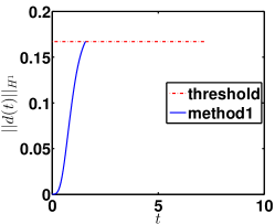
(a) Method 1

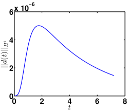
(b) Method 2

(c) Method 3

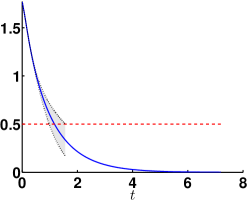
(d) Smallness Method 1

(e) Smallness Method 2

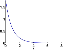
(f) Smallness Method 3

(g) $\|\varphi_{xx}\|_{L^{\infty}}$

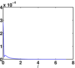
(h) $\|\operatorname{Res}\|_{H^{-1}}$

(i) $\varphi$

Figure 1: Initial value $u(x,0)=\sin(x)$, $N=128$ Fourier modes and step-size $h=10^{-5}$. Methods 2 and 3 show global existence as they stay bounded until time $T^{*}$ and even fulfill the smallness criterion before time $T^{*}$. Method 1 fails as it hits its threshold at approximately $t=1.5<T^{*}$ and also before the smallness criterion is reached.

In Figure 1 we have an initial value of $u(x,0)=\sin(x)$, $N=128$ Fourier modes and a step-size of $h=10^{-5}$. As Methods 2 and 3 stay bounded up to time $T^{*}$, we have global existence. Method 1 fails because it hits its threshold at approximately $t=1.5$, which is smaller than $T^{*}$. In the “Smallness plots” (Figures 1d, 1e and 1f) the grey area is the area around $\|\varphi(t)\|_{H^{1}}$ (the solid line) with distance $\|d(t)\|_{H^{1}}$, which is calculated by the respective method. The dashed line is the critical value $\varepsilon_{0}=\frac{1}{2}$. As the order of $\|d(t)\|_{H^{1}}$ is $10^{-6}$ for Methods 2 and 3, this area is not really visible in Figures 1e and 1f. An interesting detail is, that in Figure 1d it seems that the upper bound reaches $\varepsilon_{0}$, but in fact it is still a tiny bit above when Method 1 hits the threshold. To sum up, we have global regularity for this initial value from Methods 2 and 3 by smallness and time criteria, whereas both criteria fail for Method 1.

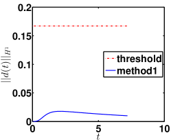
(a) Method 1

(b) Method 2

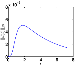
(c) Method 3

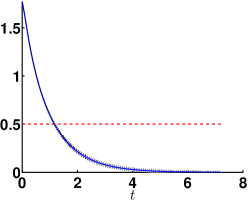
(d) Smallness Method 1

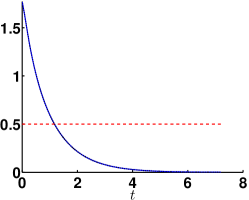
(e) Smallness Method 2

(f) Smallness Method 3

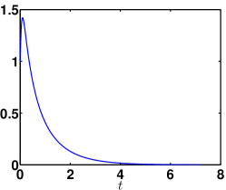
(g) $\|\varphi_{xx}\|_{L^{\infty}}$

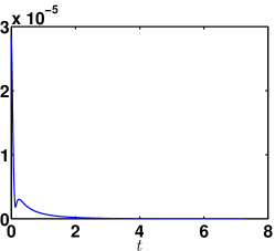
(h) $\|\operatorname{Res}\|_{H^{-1}}$

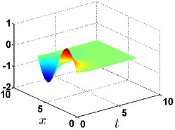
(i) $\varphi$

Figure 2: Same setting as in Figure 1, but now with smaller step-size $h=10^{-6}$. Now Method 1 shows global existence, too. Note that the order of the Residual decreased proportional to our step-size.

In Figure 2 we get global existence also with Method 1 by decreasing the stepsize to $h=10^{-6}$. All other parameters stay unchanged. Note that the order of the residual changed from $10^{-4}$ to $10^{-5}$ by the same factor we decreased the step-size.

Figure 3 also suggests that Method 1 is inferior to the other methods. With an already small step-size of $10^{-6}$ Method 1 does not get close to showing global existence, either by the smallness condition or the time condition.

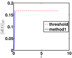
(a) Method 1

(b) Method 2

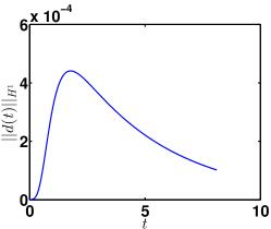
(c) Method 3

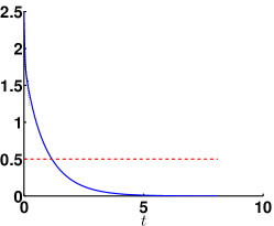
(d) Smallness Method 1

(e) Smallness Method 2

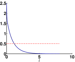
(f) Smallness Method 3

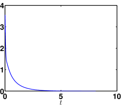
(g) $\|\varphi_{xx}\|_{L^{\infty}}$

(h) $\|\operatorname{Res}\|_{H^{-1}}$

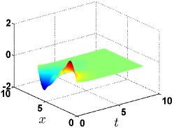
(i) $\varphi$

Figure 3: Initial value $u(x,0)=\sin(x)+\frac{1}{2}\sin(2x)$, $N=128$ Fourier modes and step-size $h=10^{-6}$. Method 1 reaches its threshold extremely fast. Methods 2 and 3 show global existence by both criteria.

In Table 1 we have collected some more results for different choices of initial data. One can see that if we have global existence by one criterion, then also by the other. The smallness criterion is also reached significantly earlier than the time criterion.

				Smallness			Time
$u(x,0)$	$T^{*}\approx$	N	h	M1	M2	M3	M1	M2	M3
$\sin(x)$	$7.1$	$128$	$10^{-5}$	–	$1.17$	$1.17$	$1.57$	✓	✓
$\sin(x)$	$7.1$	$128$	$10^{-6}$	$1.2$	$1.17$	$1.17$	✓	✓	✓
$\sin(x)+\frac{1}{2}\sin(2x)$	$8$	$128$	$10^{-6}$	–	$1.17$	$1.17$	$0.22$	✓	✓
$\cos(x)-\frac{1}{2}\sin(2x)+\frac{1}{3}\cos(3x)$	$8.3$	$128$	$10^{-6}$	–	$1.2$	$1.2$	$0.1$	✓	✓
$\sin(2x)$	$7.1$	$128$	$10^{-6}$	–	$0.12$	$0.12$	$0.4$	✓	✓
$2\sin(x)$	$14.2$	$128$	$10^{-6}$	–	–	–	$0.76$	$0.14$	$0.14$
$\frac{3}{2}\cos(x)-\frac{1}{2}\sin(2x)+\frac{1}{3}\cos(3x)$	$11.5$	$128$	$10^{-6}$	–	–	–	$0.03$	$0.15$	$0.15$

Table 1: All values are rounded to fit into the table. A ”–” in the ”Smallness” columns means, that the smallness criterion was not met by the respective method. Else there is the time when it was met. For the ”Time” columns this turns around. If the time criterion was met, the respective method gets a ”$\checkmark$”, else the time of the blowup / reaching the threshold.

As the bounds from Methods 2 and 3 are in all of our simulations almost identical, we need an artificial example to illustrate the difference between those methods. In Figure 4 we do this by artificially setting a constant, relatively large $\|\operatorname{Res}(t)\|_{H^{-1}}$ and an also constant, but smaller second derivative $\|\varphi_{xx}\|_{L^{\infty}}$, without using any numerical approximation. In this case Method 3 delivers the largest time interval as it stays finite up to $T\approx 0.16$, whereas Method 2 has a blowup at $T\approx 0.11$ and Method 1 at $T\approx 0.03$.

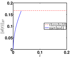
(a) Method 1

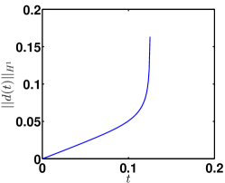
(b) Method 2

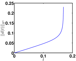
(c) Method 3

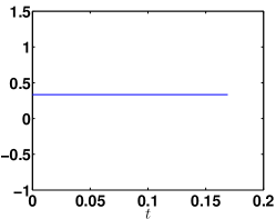
(d) $\|\varphi_{xx}\|_{L^{\infty}}$

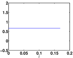
(e) $\|\operatorname{Res}\|_{H^{-1}}$

Figure 4: Artificial example for large fixed residual and not too large fixed second derivative. Method 3 is superior, but all methods do blow up relatively fast, as the residual is large.

6 Conclusion

We presented a method to verify global existence and uniqueness by combining a-posteriori numerical data and a-priori estimates. Therefore we prove a differential inequality for the error from the data to the true solution, having coefficients depending only on the numerical data. Three methods are presented to evaluate rigorously the analytic upper bounds for the error from these differential inequalities.

The third method seems to be the best, as it provides rigorous upper bounds and converges to a solution of the equality in the differential inequality. Nevertheless, in all practical examples with our Galerkin approximation, Methods 2 and 3 have shown nearly indistinguishable results.

While our proofs are rigorous, the implementation of the verification methods are not completely rigorous since we neglected rounding errors. Our analysis and computations suggest that numerical verification of regularity is feasible and can obtain global existence for initial conditions that are not covered by current analytical results.

We plan to perform a fully rigorous numerical verification in a future paper, using interval arithmetic to keep track of truncation errors. Moreover, replacing the a-priori estimates of the linearized operator by rigorous numerical estimates for its spectrum looks promising.

References

• [1] Dirk Blömker, Franco Flandoli, and Marco Romito. Markovianity and ergodicity for a surface growth PDE. Ann. Probab., 37(1):275–313, 2009.
• [2] Dirk Blömker and Marco Romito. Regularity and blow up in a surface growth model. Dyn. Partial Differ. Equ., 6(3):227–252, 2009.
• [3] Dirk Blömker and Marco Romito. Local existence and uniqueness in the largest critical space for a surface growth model. NoDEA, Nonlinear Differ. Equ. Appl., 19(3):365–381, 2012.
• [4] Sergei I. Chernyshenko, Peter Constantin, James C. Robinson, and Edriss S. Titi. A posteriori regularity of the three-dimensional Navier-Stokes equations from numerical computations. J. Math. Phys., 48(6):065204, 15 p., 2007.
• [5] Peter Constantin and Ciprian Foias. Navier-Stokes Equations. University of Chicago Press, 1988.
• [6] R. Cuerno, L. Vázquez, and R. Gago. Self-organized ordering of nanostructures produced by ion-beam sputtering. Phys. Rev. Lett., 94:016102, 4 p., 2005.
• [7] Masoumeh Dashti and James C. Robinson. An a posteriori condition on the numerical approximations of the Navier-Stokes equations for the existence of a strong solution. SIAM J. Numer. Anal., 46(6):3136–3150, 2008.
• [8] Sarah Day, Jean-Philippe Lessard, and Konstantin Mischaikow. Validated continuation for equilibria of PDEs. SIAM J. Numer. Anal., 45(4):1398–1424, 2007.
• [9] H. Koch and D. Tataru. Well-posedness for the Navier-Stokes equations. Adv. Math., 157(1):22–35, 2001.
• [10] Jean Leray. Sur le mouvement d’un liquide visqueux emplissant l’espace. Acta Math., 63:193–248, 1934.
• [11] Stanislaus Maier-Paape, Ulrich Miller, Konstantin Mischaikow, and Thomas Wanner. Rigorous numerics for the Cahn-Hilliard equation on the unit square. Rev. Mat. Complut., 21(2):351–426, 2008.
• [12] Carlo Morosi and Livio Pizzocchero. On approximate solutions of semilinear evolution equations. II: Generalizations, and applications to Navier-Stokes equations. Rev. Math. Phys., 20(6):625–706, 2008.
• [13] Carlo Morosi and Livio Pizzocchero. An $H^{1}$ setting for the Navier-Stokes equations: quantitative estimates. Nonlinear Anal., Theory Methods Appl., Ser. A, Theory Methods, 74(6):2398–2414, 2011.
• [14] Carlo Morosi and Livio Pizzocchero. On approximate solutions of the incompressible Euler and Navier-Stokes equations. Nonlinear Anal., Theory Methods Appl., Ser. A, Theory Methods, 75(4):2209–2235, 2012.
• [15] Mitsuhiro T. Nakao and Kouji Hashimoto. A numerical verification method for solutions of nonlinear parabolic problems. J. Math-for-Ind., 2009.
• [16] Mitsuhiro T. Nakao, Takehiko Kinoshita, and Takuma Kimura. On a posteriori estimates of inverse operators for linear parabolic initial-boundary value problems. Computing, 94(2-4):151–162, 2012.
• [17] Michael Plum. Existence and multiplicity proofs for semilinear elliptic boundary value problems by computer assistance. Jahresber. Dtsch. Math.-Ver., 110(1):19–54, 2008.
• [18] M. Raible, S. J. Linz, and P. Hänggi. Amorphous thin film growth: Minimal deposition equation. Phys. Rev. E, 62:1691–1694, 2000.
• [19] James C. Robinson, Pedro Marín-Rubio, and Witold Sadowski. Solutions of the 3D Navier–Stokes equations for initial data in $\dot{H}^{\frac{1}{2}}$ : robustness of regularity and numerical verification of regularity for bounded sets of initial data in $\dot{H}^{1}$ . J. Math. Anal. Appl., 400(1):76–85, 2013.
• [20] James C. Robinson and Witold Sadowski. Numerical verification of regularity in the three-dimensional Navier-Stokes equations for bounded sets of initial data. Asymptotic Anal., 59(1-2):39–50, 2008.
• [21] M. Siegert and M. Plischke. Solid-on-solid models of molecular-beam epitaxy. Physical Review E, 50:917–931, 1994.
• [22] Michael Winkler. Global solutions in higher dimensions to a fourth order parabolic equation modeling epitaxial thin film growth. Zeitschrift für angewandte Mathematik und Physik, 62(4):575–608, 2011.
• [23] Piotr Zgliczyński. Rigorous numerics for dissipative PDEs. III: An effective algorithm for rigorous integration of dissipative PDEs. Topol. Methods Nonlinear Anal., 36(2):197–262, 2010.