Adaptive Epidemic Dynamics in Networks: Thresholds and Control

Abstract

Theoretical modeling of computer virus/worm epidemic dynamics is an important problem that has attracted many studies. However, most existing models are adapted from biological epidemic ones. Although biological epidemic models can certainly be adapted to capture some computer virus spreading scenarios (especially when the so-called homogeneity assumption holds), the problem of computer virus spreading is not well understood because it has many important perspectives that are not necessarily accommodated in the biological epidemic models. In this paper we initiate the study of such a perspective, namely that of adaptive defense against epidemic spreading in arbitrary networks. More specifically, we investigate a non-homogeneous Susceptible-Infectious-Susceptible (SIS) model where the model parameters may vary with respect to time. In particular, we focus on two scenarios we call semi-adaptive defense and fully-adaptive defense, which accommodate implicit and explicit dependency relationships between the model parameters, respectively. In the semi-adaptive defense scenario, the model’s input parameters are given; the defense is semi-adaptive because the adjustment is implicitly dependent upon the outcome of virus spreading. For this scenario, we present a set of sufficient conditions (some are more general or succinct than others) under which the virus spreading will die out; such sufficient conditions are also known as epidemic thresholds in the literature. In the fully-adaptive defense scenario, some input parameters are not known (i.e., the aforementioned sufficient conditions are not applicable) but the defender can observe the outcome of virus spreading. For this scenario, we present adaptive control strategies under which the virus spreading will die out or will be contained to a desired level.

Author’s address: Shouhuai Xu, Li Xu, and Zhenxin Zhan are with the Department of Computer Science, University of Texas at San Antonio. Corresponding author: Shouhuai Xu (shxu@cs.utsa.edu).
Wenlian Lu is with the Center for Computational Systems Biology and the School of Mathematical Sciences, Fudan University (wenlian@fudan.edu.cn).

1 Introduction

Theoretically modeling the spreading dynamics of computer virus (or malware such as worm and bot) is important for deepening our understanding and for designing effective, if not optimal, defenses. We observe, however, that the utility of theoretical modeling in this context is not well understood yet because existing models are often adapted from biological epidemic ones. As a consequence, many existing models of computer virus spreading dynamics made the so-called homogeneity assumption, which roughly says that the nodes are equally powerful in infecting others. Realizing the limitation of the assumption, there have been investigations that aim to weaken the assumption by considering heterogeneous network topology (where different nodes may have different infection capabilities because they have different degrees). Along this line of study, the present paper moves a step further by exploring models that accommodate realistic scenarios where the model parameters may change over time (i.e., the parameters are some functions of time), which captures the fact that both attack and defense are dynamically evolving or under dynamical adjustment and reflects the persistence of virus spreading. This allows us to investigate an important and novel perspective of virus spreading-defense dynamics, namely that of adaptive defense against computer virus spreading.

1.1 Our Contributions

We investigate a non-homogeneous Susceptible-Infectious-Susceptible (SIS) model in arbitrary networks (i.e., there is no restriction on the topology of the spreading networks and the nodes may have different defense or cure capabilities). The model can accommodate both semi-adaptive defense and fully-adaptive defense. In the semi-adaptive defense scenario, the input parameters in the model are known and can vary with respect to time (e.g., according to some deterministic functions of time or according to some stochastic process, but we do not impose any practical restrictions on the types of functions). For this scenario, we present a set of sufficient conditions, from general to specific (but more succinct), under which the virus spreading will die out. We note that such sufficient conditions are also known as epidemic thresholds in the literature.

In the fully-adaptive defense scenario, some input parameters are not known and thus the aforementioned sufficient conditions are not applicable. Nevertheless, the defender might be able to observe the outcome of virus spreading (i.e., which nodes are infected at a point in time). For this scenario, we present adaptive control strategies under which the virus spreading will die out or will be contained to a desired level (which is important when, for example, the price to kill the virus spreading may be too high).

Because of the above, our model supersedes previous homogeneous and non-homogeneous models that offered relevant analytical insights; the concrete connection will be made when the need arises. Our analytical results are confirmed via simulation, from which we draw additional observations that serve as hints for future modeling studies. We discuss the practical implications of our model and the derived insights as well.

Finally, we note that the present paper is meant to explore theoretical characterizations of spreading-defense dynamics while assuming certain parameters can be observed or measured (e.g., based on extensive data and possibly expert knowledge). This may not be feasible some times. Regardless, we believe that such studies are important on their own and represent a necessary step towards the ultimate characterization of virus spreading-defense dynamics (which in turn helps design more effective or even optimal defenses).

1.2 Related Work

To the best of our knowledge, there are no existing studies on modeling adaptive spreading-defense dynamics in arbitrary networks. The work that is most closely related to ours was due to Chakrabarti et al. [Chakrabarti et al. (2008)], who considered computer virus spreading in arbitrary networks — a scenario also investigated in [Wang et al. (2003), Ganesh et al. (2005)]. The most important contribution of these studies is the identification of a sufficient condition (i.e., epidemic threshold) under which the virus spreading will die out; we will discuss the relationship between their result and ours when the need arises. Earlier studies either made the homogeneity assumption (e.g., [Kephart and White (1991), Kephart and White (1993)]) as in biological epidemic models (see, for example, [McKendrick (1926), Kermack and McKendrick (1927), Bailey (1975), Anderson and May (1991), Hethcote (2000)]), or considered specific non-homogeneous networks [Chakrabarti et al. (2008)].

We should mention prior work that is conceptually or spiritually relevant. The concept of “adaptable robust computer systems” was investigated by Bhargava et al. [Bhargava et al. (1986)], which however has a very different meaning and is for very different purposes. Also for a different purpose, Zou et al. [Zou et al. (2005)] explored the concept of “adaptive defense” based on cost optimization, where cost was introduced by false positives and false negatives. In particular, they considered optimal adaptive defense against worm infection, but is from the perspective of decision whether or not to block/allow some specific host traffic. As such, it may be possible to combine their studies and ours because we do not consider cost.

Outline: In Section 2 we present our model as well as the analytical insights. We report our simulation study in Section 3. We conclude the paper in Section 4 with open problems.

2 Adaptive Epidemic Dynamics: Model and Analysis

2.1 The model

Primary parameters. Because we want to accommodate spreading in arbitrary networks, we assume that virus spreads over a series of finite, dynamical graphs $G(t)=(V,E(t))$, where $V$, $|V|=n$, is the set of nodes or vertices and $E(t)$ is the set of (possibly changing) edges or arcs at time $t\geq 0$ (i.e., the topology may change with respect to time). At any time $t$, an infected node $u$ can directly infect node $v$ if $(u,v)\in E(t)$. Denote by $A(t)=[a_{vu}(t)]$ the adjacency matrix of $G(t)$, where $a_{vv}(t)=0$ for all $v\in V$, and $a_{vu}(t)=1$ if and only if $(u,v)\in E(t)$. Note that this representation naturally accommodates both directed and undirected topologies, and thus our results equally apply to them.

A node $v\in V$ is susceptible if $v$ is secure but vulnerable, and infected if $v$ is successfully attacked (i.e., infected and infectious). At any time $t$, a node $v\in V$ is either susceptible or infected. Moreover, a susceptible node may become infected because of some infected node $u$ where $(u,v)\in E(t)$, and an infected node may become susceptible because of cure. Since an infected node may become susceptible again, our model falls into the category of the so-called SIS models, but our model has the unique feature that values of the parameters can change with respect to time.

We consider two dependent variables: $s_{v}{(t)}$, the probability $v\in V$ is susceptible at time $t$; $i_{v}{(t)}$, the probability $v\in V$ is infected at time $t$. We consider a continuous-time model, which preserves the invariant $s_{v}{(t)}+i_{v}{(t)}=1$. The model’s input parameters are:

• $\beta_{v}(t)$: The probability an infected node $v$ becomes susceptible at time $t$.

• $\gamma_{uv}(t)$: The probability an infected node $u$ successfully infects a susceptible node $v$ over edge $(u,v)\in E(t)$ at time $t$. For simplicity, we assume that $\gamma_{uv}(t)=\gamma(t)$ for all $(u,v)\in E(t)$.

For the sake of mathematical rigorousness, the $\beta_{v}(t)$’s and the $\gamma_{uv}(t)$’s, which are probabilities, should be “measurable” so as to ensure the existence of solutions to system (2.4) and be “bounded” so as to ensure the proof of Theorem 2.3 can get through. To avoid any unnecessary mathematical subtleties, we simply assume that these parameters are “boundedly measurable,” which has no consequence in practice. Note that $A(t)$ is naturally bounded.

Other parameters and notations. Below is a summary of the major notations used in the paper; notations only occasionally used are explained when the need arises.

model input parameters:
$A(t)=[a_{vu}(t)]$	the adjacency matrix of graph $G(t)=(V,E(t))$ where $|V|=n$, and $a_{vu}(t)=1$ if and only if $(u,v)\in E(t)$. Moreover, $a_{vv}(t)=0$ for all $v\in V$.
$\beta_{v}(t)$	the cure capability of node $v$ at time $t$
$\gamma(t)$	the edge infection capability at time $t$
dependent variables:
$s_{v}{(t)}$	the probability node $v\in V$ is susceptible at time $t$
$i_{v}{(t)}$	the probability node $v\in V$ is infected at time $t$
intermediate variables:
$\delta_{v}{(t)}$	the probability susceptible $v\in V$ becomes infected at time $t$ because of infected neighbors $\{u:(u,v)\in E(t)\}$
other notations:
$\lambda_{1}$	the largest (in modulus) eigenvalue of adjacency matrix $A$
$\|\cdot\|$	the 1-norm of vector or matrix
$B(t)=\text{\text{diag}}[\beta_{1}(t),\cdots,\beta_{n}(t)]$	the cure probability diagonal matrix

The state transition diagram and master equation. Figure 1 depicts the state transition diagram of a node, where the probability $\delta_{v}{(t)}$ is given by

$$\delta_{v}{(t)}=1-\prod\limits_{(u,v)\in E(t)}\left[1-\gamma(t)\cdot i_{u}{(t)}\right].$$ (2.1)

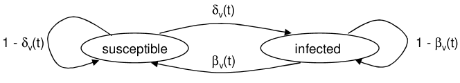
Figure 1: State transition diagram of node $v\in V$ at time $t$

Note that in the derivation of Eq. (2.1), we assumed that the events that infected neighbors infect a node are independent. Note also that $s_{v}(t)+i_{v}(t)=1$ for any $t$. Based on the state transition diagram we obtain the following master equation of dynamics:

$$\frac{di_{v}(t)}{dt}=\bigg{[}1-\prod_{u\in V}[1-\gamma(t)a_{vu}(t)i_{u}{(t)}]\bigg{]}[1-i_{v}{(t)}]-\beta_{v}(t)i_{v}{(t)},$$ (2.2)

where $a_{vu}(t)=1$ if and only if $(u,v)\in E(t)$.

2.2 Sufficient conditions for dying out in the scenario of semi-adaptive defense

In this subsection we present a set of sufficient conditions under which the virus spreading will die out. The sufficient conditions are applicable when the model’s input parameters, namely the $\beta_{v}(t)$’s and $\gamma(t)$ are given. Moreover, it is possible that $\beta_{v}(t)$ relies on $\gamma(t)$; for example, the former is an (implicit) function of the latter. This explains why we call this scenario the semi-adaptive defense.

Theorem 1

(a general sufficient condition under which virus spreading dies out) Consider the following comparison (and linearization) system of Eq. (2.2):

$$\frac{dx_{v}(t)}{dt}=\sum_{u=1}^{n}a_{vu}(t)\gamma(t)x_{u}(t)-\beta_{v}(t)x_{v}{(t)}.$$ (2.3)

Let $x(t)=[x_{1}(t),\cdots,x_{n}(t)]^{\top}$, we obtain the following compact form of Eq. (2.3):

$$\frac{dx(t)}{dt}=\bigg{[}\gamma(t)A(t)-B(t)\bigg{]}x(t).$$ (2.4)

Denote by $U(t,t^{\prime})$ the solution matrix of linear system (2.4), namely that each solution of linear system (2.4), $x(t)$, with initial condition $x(t_{0})=x_{0}$, can be written as $x(t)=U(t,t_{0})x_{0}$. Because the solution $x(t)$ is dependent upon the initial value $x_{0}$ but the solution matrix $U(t,t^{\prime})$ is not, the corresponding maximum Lyapunov exponent (MLE) is determined by the solution matrix (rather than by the solution $x(t)$) and can be defined as [Oseledec (1968)]:

$$\mu=\lim_{t\to\infty}\frac{1}{t}\ln\|U(t,0)\|$$

where $\|\cdot\|$ is (for specificality) the 1-norm of matrix (because $\mu$ is independent of the choice of the norm). If $\mu<0$, the virus spreading will die out regardless of the initial infection configuration; if $\mu>0$ and system (2.4) is ergodic [Oseledec (1968)], the virus spreading will not die out in some initial infection configurations (i.e., “the equilibrium of $i^{*}=0$ is unstable” in mathematical terms).

Proof 2.2.

Note that

$$1-\prod_{u\in V}[1-\gamma(t)a_{vu}(t)i_{u}(t)]\leq\gamma(t)\sum_{u\in V}a_{vu}(t)i_{u}(t).$$ (2.5)

If $i_{v}(0)=x_{v}(0)$ for all $v\in V$, then the comparison system (2.3) satisfies that $i_{v}(t)\leq x_{v}(t)$ holds for all $t\geq 0$ and $v\in V$. Since Eq. (2.3) is actually the linear system of the system (2.2) at $i_{v}=0$ for all $v\in V$. Therefore, we can conclude that the stability of Eq. (2.2) is equivalent to that of Eq. (2.3). In other words, if all $x_{v}(t)$’s of system (2.3) converge to zero, then system (2.2) is stable regardless of the initial values; on the other hand, if system (2.3) is unstable, then system (2.2) is also unstable. If system (2.4) is ergodic [Oseledec (1968)], then the limit $\mu$ exists; otherwise, we can alternatively define $\mu=\overline{\lim}_{t\to\infty}\frac{1}{t}\ln\|U(t,0)\|$, where $\overline{\lim}_{t\to\infty}z(t)$ represents the upper bound of the limit of $z(t)$ as $t$ goes to infinity, is also guaranteed to exist. In any case, by applying the definition of MLE, we obtain the theorem immediately.

Discussion. The above sufficient condition $\mu<0$ for the virus spreading to die out is actually close to being necessary, meaning that if $\mu>0$, then the virus spreading will not die out in most, rather than just some, initial infection configurations. According to the Lyapunov exponent and smooth ergodic theory developed by [Pesin (1977)] and many others, $\mu>0$ means that the system (2.2) possesses an unstable manifold, which implies that the stable manifold, i.e., the set of points (i.e., the initial values) starting from which the system (2.2) converges to the origin, has dimension less than $n$. Therefore, the stable manifold has Lesbegue measure $0$. That is, except a set with Lesbegue measure $0$, the virus spreading never dies out with respect to any initial infection configuration.

The sufficient condition given in Theorem 1 is very general because in its derivation no “amplification” is used and dynamical topology $E(t)$ is accommodated. However, it requires to, among other things, solve a system of $n$ linear equations of $n$ variables (equivalently, diagonalizing a $n\times n$ matrix), which can be quite time-consuming for large $n$ (the number of nodes). In what follows we give two succinct sufficient conditions, which can be easily connected to previous state-of-the-art results.

Theorem 2.3.

(a succinct sufficient condition) Suppose $\beta_{v}(t)=\beta(t)$ for all $v\in V$ (i.e., all nodes have the same cure capability) and $E(t)=E$ for any time $t$, meaning that the topology does not change over time and $A=A(t)$ for any $t$. Consider the system

$$\frac{dx(t)}{dt}=\bigg{[}\gamma(t)A-\beta_{v}(t)I_{n}\bigg{]}x(t),$$ (2.6)

where $I_{n}$ is the $n\times n$ identity matrix. Let

$$\bar{\gamma}=\lim_{t\to\infty}\frac{1}{t}\int_{t_{0}}^{t+t_{0}}\gamma(\tau)d\tau,~{}~{}~{}\bar{\beta}=\lim_{t\to\infty}\frac{1}{t}\int_{t_{0}}^{t+t_{0}}\beta(\tau)d\tau,$$

and suppose the limits exist and are uniform with respect to $t_{0}$. Let $\lambda_{1}$ be the largest (in modulus) eigenvalue of $A$. If

$$\lambda_{1}<\frac{\bar{\beta}}{\bar{\gamma}},$$ (2.7)

then the virus spreading will die out regardless of the initial infection configuration; if

$$\lambda_{1}>\frac{\bar{\beta}}{\bar{\gamma}},$$ (2.8)

then the virus spreading will not die out in some initial infection configurations.

Proof 2.4.

Consider system (2.4). Let $A=S^{-1}JS$ be the Jordan canonical form with

$$J=\left[\begin{array}[]{lllll}J_{1}&&&&\\ &J_{2}&&&\\ &&J_{3}&\\ &&&\ddots&\\ &&&&J_{K}\end{array}\right],~{}J_{k}=\left[\begin{array}[]{lllll}\lambda_{k}&0&0&\cdots&0\\ 1&\lambda_{k}&0&\cdots&0\\ 0&1&\lambda_{k}&\cdots&0\\ \vdots&\vdots&\vdots&\ddots&\vdots\\ 0&0&\cdots&1&\lambda_{k}\end{array}\right],$$

where $\lambda_{k}$, $k=1,\cdots,K$, are the distinct eigenvalues of $A$. Recall that $\lambda_{1}$ is the largest eigenvalue in modulus. From the Perron-Frobenius theorem [Berman and Shaked-Monderer (2003)], $\lambda_{1}$ is a real number. Then, letting $y(t)=Sx(t)$, we have

$$\frac{dy(t)}{dt}=[\gamma(t)J-\beta(t)I_{n}]y(t).$$

Namely,

$$\frac{dy_{v}(t)}{dt}=[\gamma(t)\lambda_{k_{v}}-\beta(t)]y_{v}(t)+\xi_{v}(t),$$

where $\lambda_{k_{v}}$ is the eigenvalue of $A$ corresponding to the Jordan block $J_{k_{v}}$ that contains column $v$, and $\xi_{v}(t)=0$ if the $v$-th row of $S$ is an eigenvector of $A$ and $\xi_{v}(t)=\gamma(t)y_{v-1}(t)$ otherwise. First, consider $v=1$ corresponding to the eigenvalues $\lambda_{1}$. We have

$$y_{1}(t)=y_{1}(0)\exp\left(\int_{0}^{t}[\gamma(\tau)\lambda_{1}-\beta(\tau)]d\tau\right).$$ (2.10)

One can see that the Lyapunov exponent of system (2.10) is calculated as

$$\lim_{t\to\infty}\frac{1}{t}\ln||y_{1}(t)|| = \lim_{t\to\infty}\frac{1}{t}\ln||y_{1}(0)||+\lim_{t\to\infty}\frac{1}{t}\int_{0}^{t}[\gamma(\tau)\lambda_{1}-\beta(\tau)]d\tau$$

$$= 0+\bar{\gamma}\lambda_{1}-\bar{\beta}<0,$$

which implies $\lim_{t\to\infty}y_{1}(t)=0$.

Assuming $\lim_{t\to\infty}y_{v}(t)=0$ already proved, consider $y_{v+1}(t)$. We have

$$y_{v+1}(t)=y_{v+1}(0)\exp\left(\int_{0}^{t}k(\tau)d\tau\right)+\int_{0}^{t}\xi_{v+1}(a)\exp\left(\int_{a}^{t}k(\tau)d\tau\right)da$$

where $k(\tau)=\gamma(\tau)\lambda_{k_{v+1}}-\beta(\tau)$. From condition (2.7), there exists a sufficiently small $\epsilon>0$ such that $(\bar{\gamma}+\epsilon)\lambda_{1}-(\bar{\beta}+\epsilon)<0$. Let $\varphi=-(\bar{\gamma}+\epsilon)\lambda_{1}+(\bar{\beta}+\epsilon)$. One can see that $\varphi>0$. Since the limits $\int_{t_{0}}^{t_{0}+t}\beta(\tau)d\tau$ and $\int_{t_{0}}^{t_{0}+t}\gamma(\tau)d\tau$ are uniform with respect to $t_{0}$, there exists $T>0$ such that

$$\frac{1}{t-a}\int_{a}^{t}\beta(\tau)d\tau<\bar{\beta}+\epsilon,~{}\frac{1}{t-a}\int_{a}^{t}\gamma(\tau)d\tau<\bar{\gamma}+\epsilon$$

hold for any $a$ and $t$ with $t-a>T$. Let ${\mathcal{R}e}(z)$ denote the real part of a complex number $z$. Then, we have

$$\mathcal{R}e\bigg{(}\frac{1}{t-a}\int_{a}^{t}k(\tau)d\tau\bigg{)} = \frac{1}{t-a}\int_{a}^{t}[\gamma(\tau)\mathcal{R}e(\lambda_{k_{v+1}})-\beta(\tau)]d\tau$$

$$\leq \frac{1}{t-a}\int_{a}^{t}[\gamma(\tau)\lambda_{1}-\beta(\tau)]d\tau$$

$$\leq (\bar{\gamma}+\epsilon)\lambda_{1}-(\bar{\beta}+\epsilon)=-\varphi<0$$

for all $t$ and $a$ with $t-a>T$. This implies that the first term $y_{v+1}(0)\exp(\int_{0}^{t}k(\tau)d\tau)$ converges to zero. Let $M>0$ be a constant such that $\sup\limits_{\tau,j}|\gamma(\tau)\lambda_{j}-\beta(\tau)|<M$. For the second term, we have

$$\bigg{|}\int_{0}^{t}\xi_{v+1}(a)\exp\left(\int_{a}^{t}k(\tau)d\tau\right)da\bigg{|}$$

$$= \bigg{|}\int_{0}^{t-T}\xi_{v+1}(a)\exp\left(\int_{a}^{t}k(\tau)d\tau\right)da+\int_{t-T}^{t}\xi_{v+1}(a)\exp\left(\int_{a}^{t}k(\tau)d\tau\right)da\bigg{|}$$

$$\leq \int_{0}^{t-T}|\xi_{v+1}(a)|\exp\left(-\varphi(t-a)\right)da+\int_{t-T}^{t}|\xi_{v+1}(a)|\exp(MT)da.$$

In the case of $\xi_{v+1}(t)=0$, we immediately conclude that $\lim_{t\to\infty}y_{v+1}(t)=0$. Otherwise, according to the condition and the L’Hospital principle, we have

$$\lim_{t\to\infty}\int_{0}^{t-T}|\xi_{v+1}(a)|\exp\big{[}-\varphi(t-a)\big{]}da = \lim_{t\to\infty}\frac{\int_{0}^{t-T}|\xi_{v+1}(a)|\exp(\varphi a)da}{\exp(\varphi t)}$$

$$= \lim_{t\to\infty}\frac{|\xi_{v+1}(t-T)|\exp(\varphi(t-T))}{\varphi\exp(\varphi t)}$$

$$= \lim_{t\to\infty}\frac{|y_{v}(t-T)\gamma(t-T)|\exp(-\varphi T))}{\varphi}=0,$$

due to the assumption $\lim_{t\to\infty}y_{v}(t)=0$. We also have

$$\lim_{t\to\infty}\int_{t-T}^{t}|\xi_{v+1}(a)|\exp(MT)da=0.$$

Therefore, we can conclude $\lim_{t\to\infty}y_{v+1}(t)=0$.

Note that condition (2.8) implies that system (2.4) is unstable. Since system (2.4) is in fact the linearization system of Eq. (2.2), we can conclude that system (2.2) is unstable under condition (2.8). This completes the proof. ∎

If $\beta(t)$ and $\gamma(t)$ are ergodic stochastic processes, from the multiplicative ergodic theory of the random dynamical systems [Arnold (1998)], we have the following result as a corollary of Theorem 2.3.

Corollary 2.5.

(another succinct sufficient condition) Suppose $\beta_{v}(t)=\beta(t)$ for all $v\in V$ (i.e., all nodes have the same cure capability) and $E(t)=E$ for any time $t$ (i.e., topology does not change over time). Suppose $\{\beta(t)\}_{t\geq 0}$ and $\{\gamma(t)\}_{t\geq 0}$ are ergodic stochastic processes (i.e., $\beta(t)$ and $\gamma(t)$ are some random variables). Let ${\sf E}(\beta(0))$ and ${\sf E}(\gamma(0))$ be the expectations with respect to the stationary distributions of the respective ergodic stochastic process. Suppose the convergences

$${\sf E}(\beta(0))=\frac{1}{t}\int_{t_{0}}^{t_{0}+t}\beta(\tau)d\tau,~{}{\sf E}(\gamma(0))=\frac{1}{t}\int_{t_{0}}^{t_{0}+t}\gamma(\tau)d\tau,$$

are both uniform with respect to $t_{0}$ almost surely. If

$$\lambda_{1}<\frac{{\sf E}(\beta(0))}{{\sf E}(\gamma(0))},$$

the spreading will die out almost surely regardless of the initial infection configuration; if

$$\lambda_{1}>\frac{{\sf E}(\beta(0))}{{\sf E}(\gamma(0))},$$

the spreading will not die out in some initial infection configurations.

Discussion. The state-of-the-art sufficient condition for the dying out of virus spreading in an arbitrary network is $\lambda_{1}<\frac{\beta}{\gamma}$, which was given in [Chakrabarti et al. (2008)]. In the setting of [Chakrabarti et al. (2008)], the parameters satisfy that $\beta_{v}(t)=\beta$ for all $v\in V$ and all $t$, and $\gamma(t)=\gamma$ for all $t$. As such, their result is clearly a special case of the above Corollary 2.5 (note that it is guaranteed that ${\sf E}(\gamma(0))\neq 0$), and thus of the above Theorem 2.3.

2.3 Adaptive control in the scenario of fully-adaptive scenario

In the semi-adaptive defense scenario investigated above, we assumed that the parameters $\gamma(t)$ and $\beta_{v}(t)$ are given. What if they are not given? In what follows we investigate a representative scenario, where the defender is not given $\gamma(t)$ but can observe $i_{v}(t)$. Specifically, we consider two sufficient conditions of adaptive control: one under which the virus spreading will die out (Section 2.3.1), and another under which the virus spreading will not die out but will be contained to a desired level of infection (Section 2.3.2).

2.3.1 Sufficient condition under which the virus spreading dies out under adaptive control

The question we ask is: How should the defender adjust the defense, namely how $\beta_{v}(t)$ should depend upon $i_{v}(t)$, so that the virus spreading will die out? We assume for concreteness that $\beta_{v}(0)=0$ for all $v\in V$; this accounts for the worst-case scenario.

Theorem 2.6.

(characterization of adaptive control strategy under which the virus spreading will die out) Suppose without loss of generality $\beta_{v}(0)=0$ for all $v\in V$. If

$$\frac{d\beta_{v}(t)}{dt}=\rho i_{v}(t),$$

where $\rho$ is an (almost) arbitrary positive constant, then the virus spreading will die out regardless of the initial infection configuration.

Proof 2.7.

Define a candidate Lyapunov function with respect to the infectious probabilities $i=[i_{1},\cdots,i_{n}]^{\top}$ and the cure capabilities $\tilde{\beta}=[\beta_{1},\cdots,\beta_{n}]^{\top}$:

$$V(i,\tilde{\beta})=\sum_{v=1}^{n}i_{v}(t)+\frac{1}{2\rho}\sum_{v=1}^{n}(\beta_{v}(t)-\beta_{0,v})^{2}.$$

Let $\beta_{0,v}$, $v=1,\cdots,n$, be positive constants satisfying

$$\beta_{0,v}>(n-1)\sup_{t}\gamma(t)+1,~{}\forall~{}v=1,\cdots,n$$

owing to the fact that $1\geq\gamma(t)\geq 0$. Due to inequality (2.5), differentiating $V(i,\tilde{\beta})$ gives

$$\frac{dV(i,\tilde{\beta})}{dt} = \sum_{v=1}^{n}\left[1-\prod_{(u,v)\in E{(t)}}(1-\gamma(t)i_{u}(t))\right](1-i_{v}(t))-\sum_{v=1}^{n}\beta_{v}(t)i_{v}(t)$$

$$+\sum_{v=1}^{n}(\beta_{v}(t)-\beta_{0,v})i_{v}(t)$$

$$\leq \sum_{v=1}^{n}\gamma(t)\sum_{u=1}^{n}a_{vu}(t)i_{u}(t)-\sum_{v=1}^{n}\beta_{v}(t)i_{v}(t)+\sum_{v=1}^{n}(\beta_{v}(t)-\beta_{0,v})i_{v}(t)$$

$$\leq \sum_{v=1}^{n}\gamma(t)\sum_{u=1}^{n}a_{vu}(t)i_{u}(t)-\sum_{v=1}^{n}\beta_{0,v}i_{v}(t)$$

$$\leq \gamma(t)(n-1)\sum_{u=1}^{n}i_{u}(t)-\sum_{v=1}^{n}\beta_{0,v}i_{v}(t)$$

$$\leq -\sum_{v=1}^{n}i_{v}(t).$$

According to the LaSalle principle [LaSalle (1960)], the system converges to the largest invariant set $\{(i,\tilde{\beta}):\sum_{v=1}^{n}i_{v}=0\}$, which implies $\lim_{t\to\infty}i_{v}(t)=0$ for all $v=1,\cdots,n$. ∎

The above Theorem 2.6 has the following implications.

Proposition 2.8.

We can bound from above the accumulated number of infected nodes in the long run (a node is counted multiple times if it is infected at multiple points in time) as follows:

$$\int_{0}^{\infty}\sum_{v=1}^{n}i(\tau)d\tau\leq\frac{(n-1)^{2}\gamma_{m}}{\rho}+\frac{n-1}{\rho}\sqrt{\sum_{v=1}^{n}i_{v}(0)+\frac{(n-1)^{3}\gamma_{m}^{2}}{2\rho}}$$ (2.11)

where $\gamma_{m}=\sup\limits_{t}\gamma(t)$ and $\beta_{0,m}=\min\limits_{v}\beta_{0,v}$.

Proof 2.9.

From the proof of Theorem 2.6, we have

$$\frac{dV(i,B)}{dt}\leq[\gamma_{m}(n-1)-\beta_{0,m}]\sum_{v=1}^{n}i_{v}(t),$$

which implies

$$\int_{0}^{t}\sum_{v=1}^{n}i_{v}(\tau)d\tau\leq\frac{1}{\beta_{0,m}-\gamma_{m}(n-1)}[V(0)-V(t)]\leq\frac{1}{\beta_{0,m}-\gamma_{m}(n-1)}V(0).$$

If $\beta_{v}(0)=0$ for all $v=1,\cdots,n$ and all $\beta_{v,0}$ are the same and are thus denoted by $\beta_{0}$, we have the following estimation:

$$\int_{0}^{\infty}\sum_{v=1}^{n}i(\tau)d\tau\leq\frac{1}{\beta_{0}-\gamma_{m}(n-1)}\big{[}\sum_{v=1}^{n}i_{v}(0)+\frac{1}{2\rho}(n-1)\beta_{0}^{2}\big{]}.$$

By setting

$$\beta_{0}=a+\frac{\sqrt{\sum_{v=1}^{n}i_{v}(0)+1/(2\rho)(n-1)^{3}\gamma_{m}^{2}}}{1/(2\rho)(n-1)},$$

we obtain the minimum of the right-hand side and thus complete the proof. ∎

Physical meanings of Proposition 2.8. The term at the left-hand side of inequality (2.11) captures, in addition to the aforementioned estimation of the total number of infected nodes in the network (counting repetition) over time, the convergence rate of the adaptive control strategy. This allows us to draw the following insights: (i) The larger $\rho$, the faster the virus spreading will die out; (ii) the larger degree of initial infection, the slower the virus spreading will die out; (iii) the larger edge infection probability $\gamma$, the slower the virus spreading will die out.

2.3.2 Adaptive control under which the virus spreading will not die out but will be contained to a desired level

In the above we have given some sufficient condition on adjusting the defense or $\beta_{v}(t)$ so that the virus spreading will die out. What if the required $\beta_{v}(t)$ cannot be achieved, meaning that we may not expect that the virus spreading die out? This is possible because the defense may not be as good as one may wish or because of budget limitation. In this case, we ask an alternative interesting question: What it takes so that $i_{v}(t)$ can converge or be contained to some pre-determined level of infection $i_{v}^{*}$?

Theorem 2.10.

(characterization of adaptive control strategy under which the virus spreading will be contained to a desired level of infection) Consider the following variant of the master equation Eq. (2.2),

$$\frac{di_{v}(t)}{dt} = \bigg{[}1-\prod_{(u,v)\in E}[1-\gamma\cdot i_{u}{(t)}]\bigg{]}(1-i_{v}{(t)})-\beta_{v}(t)i_{v}{(t)}+w_{v}$$ (2.12)

For any $1\geq i_{v}^{*}>0$, $v=1,\cdots,n$, letting

$$\beta_{v}^{*}=\frac{[1-\prod_{(u,v)\in E}(1-\gamma\cdot i_{u}^{*})](1-i_{v}^{*})}{i_{v}^{*}},$$

if we use the following adaptive control strategy

$$\frac{d\beta_{v}(t)}{dt}=\rho[i_{v}(t)-i_{v}^{*}]i_{v}(t),~{}~{}~{}~{}~{}~{}w_{v}=\eta[i_{v}^{*}-i_{v}(t)],$$

where $\rho$ is an (almost) arbitrary positive constant, and $\eta$ is a positive constant with $\eta+\min\limits_{v}\beta_{v}^{*}>1+(1-\gamma)\lambda_{1}$ where $\lambda_{1}$ is the largest (in modulus) eigenvalue of the adjacency matrix $A$, we have $\lim_{t\to\infty}i_{v}(t)=i_{v}^{*}$.

Proof 2.11.

From Perron-Frobenius theorem [Berman and Shaked-Monderer (2003)], we have that there exist some positive constants $P_{1},\cdots,P_{n}$ such that $P={\rm diag}[P_{1},\cdots,P_{n}]$ satisfies $[PA+A^{\top}P]\leq\lambda_{1}P$. Consider the candidate Lyapunov function with respect to $i=[i_{1},\cdots,i_{n}]^{\top}$ and $\tilde{\beta}=[\beta_{1},\cdots,\beta_{n}]^{\top}$:

$$V(i,\tilde{\beta})=\frac{1}{2}\sum_{v=1}^{n}P_{v}[i_{v}-i_{v}^{*}]^{2}+\frac{1}{2\rho}\sum_{v=1}^{n}P_{v}(\beta_{v}-\beta_{v}^{*})^{2}.$$

Differentiating $V(x,\tilde{\beta})$ gives

$$\frac{d{V}(i,\tilde{\beta})}{dt}$$

$$= \sum_{v=1}^{n}P_{v}[i_{v}(t)-i_{v}^{*}]\bigg{\{}[1-\prod_{(u,v)\in E}(1-\gamma\cdot i_{u}{(t)})](1-i_{v}{(t)})-\beta_{v}(t)i_{v}{(t)}-\eta(i_{v}-i_{v}^{*})\bigg{\}}$$

$$+\sum_{v=1}^{n}P_{v}(\beta_{v}(t)-\beta_{v}^{*})(i_{v}(t)-i_{v}^{*})i_{v}(t)$$

$$= \sum_{v=1}^{n}P_{v}[i_{v}(t)-i_{v}^{*}]\bigg{\{}\big{[}1-\prod_{(u,v)\in E}(1-\gamma\cdot i_{u}{(t)})\big{]}(1-i_{v}{(t)})$$

$$-\big{[}1-\prod_{(u,v)\in E}(1-\gamma\cdot i_{u}^{*})\big{]}(1-i_{v}^{*})-\beta_{v}(t)i_{v}{(t)}-\beta_{v}^{*}i_{v}^{*}+\eta(i_{v}-i_{v}^{*})\bigg{\}}$$

$$+\sum_{v=1}^{n}P_{v}(\beta_{v}(t)+\beta_{v}^{*})(i_{v}(t)-i_{v}^{*})i_{v}(t).$$

Note that

$$\bigg{|}[1-\prod_{(u,v)\in E}(1-\gamma\cdot i_{u}{(t)})](1-i_{v}{(t)})-[1-\prod_{(u,v)\in E}(1-\gamma\cdot i_{u}^{*})](1-i_{v}^{*})\bigg{|}$$

$$\leq \bigg{|}(i_{v}(t)-i_{v}^{*})\prod_{(u,v)\in E}(1-\gamma i_{v}(t))\bigg{|}+\bigg{|}(1-i_{v}^{*})\big{[}\prod_{(u,v)\in E}(1-\gamma i_{u}(t))-\prod_{(u,v)\in E}(1-\gamma i_{u}^{*})\big{]}\bigg{|}$$

$$\leq |i_{v}(t)-i_{v}^{*}|+\sum_{(u,v)\in E}|i_{u}(t)-i_{u}^{*}|\prod_{(u_{1},v)\in E,~{}u_{1}>u}|1-\gamma i_{u_{1}}^{*}|\prod_{(u_{2},v)\in E,~{}u_{2}<u}|1-\gamma i_{u_{2}}(t)|$$

$$\leq |i_{v}(t)-i_{v}^{*}|+\gamma\sum_{(u,v)\in E}|i_{u}(t)-i_{u}^{*}|.$$

Thus, we have

$$\frac{d{V}(i,\tilde{\beta})}{dt} \leq \sum_{v=1}^{n}P_{v}|i_{v}(t)-i_{v}^{*}|^{2}+\sum_{v=1}^{n}\sum_{u=1}^{n}\gamma P_{v}a_{vu}|i_{v}(t)-i_{v}^{*}||i_{u}(t)-i_{u}^{*}|$$

$$-\sum_{v=1}^{n}\beta_{v}^{*}P_{v}(i_{v}(t)-i_{v}^{*})^{2}-\eta\sum_{v=1}^{n}P_{v}[i_{v}(t)-i_{v}^{*}]^{2}.$$

Let $z(t)=[z_{1}(t),\cdots,z_{n}(t)]^{\top}$ with $z_{v}(t)=|i_{v}(t)-i_{v}^{*}|$. Since $\beta_{v}^{*}\geq 0$, we have

$$\frac{d{V}(i,\tilde{\beta})}{dt} \leq z^{\top}\big{[}P+\gamma(PA+A^{\top}P)/2-\eta P-B^{*}P\big{]}z$$

$$\leq z^{\top}\big{[}1+\gamma\lambda_{1}-\eta-\min_{v}\beta_{v}^{*}\big{]}Pz<0~{},\forall~{}z\neq 0,$$

where $B^{*}={\rm diag}[\beta_{1},\cdots,\beta_{n}]$. Due to the LaSalle principle [LaSalle (1960)], we have that the system will converge to the largest invariant set in $\{(i,\tilde{\beta}):~{}\sum_{v=1}^{n}[i_{v}-i_{v}^{*}]^{2}=0\}$, which implies that $\lim_{t\to\infty}i_{v}(t)=i_{v}^{*}$ for all $v=1,\cdots,n$. ∎

Discussion. The above theorem is quite general because of the term $w_{v}$ in Eq. (2.12). If $w_{v}\neq 0$, the adaptive control strategy must be used with caution because we must guarantee that its value does have physical meanings. In general, $w_{v}\leq 0$ would be reasonable; in our simulation study (Section 3), we set $w_{v}=0$ for simplicity. On the other hand, the theorem is necessarily based on the premise that $\gamma(t)=\gamma$, namely that $\gamma(t)$ does not vary with respect to time, because of the way $\beta_{v}^{*}$ is defined. In our simulation study (Section 3), we will show that the result is quite robust, meaning that even if $\gamma(t)$ varies with respect to time (as we considered in Section 2.2), the result is still valid. This is very important because the fixed $\gamma$ can be seen as, in a sense, the average of the unknown $\gamma(t)$ over time.

Similar to Proposition 2.8, we can have

Proposition 2.12.

We have

$$\int_{0}^{\infty}\sum_{v=1}^{n}|i_{v}(\tau)-i_{v}^{*}|d\tau \leq \frac{1}{\min_{v}P_{v}(\eta-1-\gamma\lambda_{1})}\big{[}\frac{1}{2}\sum_{v=1}^{n}P_{i}|i_{v}(0)-i_{v}^{*}|^{2}$$ (2.13)

$$+\frac{1}{2\rho}\sum_{v=1}^{n}|\beta_{v}(0)-\beta_{v}^{*}|^{2}\big{]}.$$

Physical meanings of Proposition 2.12. The above proposition offers the following insights: The larger $\rho$, the larger $\eta$, the smaller $\lambda_{1}$, the smaller $\gamma$, the smaller differential between $i_{v}(0)$ and $i_{v}^{*}$, or the smaller the differential between $\beta_{v}(0)$ and $\beta_{v}^{*}$, the faster the virus spreading will die out.

3 Simulation Study

We conduct simulation to complement our analytic study for two purposes. First, we want to confirm our analytical results offered in Section 2. Second, we want to draw some relevant observations that are not offered by our analytic results. Such observations may guide future studies of analytic models (e.g., how to enhance them so that other useful insights may be obtained analytically).

As mentioned above, our model is very general because it accommodates dynamical graph topology $G(t)=(V,E(t))$. However, it’s not clear at this stage how to appropriately define a physically meaningful way according to which the topology changes. Therefore we leave the full-fledged characterization (beyond what is implied by our analytical results) of the impact of dynamical topology to future work. We conducted simulations using both synthetic (regular, random, and power-law) graphs and a real network graph. Due to space limitation, here we report the simulation results in the latter case (but all the simulation results are consistent). The real network graph $G=(V,E)$ is based on the Oregon router views (available from http://topology.eecs.umich.edu/data.html), where $|V|=11,461$ representing AS peers, $|E|=32,730$ representing links between the AS peers. The largest eigenvalue of the corresponding adjacency matrix is $\lambda_{1}=75.2407$.

3.1 Methodology

Our simulation is conducted in an event-driven fashion. For the purpose of studying the dynamics under our adaptive control strategies, we need to measure $i_{v}(t)$, the probability that node $v\in V$ is infected at time $t$. This parameter can be obtained in a tedious way (i.e., by conducting for example 100 simulation runs in parallel, rather than in sequence, because we need to count the number of times each node $v$ is infected at each time step). A much more simpler way however is to use our model formula Eq. (2.2) to compute $i_{v}(t)$ instead, as long as the model is accurate. To confirm the accuracy of the model, we compare it with simulation. For simplicity, we let both $\beta(t)$ and $\gamma(t)$ be some periodic functions with period $T$, which means that both attack and defense vary with respect to time. We consider three settings: $\beta(t)$ and $\gamma(t)$ being synchronous, asynchronous, or anti-synchronous because we want to observe whether, and if so to what extent, the degree of (a)synchrony has an impact on the outcome. Specifically, we consider two sets of parameters: $\beta(t)\in\{0.3,0.5\}$ and $\gamma(t)\in\{0.003,0.007\}$ according to the functions shown in Figure 2; $\beta(t)\in\{0.005,0.015\}$ and $\gamma(t)\in\{0.003,0.007\}$ in the same fashion. In the asynchronous case, we let $\beta_{v}(t)$ is $T/4$ behind $\gamma_{v}(t)$ because cure often comes after attack is identified. To draw insights into whether the period $T$ has an impact on the outcome, we consider $T=8,~{}16$, respectively. In any case, it is clear that $\beta(t)$ is an implicit function of $\gamma(t)$.

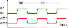
(a) synchronous setting

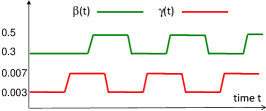
(b) asynchronous setting

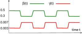
(c) anti-synchronous setting

Figure 2: Examples of synchronous, asynchronous, and counter-synchronous $\beta(t)$ and $\gamma(t)$

Figure 3 plots the curves obtained by simulation and by model computing in the case of both $\beta_{v}(t)$ and $\gamma_{v}(t)$ have period $T=8$ and $T=16$ (as shown in Figure 2). In each graph, we let the virus initially infect 2,292 or 20% vertices that are randomly selected; note that the degree of initial infection does not impact whether the virus spreading will die out or not. Since the model computing and simulation results (obtained as the average of 50 simulation runs) match almost perfectly no matter the virus spreading will die out or not, we will use simulation and model computing interchangeably. Since the same phenomenon applies to both cases of $T=8$ and $T=16$, in what follows we only report the case of $T=8$. Again, the accuracy result allows us to obtain $i_{v}(t)$ via model computing in the process of confirming the analytical results of our adaptive control strategies.

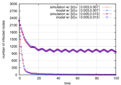
(a) T=8

(b) T=16

Figure 3: Model accuracy

3.2 Confirmation of the sufficient conditions in the semi-adaptive scenario

In this section, we use the aforementioned Oregon graph to confirm our analytical results presented in Section 2.2. We confirm Theorem 2.3 and Corollary 2.5 because they offer succinct sufficient conditions under which the virus spreading dies out.

3.2.1 Confirmation of Theorem 2.3

For the graph, we let the virus initially infect 2,292 or 20% randomly selected nodes, and consider three cases between the model’s input parameter — synchrony, asynchrony, and anti-synchrony as illustrated in Figure 2. Since Theorem 2.3 has two parts, we confirm them respectively.

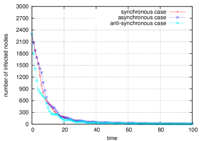
(a) Parameter set (i)

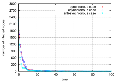
(b) Parameter set (ii)

Figure 4: Confirmation of sufficient condition under which virus spreading dies out ($T=8$)

Case 1: Confirmation of the sufficient condition under which the virus spreading will die out. We consider two sets of parameters: (i) $\beta(t)\in\{0.3,0.5\}$ and $\gamma(t)\in\{0.003,0.007\}$; (ii) $\beta(t)\in\{0.1,0.22\}$ and $\gamma(t)\in\{0.001,0.003\}$. Both functions, $\beta(t)$ and $\gamma(t)$, have period $T=8$. Both parameter sets satisfy the sufficient condition of Theorem 2.3, namely $\lambda_{1}<\bar{\beta}/\bar{\gamma}$, which means that the virus spreading will die out. Figure 4 plots the dynamics of the numbers of infected nodes with respect to time. From Figure 4 we can draw the following observations. First, the virus spreading does die out at about the 50th and 25th step, respectively, which confirms the sufficient condition under which the virus spreading will die out. It is an interesting future work to quantitatively characterize how the speed of convergence (i.e., dying out) depends upon functions $\beta(t)$ and $\gamma(t)$. Second, it is counter-intuitive and interesting that the virus spreading is somewhat more effectively defended against in the anti-synchronous case than in the synchronous case, which is in turn more effectively defended against than in the asynchronous case. More studies are needed in order to explain this phenomenon. Third, the curves are convex, meaning that cure is more effective in the early stage of the attack-defense dynamics than in the later stage. For example, it takes a shorter period of time to reduce the infection from 2,292 nodes to 100 nodes than to reduce the infection from 100 nodes to zero nodes (i.e., dying out).

Case 2: Confirmation of the condition under which the virus spreading may not die out. We consider two sets of parameters: (i) $\beta(t)\in\{0.2,0.4\}$ and $\gamma(t)\in\{0.003,0.007\}$; (ii) $\beta(t)\in\{0.05,0.15\}$ and $\gamma(t)\in\{0.001,0.003\}$. Both functions, $\beta(t)$ and $\gamma(t)$, have period $T=8$. Both parameter sets do not satisfy the sufficient condition of Theorem 2.3 because $\lambda_{1}>\bar{\beta}/\bar{\gamma}$, which means that the virus spreading does not die out in some initial infection configurations.

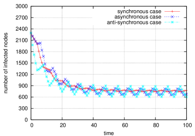
(a) Parameter set (i)

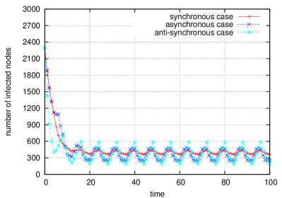
(b) Parameter set (ii)

Figure 5: Confirmation of virus spreading not dying out ($T=8$)

Figure 5 plots the dynamics, from which we draw the following observations. First, the virus spreading does not die out, which confirms Theorem 2.3. Second, all the curves exhibit periodic behaviors, but the extent of oscillation in the case of anti-synchrony is more significant than in the case of asynchrony, which in turn is more significant than in the case of synchrony. This means that the degree of synchrony between $\beta(t)$ and $\gamma(t)$ will impact the outcome when the virus spreading does not die out. Third, comparing Figures 5(a) and 5(b), we observe that, under the same synchrony, the outcome will depend on functions $\beta(t)$ and $\gamma(t)$. More studies are needed to characterize these dependence relationships.

3.2.2 Confirmation of Corollary 2.5

Corollary 2.5 gives an even more succinct sufficient condition under which the virus spreading will die out. For the graph, we let the virus initially infect 2,291 or 20% randomly selected nodes. For the case the sufficient condition in Corollary 2.5 is satisfied, we consider two sets of parameters that are uniformly chosen at random from certain intervals: (i) $\beta(t)\in[0.7,0.9]$ and $\gamma(t)\in[0.006,0.0014]$; (ii) $\beta(t)\in[0.1,0.3]$ and $\gamma(t)\in[0.0015,0.0035]$. In each parameter setting, the sufficient condition stated in Corollary 2.5 is satisfied, namely $\lambda_{1}<{\sf E}(\beta(0))/{\sf E}(\gamma(0))$, which means that the virus spreading will die out.

For the case the sufficient condition in Corollary 2.5 is not satisfied, we consider two sets of parameters that are uniformly chosen at random from certain intervals: (i) $\beta(t)\in[0.4,0.6]$ and $\gamma(t)\in[0.006,0.014]$; (ii) $\beta(t)\in[0.05,0.15]$ and $\gamma(t)\in[0.0015,0.0035]$. In each parameter setting, the sufficient condition stated in Corollary 2.5 is not satisfied because $\lambda_{1}>{\sf E}(\beta(0))/{\sf E}(\gamma(0))$, and thus the analytical result says that the virus spreading does not die out in some initial infection configurations.

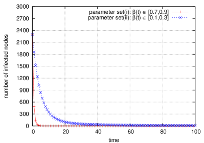
(a) The sufficient condition is satisfied

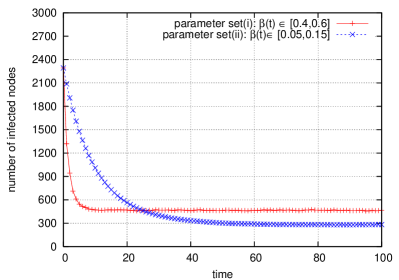
(b) The sufficient condition is not satisfied

Figure 6: Confirmation of Corollary 2.5 ($T=8$)

Figure 6(a) plots the dynamics of the number of infected nodes with respect to time when the sufficient condition is satisfied. From it we can draw the following observations. First, the virus spreading does die out, as predicted by Corollary 2.5. Second, the larger the $\beta(t)$, the more effective the defense against the virus spreading. Third, all the curves are convex, meaning that it takes a shorter period of time to significantly reduce the number of infected nodes (e.g., from 2,291 to 50) than to making the virus spreading die out (e.g., from 50 to zero).

Figure 6(b) plots the dynamics of the number of infected nodes with respect to time when the sufficient condition is not satisfied. From it we can draw the following observations. First, the virus spreading does not die out, which confirms Corollary 2.5. Second, the larger (in a stochastic sense) the $\beta(t)$, the earlier the system will converge to the steady state. However, the ultimate degree of infection does not depend on $\beta(t)$, but rather on ${\sf E}(\beta(0))/{\sf E}(\gamma(0))$, which means that ${\sf E}(\beta(0))/{\sf E}(\gamma(0))$ may be used as an indicator of steady-state infection when the virus spreading does not die out. It is an interesting future work to rigorously characterize this phenomenon.

3.3 Confirmation of the controllability in the fully-adaptive scenario

3.3.1 Confirmation of Theorem 2.6

Theorem 2.6 states that even if we do not know $\gamma(t)$ but we may be able to observe $i_{v}(t)$ and may be able to adjust the defense as needed, following its control strategy will cause the dying out of the virus spreading. To compare the effects of adaptive control and semi-adaptive control, in our simulation study, we also used the periodical functions $\beta(t)\in\{0.375,0.40\}$ and $\gamma(t)\in\{0.003,0.007\}$ with period $T=8$ as illustrated in Figure 2. These parameters satisfy the sufficient condition in Theorem 2.3, which means that the virus spreading will die out as we discussed above. To ensure comparability, we also let the virus initially infect 2,291 or 20% randomly selected nodes. As mentioned before, since the anti-synchronous defense is somewhat more effective than the synchronous and asynchronous defenses, we will compare it with the outcome of the adaptive control strategy.

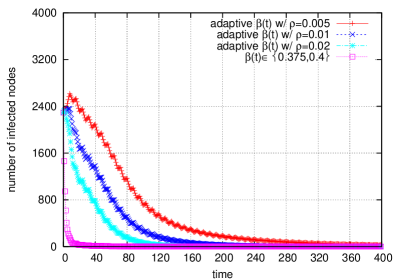
(a) Fully-adaptive control

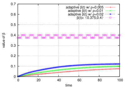
(b) Comparison of cure capabilities

Figure 7: Confirmation of semi-adaptive dying out vs. fully-adaptive control

Figure 7(a) plots the dynamics of the number of infected nodes with respect to time in the following four cases: the adaptive control parameter $\rho=0.005$; the adaptive control parameter $\rho=0.01$; the adaptive control parameter $\rho=0.02$; the comparison dynamics corresponding to the anti-synchronous case with $T=8$ periodical function $\beta(t)\in\{0.375,0.40\}$. We draw the following observations. First, $\rho$ plays a crucial role in indicating the rate at which the virus spreading dies out. For example, for $\rho=0.02$, it takes only about 80 steps to reduce the number of infected nodes from 2,291 to 160 (nevertheless it takes another 60 steps to kill the virus spreading, namely to reduce the number of infected nodes from 160 to zero); for $\rho=0.01$, it takes about 130 steps to reduce the number of infected nodes from 2,291 to 160 (nevertheless it takes about another 100 steps to kill the virus spreading, namely to reduce the number of infected nodes from 160 to zero). This also confirms the physical meanings of Proposition 2.8 discussed above.

Second, Figure 7(a) indicates that for all $\rho=0.005$, $\rho=0.01$ and $\rho=0.02$, the fully-adaptive defenses are less effective than the semi-adaptive defense represented by $\beta(t)\in\{0.375,0.40\}$. As we show in Figure 7(b), this is caused by the fact that the semi-adaptive $\beta(t)$ is much larger than the adaptive $\beta(t)$. This means that the sufficient condition in the semi-adaptive case, under which the virus spreading dies out, may be significantly beyond being necessary. In contrast, the fully-adaptive control strategy is much more “cost-effective” because larger $\beta(t)$ will likely cause a higher cost.

3.3.2 Confirmation of Theorem 2.10

Theorem 2.10 states that even if we do not know $\gamma(t)$ but we may be able to observe $i_{v}(t)$ and may be able to adjust the defense (but cannot kill the virus spreading), then following its control strategy will cause the containment of the virus spreading. In our simulation study, we used the periodical function $\gamma(t)\in\{0.0005,0.001\}$ with period $T=8$ similar to what was shown in Figure 2. This input parameter is not used in our adaptive control algorithm, rather it is merely for the purpose of comparison to the sufficient condition in Theorem 2.3, which requires the $\beta_{v}(t)$ satisfy certain property (for example, we use $\beta(t)\in\{0.01,0.02\}$, meaning that the virus spreading does not die out as predicated), and the $\beta_{v}(t)$ derived from our adaptive control strategy. To ensure the comparability, we also let the virus initially infect 2,291 or 20% randomly selected nodes. As mentioned before, since the anti-synchronous defense is more effective than the synchronous and asynchronous defenses, we will compare it with the outcome of the adaptive control algorithm.

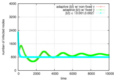
(a) Fully-adaptive control

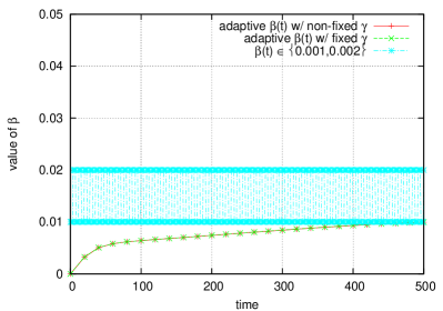
(b) Comparison of cure capabilities

Figure 8: Confirmation of the virus spreading containment via fully-adaptive control (the red-color curves are hidden behind the green-color curves)

In our simulation we set $i^{*}=0.1$ (i.e., we want to contain the degree of infection to 10%) and $u_{v}=0$ (i.e., a special case of Theorem 2.10). Figure 8(a) plots the dynamics of the number of infected nodes with respect to time in the following three cases: the adaptive control parameter $\rho=0.001$; the adaptive control parameter $\rho=0.001$ with fixed $\bar{\gamma}(t)=(0.0005+0.001)/2=0.00075$ as specified in Theorem 2.10); the comparison dynamics corresponding to the anti-synchronous case with $T=8$ periodical function $\beta(t)\in\{0.01,0.02\}$. We draw the following observations. First, the control strategy does contain the infection to the pre-determined level of $i^{*}=0.1$ or 10% infection. Moreover, the adaptive control strategy is robust because perturbation in $\gamma$ does not fundamentally change the dynamics behavior. This also confirms the physical meanings of Proposition 2.12 discussed above.

Second, Figure 8(a) indicates that the adaptive defenses are slightly less effective in defending against the virus spreading than the defense of $T=8$ periodical function $\beta(t)\in\{0.01,0.02\}$. As we show in Figure 8(b), the adaptive control strategy can be much more “cost-effective” because it leads to significantly smaller $\beta(t)$.

4 Conclusion

We have presented a novel dynamical systems model for studying both semi-adaptive and fully-adaptive defenses against virus spreading. For semi-adaptive defense, we give general as well as succinct sufficient conditions under which the virus spreading will die out. For fully-adaptive defense, we characterize two adaptive control strategies under which the virus spreading will die out or will be contained to a desired level of infection. Our analytical results are confirmed with simulation study.

This paper brings a range of open questions for future research. In addition to those mentioned in the body of the paper, here are more examples: What are the necessary conditions under which the virus spreading will die out? What are the optimal adaptive control strategies?

Acknowledgement. We thank the anonymous reviewers for their useful comments, and Raj Boppana for helpful discussion on the simulation.

This work was supported in part by AFOSR, AFOSR MURI, ONR, and UTSA. The views and conclusions contained in the article are those of the authors and should not be interpreted as, in any sense, the official policies or endorsements of the government or the agencies.

References

- Anderson and May (1991) Anderson, R. and May, R. 1991. Infectious Diseases of Humans. Oxford University Press.
- Arnold (1998) Arnold, L. 1998. Random Dynamical Systems. Springer-Verlag.
- Bailey (1975) Bailey, N. 1975. The Mathematical Theory of Infectious Diseases and Its Applications. 2nd Edition. Griffin, London.
- Berman and Shaked-Monderer (2003) Berman, A. and Shaked-Monderer, N. 2003. Completely positive matrices. World Scientific Publishing.
- Bhargava et al. (1986) Bhargava, B., Dilley, J., and Riedl, J. 1986. Raid: a robust and adaptable distributed system. In ACM SIGOPS European Workshop.
- Chakrabarti et al. (2008) Chakrabarti, D., Wang, Y., Wang, C., Leskovec, J., and Faloutsos, C. 2008. Epidemic thresholds in real networks. ACM Trans. Inf. Syst. Secur. 10, 4, 1–26.
- Ganesh et al. (2005) Ganesh, A., Massoulie, L., and Towsley, D. 2005. The effect of network topology on the spread of epidemics. In Proceedings of IEEE Infocom 2005.
- Hethcote (2000) Hethcote, H. 2000. The mathematics of infectious diseases. SIAM Rev. 42, 4, 599–653.
- Kephart and White (1991) Kephart, J. and White, S. 1991. Directed-graph epidemiological models of computer viruses. In IEEE Symposium on Security and Privacy. 343–361.
- Kephart and White (1993) Kephart, J. and White, S. 1993. Measuring and modeling computer virus prevalence. In IEEE Symposium on Security and Privacy. 2–15.
- Kermack and McKendrick (1927) Kermack, W. and McKendrick, A. 1927. A contribution to the mathematical theory of epidemics. Proc. of Roy. Soc. Lond. A 115, 700–721.
- LaSalle (1960) LaSalle, J. 1960. Some extensions of liapunov’s second method. IRE Trans. Circuit Theory 7, 520–527.
- McKendrick (1926) McKendrick, A. 1926. Applications of mathematics to medical problems. Proc. of Edin. Math. Soceity 14, 98–130.
- Oseledec (1968) Oseledec, V. 1968. A multiplicative ergodic theorem. characteristic ljapunov, exponents of dynamical systems. English Translation. Trans. Moscow Math. Soc. 19, 197–231.
- Pesin (1977) Pesin, Y. B. 1977. Characteristic lyapunov exponents and smooth ergodic theory. Russ. Math. Surv. 32, 55–114.
- Wang et al. (2003) Wang, Y., Chakrabarti, D., Wang, C., and Faloutsos, C. 2003. Epidemic spreading in real networks: An eigenvalue viewpoint. In Proc. of the 22nd IEEE Symposium on Reliable Distributed Systems (SRDS’03). 25–34.
- Zou et al. (2005) Zou, C., Duffield, N., Towsley, D., and Gong, W. 2005. Adaptive defense against various network attacks. In Workshop on Steps to Reducing Unwanted Traffic on the Internet (SRUTI’05). 69–75.