Abstract

The twist free energy is computed in the Villain formulation of the $3D$ $U(1)$ lattice gauge theory at finite temperature. This enables us to obtain renormalization group equations describing a critical behavior of the model in the vicinity of the deconfinement phase transition. These equations are used to check the validity of the Svetitsky-Yaffe conjecture regarding the critical behavior of the lattice $U(1)$ model. In particular, we calculate the two-point correlation function of the Polyakov loops and determine some critical indices.

1 Introduction

The critical behavior of pure lattice gauge theories (LGTs) at finite temperatures is well understood for non-abelian $SU(N)$ theories in various dimensions. In particular, the phase structure of a finite-temperature three-dimensional ($3D$) pure $SU(N)$ LGT with the standard Wilson action is thoroughly investigated both for $N=2,3$ and for the large-$N$ limit (see, e.g., [1] and references therein). The transition is second order for $N=2,3$ and first order for $N>4$. In the case of the $SU(4)$ gauge group, most works agree that the transition is weakly first order. The deconfining transition in $SU(N=2,3)$ LGTs belongs to the universality class of $2D$ $Z(N=2,3)$ Potts models. All these phase transitions are characterized by the spontaneous symmetry breaking of a $Z(N)$ global symmetry of the lattice action in the high-temperature deconfining phase.

Surprisingly, the situation is much less clear for the $3D$ $U(1)$ LGT. The present state of affairs can be briefly summarized as follows. $3D$ theory was studied by Parga using Lagrangian formulation of the theory [2]. At high temperatures the system becomes effectively two-dimensional, in particular the monopoles of the original $U(1)$ gauge theory become vortices of the $2D$ system. The partition function turns out to coincide (in the leading order of the high-temperature expansion) with the $2D$ $XY$ model in the Villain representation. The $XY$ model is known to have the Berezinskii-Kosterlitz-Thouless (BKT) phase transition of the infinite order [3, 4]. According to the Svetitsky-Yaffe conjecture the finite-temperature phase transition in the $3D$ $U(1)$ LGT should belong to the universality class of the $2D$ XY model [5]. This means, firstly that the global $U(1)$ symmetry cannot be broken spontaneously because of the Mermin-Wagner theorem [6] and, consequently the local order parameter does not exist for this type of the phase transition. Secondly, the correlation function of the Polyakov loops (which become spins of the $XY$ model) decreases with the power law at $\beta\geq\beta_{c}$ implying a logarithmic potential between heavy electrons

$$P(R)\ \asymp\ \frac{1}{R^{\eta(T)}}\ ,$$ (1)

where the $R\gg 1$ is the distance between test charges. The critical index $\eta(T)$ is known from the renormalization-group analysis of Ref.[4] and equals $\eta(T_{c})=1/4$ at the critical point of the BKT transition. For $\beta<\beta_{c}$, $t=\beta_{c}/\beta-1$ one has

$$P(R)\ \asymp\ \exp\left[-R/\xi(t)\right]\ ,$$ (2)

where the correlation length $\xi\sim e^{bt^{-\nu}}$ and the critical index $\nu=1/2$. Therefore, the critical indices $\eta$ and $\nu$ should be the same in the finite-temperature $U(1)$ model if the Svetitsky-Yaffe conjecture holds in this case. The first numerical check of these predictions was performed on the lattices $L^{2}\times N_{t}$ with $L=16,32$ and $N_{t}=4,6,8$ in [7]. Though authors of [7] confirm the expected BKT nature of the phase transition, the reported critical index is almost three times larger of that predicted for the $XY$ model, $\eta\approx 0.78$. More recent analytical and numerical studies of Ref.[8] indicate that at least on the anisotropic lattice in the limit of vanishing spatial coupling $\beta_{s}$ (where space-like plaquettes are decoupled) the $3D$ $U(1)$ gauge model exhibits the critical behavior similar to the $XY$ spin model. However, numerical simulations of the isotropic model on the lattices up to $L=256$ and $N_{t}=8$ reveal that $\eta\approx 0.49$, i.e. still far from the $XY$ value [9]. Thus, so far there is no numerical indications that critical indices of $3D$ $U(1)$ LGT coincide with those of the $2D$ $XY$ model and the question of the universality remains open if $\beta_{s}$ is non-vanishing.

On the analytical side one should mention a renormalization group (RG) study of Refs.[5, 10]. In both cases a high-temperature and a dilute monopole gas approximations were used for the Villain formulation which helped to derive an effective sine-Gordon model. Resulting RG equations were shown to converge rapidly with iterations to RG equations of the $2D$ $XY$ model. It gives a strong indication that, indeed the nature of the phase transitions in both models is the same. Moreover, since the scaling of the lattice spacing coincides in both cases the critical index $\nu$ should also be the same (this however was not proven). Furthermore, neither critical points nor index $\eta$ has been determined in previous studies.

In this work we re-examine the critical behavior of the Villain formulation of the $3D$ $U(1)$ LGT aiming to compute both critical indices $\nu$ and $\eta$ as well as to determine the location of the critical points. In order to achieve this goal we calculate the free energy of the model in the presence of a twist and express it like a function of a bare coupling, a monopole activity and adimensional ratio of the anisotropic couplings. Varying the lattice cut-off one then finds the RG equations in a standard manner. We analyze the equations thus obtained for different values of $N_{t}$. Also, we present results for the correlation function of the Polyakov loops which allow to extract the index $\eta$ at the critical point.

2 Definition of the model and its dual

We work on a periodic $3D$ lattice $\Lambda=L^{2}\times N_{t}$ with spatial extension $L$ and temporal extension $N_{t}$. We introduce anisotropic dimensionless couplings as

$$\beta_{t}=\frac{1}{g^{2}a_{t}}\ ,\;\;\;\;\;\beta_{s}=\frac{\xi}{g^{2}a_{s}}\ =\ \beta_{t}\ \xi^{2}\ ,\;\;\;\;\;\xi=\frac{a_{t}}{a_{s}}\ ,$$ (3)

where $a_{t}$ ($a_{s}$) is lattice spacing in the time (space) direction, $g^{2}$ is the continuum coupling constant with dimension $a^{-1}$. $\beta=a_{t}N_{t}$ is an inverse temperature.

The compact $3D$ $U(1)$ LGT on the anisotropic lattice in the presence of the twist is defined through its partition function as

$$Z(\beta_{t},\beta_{s})=\int_{0}^{2\pi}\prod_{x\in\Lambda}\>\prod_{n=1}^{3}\frac{d\omega_{n}(x)}{2\pi}\ \exp{S[\omega+\theta]}\ ,$$ (4)

where $S$ is the Wilson action

$$S[\omega] = \beta_{s}\sum_{p_{s}}\cos\omega(p_{s})+\beta_{t}\sum_{p_{t}}\cos\omega(p_{t})\ ,$$ (5)

$$\omega(p)\ = \ \omega_{n}(x)\ +\ \omega_{m}(x+e_{n})\ -\ \omega_{n}(x+e_{m})\ -\ \omega_{m}(x)\$$ (6)

and sums run over all space-like ($p_{s}$) and time-like ($p_{t}$) plaquettes. We take a constant shift $\theta_{n}$ on a stack of plaquettes wrapping around the lattice in the spatial directions, e.g. the shift $\theta_{1}$ on the plaquettes with coordinates $p=(n_{2},n_{3};x_{1},0,0)$ and the shift $\theta_{2}$ on the plaquettes with coordinates $p=(n_{1},n_{3};0,x_{2},0)$ (for a detailed description of the twist in LGT we refer the reader to Ref. [11] where also some properties of the twisted partition function are discussed).

In order to calculate the free energy in the presence of the twist we make the following quite standard steps:

• Perform duality transformations with the twisted partition function;

• Replace the dual Boltzmann weight with the Villain formulation and calculate an effective monopole theory;

• Sum up over monopole configurations in the dilute gas approximation.

All these steps are well known in the context of the $3D$ $U(1)$ LGT and can be easily generalized for the anisotropic lattice in the presence of the twist. For the duality transformations we need an approach of Ref. [12] which takes correctly into account the periodic boundary conditions on the abelian gauge fields. For the anisotropic theory with twist we find

$$Z(\theta_{n})\ =\ \sum_{h_{n}=-\infty}^{\infty}e^{i\sum_{n=1}^{2}\ h_{n}\theta_{n}}\ Z(h_{n})\ ,$$ (7)

where the global summation over $h_{n}$ enforces the global Bianchi constraint on the periodic system and $Z(h_{n})$ is the dual partition function

$$Z(h_{n})\ =\ \sum_{r(x)=-\infty}^{\infty}\ \prod_{x}\ \prod_{n=1}^{3}\ I_{r(x)-r(x+e_{n})+\eta_{n}(x)}(\beta_{n})\ .$$ (8)

Here $I_{r}(x)$ is the modified Bessel function and we have introduced sources $\eta_{n}(x)=\eta(l)$ as

$$\eta(l)\ =\ \begin{cases}h_{n},&l\in P_{d}\ ,\\ 0,&\text{otherwise}\ ,\end{cases}$$ (9)

where $P_{d}$ is a set of links dual to twisted plaquettes (this set forms a closed loop on the dual lattice), $\beta_{n}=\beta_{s},n=3$ and $\beta_{n}=\beta_{t},n=1,2$. In the limit $\beta_{s}=0$ and in the absence of the twist the partition function (7) reduces to ($x=(x_{1},x_{2})$ runs now over two-dimensional lattice $L^{2}$)

$$Z(0)\ =\ \sum_{r(x)=-\infty}^{\infty}\ \prod_{x}\ \prod_{n=1}^{2}\ I_{r(x)-r(x+e_{n})}^{N_{t}}(\beta_{n})\ .$$ (10)

In this limit the model becomes a generalized version of the $XY$ model, and it was studied both analytically and by Monte-Carlo simulations in Ref.[8]. The firm conclusion of Ref.[8] was that the model (10) is in the same universality class as the $XY$ model. Here we are going to study an opposite limit, namely $\beta_{t}>\beta_{s}\gg 1$ which lies close to the continuum limit of the full $3D$ $U(1)$ model. When both couplings are large it is customary to use the Villain approximation, i.e.

$$I_{r}(x)/I_{0}(x)\ \approx\ \exp\left(-\frac{1}{2x}r^{2}\right)\ .$$ (11)

This dual form of the twisted partition function, Eqs. (7)-(11), is a starting point of the analysis in the next Sections.

3 Free energy of a twist

Substituting (11) into the partition function (8) we use the Poisson summation formula to perform summation over $r(x)$ variables. The partition function is factorized in the product of the dual massless photon contribution and the contribution from the monopole configurations

$$Z(h_{n})\ =\ Z_{ph}\ Z_{m}\ .$$ (12)

Taking into account the definition (9) and performing summation over the lattice we write these contributions in the presence of the twist as

$$Z_{ph}\ =\ \exp\left[-\frac{N_{t}}{2\beta_{t}}\left(h_{1}^{2}+h_{2}^{2}\right)\right]\ ,$$ (13)

$$Z_{m}\ =\ \sum_{\{m_{x}\}}\exp\left[-\pi^{2}\sum_{x,x^{\prime}}m_{x}G_{xx^{\prime}}m_{x^{\prime}}-\frac{2\pi i}{L}\sum_{x}m_{x}\left(h_{1}x_{1}+h_{2}x_{2}\right)\right]\;.$$ (14)

Here, $G_{xx^{\prime}}$ is the three-dimensional Green function on anisotropic lattice. For our purposes it is convenient to present it in the form ($x_{3}=t$)

$$G_{x,t;x^{\prime},t^{\prime}}\ =\ \frac{\beta_{t}}{N_{t}}\left(G_{x,x^{\prime}}^{2d}+\sum_{k=1}^{N_{t}-1}e^{\frac{2\pi i}{N_{t}}k(t-t^{\prime})}G_{x,x^{\prime}}^{2d}(M_{k})\right)\ ,$$ (15)

where $G_{x}^{2d}$ is massless and $G_{x}^{2d}(M_{k})$ massive $2D$ Green function with a mass

$$M_{k}^{2}\ =\ \beta_{t}/\beta_{s}(1-\cos 2\pi k/N_{t})\;.$$ (16)

Since massive Green functions are exponentially suppressed for $x\neq x^{\prime}$ near the continuum limit like $\exp(-M_{k}R)$ we keep in the sum over temporal momenta $k$ in (15) only the terms with smallest $M_{k}$, corresponding to $k=1,N_{t}-1$. Introducing notations $m_{x}=\sum_{t=0}^{N_{t}-1}m_{x,t}$, $r_{x}^{k}=\sum_{t=0}^{N_{t}-1}m_{x,t}\exp\frac{2\pi ikt}{N_{t}}$ and keeping only leading contribution in the Taylor expansion of the terms with $x\neq x^{\prime}$ we bring $Z_{m}$ to the following form

$$Z_{m}=\sum_{\{m_{x,t}\}}\exp-\frac{\pi^{2}\beta_{t}}{N_{t}}\left(\sum_{x,x^{\prime}}m_{x}G_{xx^{\prime}}^{2d}m_{x^{\prime}}+\sum_{k=1}^{N_{t}-1}\sum_{x}r_{x}^{k}G_{0}^{2d}(M_{k})r_{x}^{-k}\right)$$

$$\prod_{x\neq x^{\prime}}\left(1-\frac{2\pi^{2}\beta_{t}}{N_{t}}r_{x}^{1}G_{xx^{\prime}}^{2d}(M_{1})r_{x^{\prime}}^{-1}\right)\exp\left[-\frac{2\pi i}{L}\sum_{x}m_{x}\left(h_{1}x_{1}+h_{2}x_{2}\right)\right]\;.$$ (17)

Consider a set of $m_{x,t}$ variables at one spatial $x$ position. Since all non-vanishing $r_{x}^{k}$ are suppressed by massive Green functions, the dominant contribution arises from the following configurations: 1) $m_{x}=0,r_{x}^{k}=0$; 2) $m_{x}=0$, $r_{x}^{k}=\pm\left(1-\exp\frac{2\pi ik}{N_{t}}\right)\exp\frac{2\pi ik\tau}{N_{t}}$; 3) $m_{x}=\pm 1$, $r_{x}^{k}=\pm\exp\frac{2\pi ik\tau}{N_{t}}$. Since $G_{x}^{2d}$ diverges logarithmically in the large-volume limit, only neutral configurations $\sum_{x}m_{x}=0$ contribute in this limit. If $\frac{\beta_{t}}{N_{t}}=T/g^{2}$ is large enough we can restrict ourselves only to leading contribution with $m_{z}=1$, $m_{z^{\prime}}=-1$ and sum over $(z,z^{\prime})$. Summing up over all these configurations we finally obtain after a long algebra

$$Z_{m}\ \approx\ \exp\left[L^{2}\ \sum_{z\neq 0}\exp\left[-\frac{2\pi^{2}\beta_{t}}{N_{t}}\ D(z)+\frac{2\pi i}{L}\left(h_{1}z_{1}+h_{2}z_{2}\right)\right]F(z)\right]\ .$$ (18)

The constant overall factor has been omitted. Here, $D(z)$ is the infrared-finite Green function whose asymptotics is given by $D(z)\ \asymp\ \frac{1}{\pi}\ \log(z_{1}^{2}+z_{2}^{2})^{1/2}+\frac{1}{2}$. If $F(z)=1$, the partition function (18) coincides with the vortex partition function of the $XY$ model in the presence of the twist. For the case of the finite-temperature $U(1)$ LGT the function $F(z)$ reads

$$F(z)\ =\ C_{1}+C_{2}\left(G_{z}^{2d}(M_{1})\right)^{2}\ .$$ (19)

It incorporates two new contributions. The constant contribution

$$C_{1}\ =\ \left(\frac{N_{t}W_{0}}{1+2N_{t}W_{1}}\right)^{2}\ \left(1+\frac{16\pi^{4}\beta_{t}^{2}}{N_{t}^{2}}U(1-U)\sum_{x\neq 0}\left(G_{x}^{2d}(M_{1})\right)^{2}\right)$$ (20)

renormalizes a monopole activity while the second one proportional to $C_{2}$

$$C_{2}\ =\ \frac{8\pi^{4}\beta_{t}^{2}}{N_{t}^{2}}\ \left(\frac{N_{t}W_{0}}{1+2N_{t}W_{1}}\right)^{2}\ (1-U)^{2}\ ,$$ (21)

gives an additional renormalization for the monopole-antimonopole logarithmic interaction at high temperatures. The constants introduced in the above equations are given by

$$U = 2(1-\cos\frac{2\pi}{N_{t}})\left(\frac{2N_{t}W_{1}}{1+2N_{t}W_{1}}\right)\;,$$

$$W_{m} = \exp\left[-\frac{\pi^{2}\beta_{t}}{N_{t}}\sum_{k=1}^{N_{t}-1}\left(2-m-\cos\frac{2\pi k}{N_{t}}m\right)G_{0}^{2d}(M_{k})\right],m=0,1\;.$$

Noting that both $D(z)$ and $F(z)$ depend only on $r=(z_{1}^{2}+z_{2}^{2})^{1/2}$ we can factorize the angular dependence of the twist. Integrating over the polar angle and replacing the summation over $r$ with integration near the continuum limit we find for the exponent of Eq. (18)

$$L^{2}\ \int_{1}^{+\infty}\exp\left[-\frac{2\pi^{2}\beta_{t}}{N_{t}}\ D(r)\right]F(r)\ J_{0}\left(\frac{2\pi i}{L}r\right)dr\ ,$$ (22)

where $J_{0}(x)$ is the Bessel function. Combining this result with Eq. (13) and summing up over $h_{n}$ in Eq. (7) gives us the following expression for the twisted partition function in the thermodynamic limit

$$Z(\theta)\ =\ \sum_{n_{i}=-\infty}^{+\infty}\exp{\left(-\frac{\beta_{eff}}{2}\sum_{i=1,2}(\theta_{i}-2\pi n_{i})^{2}\right)}\ .$$ (23)

We have introduced here the renormalized coupling constant $\beta_{eff}$

$$\frac{1}{\beta_{eff}}\ =\ \frac{N_{t}}{\beta_{t}}+2\pi^{3}y^{2}\int_{1}^{+\infty}r^{3-2\pi\frac{\beta_{t}}{N_{t}}}\left(1+\frac{C_{2}}{C_{1}}\ \left(G_{r}^{2d}(M_{1})\right)^{2}\right)dr\ .$$ (24)

The first term corresponds to the massless photon contribution while the second one arises due to monopole-antimonopole interaction. The monopole activity $y$ is given by

$$y\ =\ 2\ C_{1}^{1/2}\exp\left({-\frac{1}{2}\pi^{2}\frac{\beta_{t}}{N_{t}}}\right)\ .$$ (25)

Following the same strategy one can compute the two-point correlation function of the Polyakov loops in the representation $j$ which appears to have a power-like decay of the form

$$P_{j}(R)\ \approx\ \exp\left[-\frac{j^{2}}{2\pi\beta_{eff}}\ \ln R\right]\ .$$ (26)

4 The renormalization group equations

The RG equations can be derived from the expression for $\beta_{eff}$ by integrating in Eq. (24) between length scales $a$ and $a+\delta a$, see e.g [13]. Renormalizing masses $M_{k}$ in such a way to preserve $G_{r}^{2d}(M_{k})$ we obtain RG equations in a differential form as ($t=\ln a$)

$$\frac{d\beta_{t}}{dt} = -2\pi^{3}y^{2}\frac{\beta_{t}^{2}}{N_{t}}\left(1+\frac{C_{2}}{C_{1}}\ \left(G_{1}^{2d}(M_{1})\right)^{2}\right)\ ,$$

$$\frac{dy}{dt} = y\;\left(2-\pi\frac{\beta_{t}}{N_{t}}\right)\ ,\ \frac{dM_{k}}{dt}=M_{k}\ .$$ (27)

When $N_{t}=1$ these equations are reduced to the equations of the $2D$ $XY$ model. The equations for $M_{k}$ can be solved explicitly $M_{k}(t)=M_{k}(0)e^{t}$. Thus, $M_{k}$ grows exponentially with $t$ and in the limit $M_{k}\to\infty$ we again obtain RG equations of the $2D$ $XY$ model. Hence, we can expect that the critical indices of the model that describe the solution around a fixed point coincide with those of the $2D$ $XY$ model. To check that this is the case we solve the equations (27) numerically in the vicinity of the fixed point $\beta_{t}=2N_{t}/\pi,\ y=0$.

Fixing $\beta_{s}/\beta_{t}$ gives us an initial value for $M_{k}$. It should be sufficiently large to ensure the fast convergence of the Taylor expansion in Eq. (17). We have studied several initial values and have found no difference in the final result. As an example, in the Fig. 1 we compare the renormalization flow for $N_{t}=1$ ($2D$ $XY$ model) with that of $N_{t}=8$ taken $M_{1}=4$ as the initial value. The critical index $\nu$ can be obtained from fitting the values of the cut-off $a$ at which $\beta_{t}(a)$ flows to the fixed point $2N_{t}/\pi$ from above (massive phase). As a fitting function we use $a\sim\exp A(\beta_{t}-\beta_{t,\rm crit})^{-\nu}$. Our results for the critical points and $\nu$ values are summarized in the Table 1. We observe that for all $N_{t}$ the value of $\nu$ is compatible with the $XY$ value $\nu=1/2$. The critical index $\eta$ can also be determined at the fixed point. Since $\beta_{eff}(\beta_{t,\rm crit})=2/\pi$ we find from Eq. (26) $\eta=1/4$ for $j=1$.

To construct the continuum limit we fitted the critical couplings $\beta_{t,\rm crit}$ using several dependence on $N_{t}$. The best result is obtained with the fitting function $\beta_{t,\rm crit}=0.139+0.661N_{t}$. Thus, in the continuum limit the critical point is defined by $T_{c}\approx 0.661g^{2}$. The Fig. 2 shows the fitting function together with values of $\beta_{t,\rm crit}$ from the Table 1.

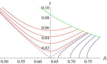
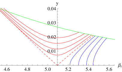
Figure 1: Renormalization flow for $N_{t}=1$ (left) and $N_{t}=8$ (right) obtained from numerical solution of RG equations. Green line defines the initial points, dashed red line is the critical line, blue lines show RG flow in the massless phase ($\beta>\beta_{t,\rm crit}$), red lines show RG flow in the massive phase ($\beta<\beta_{t,\rm crit}$).

$N_{t}$	$\beta_{t,\rm crit}$	$\nu$
1	0.748	0.498
2	1.447	0.499
4	2.785	0.506
6	4.122	0.503
8	5.445	0.503
12	8.082	0.504
16	10.718	0.504

Table 1: Values of $\beta_{t,\rm crit}$ and $\nu$ obtained for various $N_{t}$.

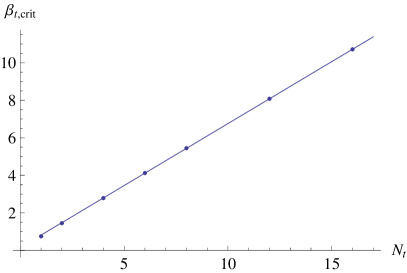
Figure 2: Critical points for $N_{t}=1,2,4,6,8,12,16$ fitted with the line $\beta_{t,\rm crit}=0.139+0.661N_{t}$.

5 Summary

In this paper we have computed the twist free energy of the finite-temperature $3D$ $U(1)$ LGT in the Villain formulation. This enabled us to obtain and analyze the RG equations which describe the critical behavior of the model across the deconfinement phase transition. Our main findings can be shortly summarized as follows.

• We have computed the critical points for various temporal extension $N_{t}$. In the continuum limit we find $T_{c}\approx 0.661g^{2}$.

• The scaling of the correlation length $\xi\sim a$ is compatible with a phase transition of the infinite order. Moreover, the critical index $\nu\approx 1/2$.

• We have also derived the leading asymptotic behavior of the Polyakov loop correlation function. This allowed us to determine the critical index $\eta$ at the critical point $\eta(\beta_{t,\rm crit})=1/4$.

This supports the Svetitsky-Yaffe conjecture that the deconfinement phase transition in the finite-temperature $3D$ $U(1)$ LGT belongs to the universality class of the $2D$ $XY$ model, at least in the region of bare coupling constants where our approximations hold, i.e. for $\beta_{t}/\beta_{s}>1$. For isotropic lattices, used in [9], the initial value becomes $\beta_{t}/\beta_{s}=1$. In this case one should take into account higher order terms of the Taylor expansion in the calculation of $Z_{m}$ which is hard to accomplish analytically. Still, we feel that the universality can be demonstrated also in this case by performing large-scale Monte-Carlo simulations of the isotropic model. Such computations are now in progress.

References

- [1] J. Liddle, M. Teper, arXiv:0803.2128 [hep-lat].
- [2] N. Parga, Phys.Lett. B107 (1981) 442.
- [3] V. Berezinskii, Sov.Phys. JETP 32 (1971) 493.
- [4] J. Kosterlitz, D. Thouless, J.Phys. C6 (1973) 1181; J. Kosterlitz, J.Phys. C7 (1974) 1046.
- [5] B. Svetitsky, L. Yaffe, Nucl.Phys. B210 (1982) 423.
- [6] N. Mermin, H. Wagner, Phys.Rev.Lett. 22 (1966) 1133.
- [7] P. Coddington, A. Hey, A. Middleton, J. Townsend, Phys.Lett. B175 (1986) 64.
- [8] O. Borisenko, M. Gravina, A. Papa, J. Stat. Mech. 0808 (2008) P08009.
- [9] O. Borisenko, R. Fiore, M. Gravina, A. Papa, J. Stat. Mech. 1004 (2010) P04015.
- [10] O. Borisenko, PoS LAT 2007, 170 (2007).
- [11] M. Vettorazzo, P. de Forcrand, Nucl. Phys. B686 (2004) 85.
- [12] G. Batrouni, M.B. Halpern, Phys. Rev. D30 (1984) 1782.
- [13] D. R. Nelson, J. Kosterlitz, Phys. Rev. Lett. 39 (1977) 1201.