Tunable Bound States in Continuum by Optical Frequency

Abstract

We demonstrate the existence of tunable bound-states in continuum (BIC) in a 1-dimensional quantum wire with two impurities induced by an intense monochromatic radiation field. We found that there is a new type of BIC due to the Fano interference between two optical transition channels, in addition to the ordinary BIC due to a geometrical interference between electron wave functions emitted by impurities. In both cases the BIC can be achieved by tuning the frequency of the radiation field.

I Introduction

The phenomenon of bound-states in continuum (BIC) was first discovered by Wigner and von Neumann Von -W (1). Subsequent studies can be found in a number of papers (e.g., Sudarshan (2)-Sadreev (7)). An experimental report showed evidence of BIC in super-lattice structures of quantum wells with a single impurity site F.Cappasso (8) or in single defect tube P. S. Deo (9). Examples of BIC in a double-cavity, 2-dimensional (2D) electron waveguide was reported in Ordonez-Na (10)-Linda (11).

In general if a discrete state embeds inside the continuum, the state will become unstable due to the resonance effect. If the transition channels are more than one, the resonance line-shape becomes asymmetric due to the quantum interference between those decay channels. The phenomenon often refereed as the Fano interference Fano (18, 19). There are many studies that have followed Fano’s work. However, the phenomena of the BIC and the Fano interference have been often studied as individual effects. In this paper we discuss the relation between BIC and Fano interference.

As an example, we consider here a tight-binding model with two intra-atoms attached to a semiconductor nanowire under a constant irradiation of an intense monochromatic radiation field. An electron of an intra-atom is excited by the radiation field from a lower energy state to an intermediate energy state to states with a continuous range of energies; alternatively, the electron from the lower energy state can jump directly to the continuous states. We label these two optical transition paths as $T_{1\cdot}$ and $T_{2\cdot}$, respectively (see FIG.1). Since there are two optical transition channels, Fano interference appears in this model

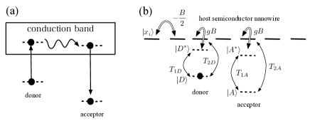
Figure 1: (a) Energy levels of donor and acceptor atoms. (b) Transitions among energy levels

The main results that we present in this paper are twofold: The first one is a new type of BIC in this system. In this BIC, the energy of the bound state depends on the coupling constant $g$ of the interaction between the discrete state and the continuum. This is not the case of ordinary BIC that has been discussed before (see, e.g., Refs. Tanaka (5, 6)). The ordinary BIC can be found for special values of energy of the discrete state that are imbedded in the continuum, where the energy shift of the discrete state due to the interaction vanishes. This value of the energy may found by requiring that the so-called “self-energy part”of the discrete state vanishes. Hence, this type of BIC has the same energy as the unperturbed energy without the interaction. We found this type of BIC in our model. In addition, however, we found the new type of BIC as mentioned above. Since this new type of BIC depends on the interaction, we call this a “dynamic BIC,” while we call the ordinary type of BIC a “static BIC.” As discussed in Tanaka (5), the static BIC is due to a geometrical interference in the wire between electron wave functions emitted by impurities. In contrast, the dynamic BIC appears because of the multichannels of the transition, $T_{1}{\cdot}$ and $T_{2}{\cdot}$, as we shall show. Hence, the dynamic BIC is the result of Fano interference.

The second main result is that because the freedom to chose the frequency of the radiation field, both BIC (the dynamic BIC and static BIC) may exist for wide value of the spectrum of the discrete state. This is not the case of the BIC that has been discussed in Tanaka (5) for the system without the radiation field. Indeed, in the absence of the radiation field, we have shown in Tanaka (5) that the BIC may exist only for a special value of the discrete energy. In contrast, here one can tune the frequency of the radiation field in order to achieve the BIC for arbitrary value of the energy of the discrete state. This tune-ability makes the BIC phenomena much more feasible to observe experimentally.

This paper is organized as follows. In section 2, we introduce the model. Then, we decompose the Hamiltonian of the system into the symmetric part and anti-symmetric part so that we can analyze our problem in much simpler form. In section 3, we construct the complex eigenvalue of resonance states to analyze the instability of the discrete states inside the continuum. Then we find the BIC by requiring that the imaginary part of the complex eigenvalue of the Hamiltonian vanishes at the BIC. In section 4, we present several cases of the dynamic BIC and the static BIC by plotting the imaginary part of the eigenvalue as a function of the frequency of the radiation field. In section 5, we summarize our results.

II Model

We shall consider a semiconductor nanowire with donor-acceptor impurities, e.g. 3D transition metal impurities Pradhan11 (14, 15), where the multiplet discrete levels of transition metals appear in the semiconductor band gap Watanabe87 (16). An electron of a donor is excited by an optical transition and is transferred to the acceptor through a semiconductor conduction band, and the electron is dexcited by an intra-atomic transition to emit a photon (see FIG. 1).

We show the model system of the present work in FIG. 1. The system consists of a semiconductor nanowire with donor and acceptor impurities located at $x_{D}$ and $x_{A}$, respectively. The semiconductor nanowire is described by a 1D tight-binding model with a nearest neighbor interaction $-B/2$ yielding a 1D conduction band with bandwidth $B$ with a lattice constant of $d$. We consider the lower and higher energy states of the donor (acceptor) impurity represented by $|D\rangle$ ($|A\rangle$) and $|D^{*}\rangle$ ($|A^{*}\rangle$), respectively. In this paper we use a conventional notation “*” for excited states used in Atomic Molecular and Optical physics. We consider the charge transfer between the higher energy state to the nanowire at the impurity sites of $x_{D}$ and $x_{A}$ with a coupling $gB$, where $g$ is a dimensionless coupling constant. The electronic Hamiltonian is then represented by

$$H_{el} = E_{D}|D\rangle\langle D|+E_{D^{*}}|D^{*}\rangle\langle D^{*}|$$ (1)

$$+E_{A}|A\rangle\langle A|+E_{A^{*}}|A^{*}\langle A^{*}|$$

$$+E_{0}\sum_{i=-N/2}^{N/2}|x_{i}\rangle\langle x_{i}|-\frac{B}{2}\sum_{<i,i^{\prime}>}|x_{i}\rangle\langle x_{i^{\prime}}|$$

$$+gB\left(|x_{D}\rangle\langle D|+|D^{*}\rangle\langle x_{D}|\right)$$

$$+gB\left(|x_{A}\rangle\langle A^{*}|+|A^{*}\rangle\langle x_{A}|\right)\;,$$

where $E_{D}$ ($E_{A}$) and $E_{D^{*}}$ ($E_{A^{*}}$) are the energies of $|D\rangle$ ($|A\rangle$) and $|D^{*}\rangle$ ($|A^{*}\rangle$), respectively. The symbol $<i,i^{\prime}>$ represents the sum over nearest neighbors, where the sum runs from $-N$ to $N$.

The 1D tight-binding Hamiltonian is diagonalized by the wave-number representation defined by

$$|k\rangle=\frac{1}{\sqrt{L}}\sum_{i=-N/2}^{N/2}e^{ikx_{i}}|x_{i}\rangle\;,$$ (2)

Where under the periodic boundary condition the wave number takes the values of

$$k_{j}=\frac{2\pi j}{Nd}\;,\;\left(j=\text{interger , }-\frac{N}{2}\leq j<\frac{N}{2}\right)\,$$ (3)

with the length of the nanowire $L\equiv Nd$. We consider the case $N\gg 1$, and approximate it by taking the limit $N\rightarrow\infty$. In this limit we have

$$\frac{2\pi}{L}\sum_{j=-N/2}^{N/2}\to\int_{-\pi/d}^{\pi/d}\,dk,\;\;\;\;\;\frac{2\pi}{L}\delta_{j,j^{\prime}}^{Kr}\to\delta(k-k^{\prime})\;,$$ (4)

where the “$\delta^{Kr}$” stands for Kronecker delta. We will take this limit in section 3.

In terms of the wave number representation, $H_{el}$ reads

$$H_{el} = E_{D}|D\rangle\langle D|+E_{D^{*}}|D^{*}\rangle\langle D^{*}|$$ (5)

$$+ E_{A}|A\rangle\langle A|+E_{A^{*}}|A^{*}\rangle\langle A^{*}|$$

$$+ \sum_{k=-\pi/d}^{\pi/d}E_{k}|k\rangle\langle k|$$

$$+ \frac{gB}{\sqrt{L}}\sum_{k=-\pi/d}^{\pi/d}\left(e^{-ikx_{D}}|k\rangle\langle D^{*}|+e^{ikx_{D}}|D^{*}\rangle\langle k|\right)$$

$$+ \frac{gB}{\sqrt{L}}\sum_{k=-\pi/d}^{\pi/d}\left(e^{-ikx_{A}}|k\rangle\langle A^{*}|+e^{ikx_{A}}|A^{*}\rangle\langle k|\right)\;,$$

where the dispersion relation of an electron in the continuum is given by

$$E_{k}=E_{0}-2B\cos(kd)\;.$$ (6)

As convention we will use the summation notation over wave vector $k$. In Eq.(5) and hereafter. In this paper we will set the origin of energy at $E_{0},$ i.e., $E_{0}=0,$ then we have $E_{k}=-2B\cos(kd).$

We also consider a monochromatic radiation field with a frequency $\Omega$ which is close to the transition energies of $E_{D^{*}}-E_{D}$ or $E_{A^{*}}-E_{A}$. The radiation field is described by

$$H_{R}=\hbar\Omega b^{\dagger}b\;,$$ (7)

where $b$ ($b^{\dagger}$) is an annihilation (creation) operator for the radiation field.

As for the interaction of the electron with the radiation field, we consider two optical transition paths from the impurity lower levels. One is the intra-atomic transition in which an electron is excited from the lower impurity level to the upper impurity level. The other is the inter-atomic transition in which an electron at the lower impurity level is directly excited into the host semiconductor nanowire at the impurity site. Then the interaction Hamiltonian is described under the dipole approximation F.H.Stillinger (3) as

$$H_{V} = T_{1D}\left(|D^{*}\rangle\langle D|b+|D\rangle\langle D^{*}|b^{\dagger}\right)$$ (8)

$$+ T_{1A}\left(|A^{*}\rangle\langle A|b+|A\rangle\langle A^{*}|b^{\dagger}\right)$$

$$+ T_{2D}\left(|x_{D}\rangle\langle D|b+|D\rangle\langle x_{D}|b^{\dagger}\right)$$

$$+ T_{2A}\left(|x_{A}\rangle\langle A|b+|A\rangle\langle x_{A}|b^{\dagger}\right)\;,$$

where $T_{1\cdot}$ and $T_{2\cdot}$ represent the transition strengths for the two optical transitions. Since the monochromatic radiation $\hbar\Omega$ is near resonant to the transition from the lower level to the upper level or semiconductor conduction band, we have used rotating wave approximation (RWA) in Eq. (8) where we have neglected further excitation from the conduction electron to higher excited states.

Even though the interactions of the electron with the radiation field, $T_{1\cdot}$ and $T_{2\cdot}$, are small, when the the radiation field intensity is large with a large value of $n$, we have to incorporate the radiation field non-perturbatively in terms of the dressed state concept. We then consider the composite vector space of the electronic states and the radiation field CohenTannouji (17). Let us denote the number state $|n\rangle$ ($n=0,1,2,\dots$) as an eigenstate of the radiation filed. Then the composite vector basis is comprised of $|\alpha,n\rangle$, where $\alpha$ denotes the electronic states: $\alpha=D,A,D^{*},A^{*}$, and $k$. In terms of these basis, total Hamiltonian is described by

$$H = H_{el}+H_{R}+H_{V}$$ (9)

$$=\sum_{n=0}^{\infty}\sum_{\alpha=D,A,D^{*},A^{*},k}(E_{\alpha}+\hbar\Omega n)|\alpha,n\rangle\langle\alpha,n|$$

$$+ \frac{gB}{\sqrt{L}}\sum_{n=0}^{\infty}\sum_{k=-\pi/d}^{\pi/d}\Big{(}e^{-ikx_{D}}|k,n\rangle\langle D^{*},n|+e^{ikx_{D}}|D^{*},n\rangle\langle k,n|+e^{-ikx_{A}}|k,n\rangle\langle A^{*},n|+e^{ikx_{A}}|A^{*},n\rangle\langle k,n|\Big{)}$$

$$+ \sum_{n=1}^{\infty}\sqrt{n}[T_{1D}(|D^{*},n-1\rangle\langle D,n|+|D,n\rangle\langle D^{*},n-1|)+T_{1A}(|A^{*},n-1\rangle A,n|+|A,n\rangle\langle A,n-1|)]$$

$$+ \sum_{n=1}^{\infty}\frac{\sqrt{n}}{\sqrt{L}}\sum_{k=-\pi/d}^{\pi/d}[T_{2D}(e^{-ikx_{D}}|k,n-1\rangle\langle D,n|+e^{ikx_{D}}|D,n\rangle\langle k,n-1|)$$

$$+T_{2A}(e^{-ikx_{A}}|k,n-1\rangle\langle A,n|+e^{ikx_{A}}|A,n\rangle\langle k,n-1|)]\;.$$

This can be also written as

$$H = \sum_{n=0}^{\infty}\Big{\{}\sum_{\alpha=D,A}\big{(}E_{\alpha}+\hbar\Omega(n+1)\big{)}|\alpha,n+1\rangle\langle\alpha,n+1|+\sum_{\alpha=D^{*},A^{*},k}\big{(}E_{\alpha}+\hbar\Omega n\big{)}|\alpha,n\rangle\langle\alpha,n|$$ (10)

$$+ \frac{gB}{\sqrt{L}}\sum_{k=-\pi/d}^{\pi/d}\Big{(}e^{-ikx_{D}}|k,n\rangle\langle D^{*},n|+e^{ikx_{D}}|D^{*},n\rangle\langle k,n|+e^{-ikx_{A}}|k,n\rangle\langle A^{*},n|+e^{ikx_{A}}|A^{*},n\rangle\langle k,n|\Big{)}$$

$$+ \sqrt{n+1}[T_{1D}(|D^{*},n\rangle\langle D,n+1|+|D,n+1\rangle\langle D^{*},n|)+T_{1A}(|A^{*},n\rangle\langle A,n+1|+|A,n+1\rangle\langle A,n|)]$$

$$+ \frac{\sqrt{n+1}}{\sqrt{L}}\sum_{k=-\pi/d}^{\pi/d}[T_{2D}(e^{-ikx_{D}}|k,n\rangle\langle D,n+1|+e^{ikx_{D}}|D,n+1\rangle\langle k,n|)$$

$$+T_{2A}(e^{-ikx_{A}}|k,n\rangle\langle A,n+1|+e^{ikx_{A}}|A,n+1\rangle\langle k,n|)]\Big{\}}$$

$$\equiv \sum_{n=0}^{\infty}H_{n}\;.$$

Note that the total vector subspace is classified into independent manifolds according to the photon number $n$ CohenTannouji (17).

In the present work, we solve the complex eigenvalue problem of $H$. For simplicity, we shall consider a symmetric situation where

$$x_{D}=-x_{A}\;,\;E_{l}\equiv E_{D}=E_{A}\;,\;E_{u}\equiv E_{D^{*}}=E_{A^{*}}\;\;,$$

$$T_{i}\equiv T_{iA}=T_{iD}\;,$$ (11)

where $l$ stands for the lower level, and $u$ stands for the upper level. In this case, because of the inversion symmetry of the system, we can further decompose the vector space according to the parity. We denote the following symmetrized basis as (for symmetric basis)

$$|S_{l},n+1\rangle \equiv \frac{1}{\sqrt{2}}(|D,n+1\rangle+|A,n+1\rangle),$$ (12)

$$|S_{u},n\rangle \equiv \frac{1}{\sqrt{2}}(|D^{*},n\rangle+|A^{*},n\rangle),$$ (13)

$$|S_{k},n\rangle \equiv \frac{1}{\sqrt{2}}(|k,n\rangle+|-k,n\rangle),$$ (14)

and (for anti-symmetric basis)

$$|P_{l},n+1\rangle \equiv \frac{1}{\sqrt{2}}(|D,n+1\rangle-|A,n+1\rangle),$$ (15)

$$|P_{u},n\rangle \equiv \frac{1}{\sqrt{2}}(|D^{*},n\rangle-|A^{*},n\rangle),$$ (16)

$$|P_{k},n\rangle \equiv \frac{1}{\sqrt{2}}(|k,n\rangle-|-k,n\rangle).$$ (17)

With these basis, $H_{n}$ is divided as

$$H_{n}=H_{n}^{p}+H_{n}^{s}\;,$$ (18)

where

$$H_{n}^{s} = \big{(}E_{l}+\hbar\Omega(n+1)\big{)}|S_{l},n+1\rangle\langle S_{l},n+1|$$ (19)

$$+(E_{u}+n\Omega)|S_{u},n\rangle\langle S_{u},n|+\sum_{k=-\pi/d}^{\pi/d}E_{k}|S_{k},n\rangle\langle S_{k},n|$$

$$+ \frac{gB}{\sqrt{L}}\sum_{k=0}^{\pi/d}2\cos(kx_{D})\Big{(}|S_{k},n\rangle\langle S_{u},n|+|S_{u},n\rangle\langle S_{k},n|\Big{)}$$

$$+ T_{1}\sqrt{n+1}\Big{(}|S_{u},n\rangle\langle S_{l},n+1|+|S_{l},n+1\rangle\langle S_{u},n|\Big{)}$$

$$+ T_{2}\frac{\sqrt{n+1}}{\sqrt{L}}\sum_{k=0}^{\pi/d}2\cos(kx_{D})\Big{(}|S_{k},n\rangle\langle S_{l},n+1|$$

$$+|S_{l},n+1\rangle\langle S_{k},n|\Big{)}\;,$$

and

$$H_{n}^{p} = \big{(}E_{l}+\hbar\Omega(n+1\big{)})|P_{l},n+1\rangle\langle P_{l},n+1|$$ (20)

$$+(E_{u}+n\Omega)|P_{u},n\rangle\langle P_{u},n|+\sum_{k=-\pi/d}^{\pi/d}E_{k}|P_{k},n\rangle\langle P_{k},n|$$

$$+ \frac{gB}{\sqrt{L}}\sum_{k=0}^{\pi/d}2i\sin(kx_{D})\Big{(}|P_{k},n\rangle\langle P_{u},n|+|P_{u},n\rangle\langle P_{k},n|\Big{)}$$

$$+ T_{1}\sqrt{n+1}\Big{(}|P_{u},n\rangle\langle P_{l},n+1|-|P_{l},n+1\rangle\langle P_{u},n|\Big{)}$$

$$+ T_{2}\frac{\sqrt{n+1}}{\sqrt{L}}\sum_{k=0}^{\pi/d}2i\sin(kx_{D})\Big{(}|P_{k},n\rangle\,\langle P_{l},n+1|$$

$$-|P_{l},n+1\rangle\langle P_{k},n|\Big{)}\;.$$

Hereafter we use the units $d=1$ and $\hbar=1.$ By taking the limit $L\equiv Na\rightarrow\infty$, summation over the wave number $k$ turns into the integration as in Eq.(3).

III Optical Dressed Bound State in Continuum

As we pointed out previously, our main focus is to study the decay process under influence of a constant irradiation of an intense monochromatic optical field. For this purpose, we solve the complex eigenvalue problem of the Hamiltonian. The solutions corresponding to unstable state are found on the second Riemann sheet of the complex energy plane. The imaginary part gives decay rate of the unstable state.

We shall solve the complex eigenvalue problem of the Hamiltonian:

$$H_{n}\psi_{E}=E\psi_{E}.$$ (21)

We start with the anti-symmetric sector, i.e., $p$-sector in Eq.(20). We denote the components of the eigenstates in the $p$-sector as

$$\left(\begin{array}[]{c}\tilde{D}\\ \tilde{D}^{*}\\ \tilde{x}_{k}\end{array}\right)\equiv\left(\begin{array}[]{c}\langle P_{l},n+1|\psi_{E}\rangle\\ \langle P_{u},n|\psi_{E}\rangle\\ \langle P_{k},n|\psi_{E}\rangle\end{array}\right),$$ (22)

From Eq. (21) we obtain the following system of equations (for $d=1$)

$$(E_{l}+(n+1)\Omega)\tilde{D}+\sqrt{n+1}T_{1}\tilde{D}^{*}+\frac{\sqrt{n+1}T_{2}}{\pi}\int_{-\pi}^{\pi}dk\,i\text{sin}(x_{D}k)\tilde{x}_{k} = E\tilde{D}\;,$$

$$\sqrt{n+1}T_{1}\tilde{D}+(E_{u}+n\Omega)\tilde{D}^{*}+\frac{g}{\pi}\int_{-\pi}^{\pi}dk\,Bi\text{sin}(x_{D}k)\tilde{x}_{k} = E\tilde{D}^{*}\;,$$

$$\text{$-\frac{\sqrt{n+1}T_{2}}{\pi}i$sin}(x_{D}k^{\prime})\tilde{D}-\text{$\frac{gB}{\pi}i$sin}(x_{D}k^{\prime})\tilde{D}^{*}+\frac{1}{\pi}\int_{-\pi}^{\pi}dk\,B\text{cos}(x_{D}k)\delta(k-k^{\prime})\tilde{x}_{k} = E\tilde{x}_{k}\;.$$

From the above relations, we obtain the eigenvalue equation for $p$-sector. With similar calculations, we can also obtain the eigenvalue equations for the symmetric sector, $s$-sector in Eq.(19). We summarize both $p$- and $s$-sectors into one form as the following eigenvalue equations whose solutions give the resonant-state pole of the resolvent operator $[z-H_{n}]^{-1}$ at $z=E$ in the second Riemann sheet,

$$(z-((n+1)\Omega+E_{l}))(z-(E_{u}+n\Omega))-(n+1)T_{1}^{2}$$

$$-\Xi^{p,s}(z)g^{2}[(z-(\Omega(n+1)+E_{l}))B+2(n+1)\frac{T_{1}T_{2}}{g}+(n+1)\frac{T_{2}^{2}}{g^{2}B}(z-(E_{u}+n\Omega))]=0$$

(24)

where $\Xi^{p,s}(z)$ are the self-energies of the Hamiltonian that without the lower energy level and external radiation field Tanaka (5)

$$\Xi^{p,s}(z)\equiv\frac{1}{\pi}\int_{-\pi}^{\pi}dk\frac{B(1\pm\text{cos$(2kx_{D}))$}}{(z-B\mbox{cos$k)$}}$$

$$=\frac{1}{i\sqrt{1-z^{2}/B^{2}}}\left[1\pm\left(-\frac{z}{B}+\sqrt{1-z^{2}/B^{2}}\right)^{2x_{D}}\right]$$ (25)

where the plus and minus is for the $s$- and $p$-sectors, respectively. Putting

$$z=-B\text{cos$\theta$}$$ (26)

we have

$$\Xi^{p,s}(z)=\frac{1}{i\text{sin$\theta$}}(1\pm e^{i2x_{D}\theta})$$ (27)

The BIC corresponds to real solution of the eigenvalue Eq.(24). Note that if the last term of the equation vanishes, we obtain

$$z = \frac{1}{2}\Big{\{}\left((2n+1)\Omega+E_{l}+E_{u}\right)$$ (28)

$$\pm \sqrt{(\Omega+E_{l}-E_{u})^{2}+4(n+1)T_{1}^{2}}\Big{\}}$$

which are real solutions.

One can show that these are the only real solutions of Eq.(24) as follows: Let us denote the real eigenvalue as

$$z=z_{0}$$ (29)

Substituting it into Eq.(24), we have

$$(z_{0}-((n+1)\Omega+E_{l}))(z_{0}-(n\Omega+E_{u}))-(n+1)T_{1}^{2}$$

$$=\Xi^{p,s}(z_{0})[(z_{0}-((n+1)\Omega+E_{l}))Bg^{2}+(n+1)2gT_{1}T_{2}+(n+1)\frac{T_{2}^{2}}{B}(z_{0}-(E_{u}+n\Omega))]$$

(30)

Note the left-hand side itself and the factor in front of $\Xi^{p,s}(z_{0})$ are both real, because all parameters are real. Hence $\Xi^{p,s}(z_{0})$ must be real, or else, the factor in front must vanish.

By the definition of BIC we have

$$|\frac{z_{0}}{B}|\leq 1$$ (31)

As a result $\theta$ in Eq.(26) is real for $z=z_{0}$. Therefore, $\Xi^{p,s}(z_{0})$ is a complex number with a non-vanishing imaginary part except for

$$\Xi^{p,s}(z)=\frac{1}{i\text{sin$\theta$}}(1\pm e^{i2x_{D}\theta})=0$$ (32)

Eq. (32) leads to one possible set of the BIC that satisfies

$$1\pm e^{i2x_{D}\theta}=0$$ (33)

Then, this leads to Eq.(28).

On the other hand, if Eq.(32) is not satisfied, then, $\Xi^{p,s}(z)$ is a complex number as mentioned above. Hence, to be consistent which the fact that the left-hand side of Eq.(30) must be real, we shall have

$$(z_{0}-((n+1)\Omega+E_{l}))Bg^{2}+(n+1)2gT_{1}T_{2}$$

$$+(n+1)\frac{T_{2}^{2}}{B}(z_{0}-(E_{u}+n\Omega))=0$$ (34)

Hence, once again we obtain Eq.(28). This proves that $z$ in Eq.(28) are only the real solutions of Eq.(24).

Let us first consider the case of Eq.(32). We notice that the self-energy for the $s$- and $p$-sectors periodically vanish when

$$\theta=\frac{m\pi}{2x_{D}}\,,\,\,\begin{cases}\text{even integer $m$ for $p$-sector}\\ \text{odd interger $m$ for $s$-sector}\end{cases}$$ (35)

and then the real solution of the eigenvalue equation, i.e. BIC, is given

$$z_{0}=-B\cos\left(\frac{m\pi}{2x_{D}}\right)$$ (36)

Note that the energies of the BIC are the same as obtained in Tanaka (5), where $z_{0}$ does not depend on $g$. This is a typical feature of the ordinary BIC in this system, hence the static BIC mentioned in the introduction comes from a geometrical interference of the two electron wavefunctions emitted from $|D^{*}\rangle$ and $|A^{*}\rangle$ states.

Substituting Eq. (36) into Eq.(30) with the right-hand-side equal $0$, we obtain an equation for the frequency $\Omega$ of the photon which can achieve static BIC in this system

$$\left[-\cos\left(\frac{m\pi}{2x_{D}}\right)-((n+1)\Omega+E_{l})\right]$$

$$\times \left[-\cos\left(\frac{m\pi}{2x_{D}}\right)-(n\Omega+E_{u})\right]-(n+1)T_{1}^{2}=0$$

Note that this frequency does not depend on $T_{2}$. Hence, the BIC which appears at this frequency does not come from the Fano interference between the two transition branches corresponding to $T_{1}$ and $T_{2}$. As discussed in Tanaka (5), in this BIC the electron is trapped in a delocalized state extended over the two atoms and the section of wire between them.

Next we consider the case of Eq. (34). This case leads to a new type of BIC, which is a main result of the present paper. In contrast to the BIC in Eq. (III), the value of $\Omega$ that satisfies Eqs. (34) and (28) must meet the condition

$$\Omega=E_{u}-E_{l}-\frac{BgT_{1}}{T_{2}}+(n+1)\frac{T_{1}T_{2}}{Bg}$$ (38)

It should be noted that the frequency $\Omega$ depends on $g$ and $T_{2},$ in contrast to the case Eq.(III).

Hence, we call this BIC the dynamic BIC as mentioned in the introduction. Note that in the limit $T_{2}\rightarrow 0,$ the dynamic BIC disappears for $T_{1}\neq 0.$ Hence, the BIC is a result of existence of two transition branches associated with $T_{1}$ and $T_{2}.$ In other words, the BIC is a result of Fano interference.

It should be emphasized that all BICs obtained in our system exist for any value of $E_{u}$ for a suitable value of $\Omega$ . This is in contrast to the system without radiation field discussed in Tanaka (5), where the BIC occur only for special values given by

$$E_{u}=-B\cos\left(\frac{m\pi}{2x_{D}}\right)$$ (39)

In other words, the BICs in the system with decoupled lower $|D\rangle$ and $|A\rangle$ states occurs only for a special kind of intra-atoms with the discrete state energies given by Eq.(39). In contrast, for the present system which $T_{1}\neq 0$ and $T_{2}\neq 0,$ the BICs in the system may exist for any intra-atomic levels by tuning the value of $\Omega$. In this sense, it is experimentally more feasible to achieve the BIC in our system than the system we have discussed in Tanaka (5).

IV BIC and General Solution of the Eigenvalue EQ. (24)

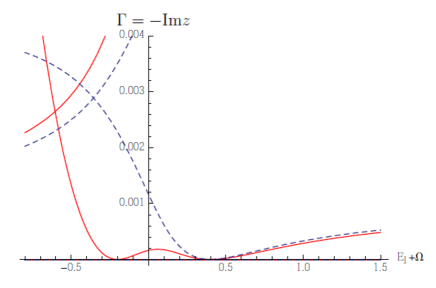
Figure 2: Absolute value of the imaginary part of eigenvalues of the Hamiltonian ($p$-sector) as a function of $\Omega+E_{l}$. The parameters are $T_{1}=0.2,$ $g=0.2,$ $E_{u}=0.1$ and $x_{D}=2.$ The solid line corresponds to $T_{2}=0.2$, while the dashed line corresponds to $T_{2}=0$. The curves on the upper-left corner correspond to another solution of Eq.(24). For $T_{2}=0.2$ (solid line) there is a static BIC at $\Omega+E_{l}=0.4$ which is independent of the strength of the interaction $g$. In addition there is a dynamic BIC at $\Omega+E_{l}=-0.2$ that is due to the interactin with the Fano interference. The $\Omega+E_{l}$ values for which BIC occurs in the plot are consistent with Eqs. (III) and (38), respectively. When $T_{2}=0$ (dashed line) the Fano interference is suppressed, so only the first BIC occurs.

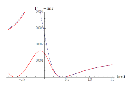
Figure 3: Absolute value of the imaginary part of eigenvalues of the Hamiltonian ($p-$sector) as a function of $\Omega+E_{l}$. The parameters are the same as in figure 2 except for $g=0.4.$ The solid line corresponds to $T_{2}=0.2$, while the dashed line corresponds to $T_{2}=0$. The static BIC that occurs due to the vanishing of the self-energy still occurs at $\Omega+E_{l}=0.4$, while the dynamic BIC is shifted to $\Omega+E_{l}=-0.659$ due to a change of $g$.

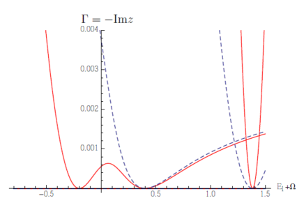
Figure 4: Absolute value of the imaginary part of eigenvalues of the Hamiltonian ($p$-sector) as a function of $\Omega+E_{l}$. The parameters are the same as in figure 2 except for $x_{D}=4.$ The solid line corresponds to $T_{2}=0.2$, while the dashed line corresponds to $T_{2}=0$. There are two BICs at $\Omega+E_{l}=1.38$, and $\Omega+E_{l}=0.4,$ where the self-energy vanishes. There is another BIC at $\Omega+E_{l}=-0.2$, for which the self-energy does not vanish.

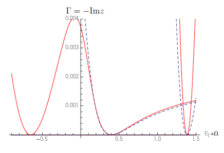
Figure 5: Absolute value of the imaginary part of eigenvalues of the Hamiltonian ($p$-sector) as a function of $\Omega+E_{l}$. The parameters are the same as in figure 4 except for $g=0.4.$ The solid line corresponds to $T_{2}=0.2$, while the dashed line corresponds to $T_{2}=0$. There are two static BICs at $\Omega+E_{l}=1.38$, and $0.4$, while the dynamic BIC is shifted to $\Omega+E_{l}=-0.659$ due to a change of $g$.

In this section we will present numerical results showing the general solution of Eq. (24) as function of $\Omega+E_{l}$ and compare them to the analytic solutions of the BIC we obtained in the previous section. For illustration we will consider the simplest case with $n=0$ where Eq. (III) reduces to a linear equation for $\Omega$. For $n\not=0$, there appear more static BICs than the simplest case with $n=0$. However, in order to demonstrate the essential difference between dynamic BIC and static BIC, it is enough to show the simplest case. The numerical results were obtained through a numerical solution of Eq. (24). In FIGS. 2-5, we plot the imaginary part of the solution, $\Gamma\equiv-\text{Im$z$}$ as a function of $\Omega+E_{l}$ for the $p$-sector. The figures for the $s$-sector are essentially the same as except the locations of BICs are different.

In FIGS. 2-5, we plot the case $E_{l}=0.1$ and $T_{2}=0.2.$ In all these figures the red solid line corresponds to the case $T_{2}=0.2$, and the blue dashed line corresponds to the case $T_{2}=0$. We consider both cases in order to identify the BIC due to Fano interference.

We show in FIG. 2 the case $x_{D}=2$ and $g=0.2$; in FIG. 3 we have the same $x_{D}=2$ but $g=0.4$. As theoretically predicted, we have two BICs, one from Eq.(III) and the other from Eq.(38) with $\Gamma=0$.

The BIC at the positive value of $\Omega+E_{l}$ is the static BIC that exists even in the case $T_{2}=0.$ As one can see, the location of the BIC is at same point in FIG. 2 and FIG. 3, though the value of $g$ is different. The BIC at the negative value of $\Omega+E_{l}$ in FIG. 2 and FIG. 3 is the dynamic BIC that exist only for the case $T_{2}\neq 0.$ The location of this BIC depends on the value of $g$ (compare FIG. 2 and FIG. 3).

We show in FIG. 4 the case $x_{D}=4$ and $g=0.2$; in FIG. 5 we show the case with the same $x_{D}=4$ but $g=0.4$. As predicted, we have different BICs: two are from Eq.(III), and the other from Eq. (38) with $\Gamma=0.$

All the static BICs are located at predicted values of $\Omega+E_{l}$. They exist also in the case $T_{2}=0.$ The location of the static BICs in FIG. 4 appear at the same points in FIG. 5 though the value of $g$ is different. The dynamic BIC appears at the negative values of $\Omega+E_{l}$ in FIG. 4. We have this dynamic BIC only for $T_{2}\neq 0$. The location of the BIC depends on the value $g$ as predicted by Eq. (38).

V Summary

In this paper we have shown tunable bound-states in continuum (BIC) in a 1D quantum wire with two impurities, induced by an intense monochromatic radiation field. We found a new type of BIC in this system that we call “dynamic BIC,” in addition to the other type of BIC that we call “static BIC.” In contrast to the static BIC, the energy of the dynamic BIC depends on the coupling constant $g$ between the discrete state of the electron and the continuous state of the electron. Moreover, we have shown that the dynamic BIC occurs because of the Fano interference among the two transition channels of the electron induced by the radiation field.

Furthermore, we have shown that all BICs obtained in our system exist for any value of $E_{l}$ of the discrete state for a suitable frequency $\Omega$ of the radiation field. This is not the case for the ordinary BIC without the radiation field. In this sense, it is experimentally more feasible to achieve the BIC in our system.

In order to justify experimentally our theoretical results, however, we need the Fano profile of the absorption spectrum of the radiation field Tanaka (5). To construct the Fano profile, we have to construct the eigenstates with the complex eigenvalue of the Hamiltonian for the resonance states (see e.g. Bohm (21)). We hope to present this elsewhere.

References

(1) J. von Neumann and E. Wigner, Phys. Z. ,
465 (1929).