Submodular Optimization with Submodular Cover and Submodular Knapsack Constraints

Abstract

We investigate two new optimization problems — minimizing a submodular function subject to a submodular lower bound constraint (submodular cover) and maximizing a submodular function subject to a submodular upper bound constraint (submodular knapsack). We are motivated by a number of real-world applications in machine learning including sensor placement and data subset selection, which require maximizing a certain submodular function (like coverage or diversity) while simultaneously minimizing another (like cooperative cost). These problems are often posed as minimizing the difference between submodular functions [14, 37] which is in the worst case inapproximable. We show, however, that by phrasing these problems as constrained optimization, which is more natural for many applications, we achieve a number of bounded approximation guarantees. We also show that both these problems are closely related and an approximation algorithm solving one can be used to obtain an approximation guarantee for the other. We provide hardness results for both problems thus showing that our approximation factors are tight up to $\log$-factors. Finally, we empirically demonstrate the performance and good scalability properties of our algorithms.

1 Introduction

A set function $f:2^{V}\to\mathbb{R}$ is said to be submodular [8] if for all subsets $S,T\subseteq V$, it holds that $f(S)+f(T)\geq f(S\cup T)+f(S\cap T)$. Defining $f(j|S)\triangleq f(S\cup j)-f(S)$ as the gain of $j\in V$ in the context of $S\subseteq V$, then $f$ is submodular if and only if $f(j|S)\geq f(j|T)$ for all $S\subseteq T$ and $j\notin T$. The function $f$ is monotone iff $f(j|S)\geq 0,\forall j\notin S,S\subseteq V$. For convenience, we assume the ground set is $V=\{1,2,\cdots,n\}$. While general set function optimization is often intractable, many forms of submodular function optimization can be solved near optimally or even optimally in certain cases, and hence submodularity is also often called the discrete analog of convexity [34]. Submodularity, moreover, is inherent in a large class of real-world applications, particularly in machine learning, therefore making them extremely useful in practice.

In this paper, we study a new class of discrete optimization problems that have the following form:

$$\mbox{Problem 1 (SCSC): }\min\{f(X)\,|\,g(X)\geq c\},\quad\text{and}\quad\mbox{Problem 2 (SCSK): }\max\{g(X)\,|\,f(X)\leq b\},$$

where $f$ and $g$ are monotone non-decreasing submodular functions that also, w.l.o.g., are normalized ($f(\emptyset)=g(\emptyset)=0$), and where $b$ and $c$ refer to budget and cover parameters respectively. The corresponding constraints are called the submodular cover [47] and submodular knapsack [1] respectively and hence we refer to Problem 1 as Submodular Cost Submodular Cover (henceforth SCSC) and Problem 2 as Submodular Cost Submodular Knapsack (henceforth SCSK). Our motivation stems from an interesting class of problems that require minimizing a certain submodular function $f$ while simultaneously maximizing another submodular function $g$. We shall see that these naturally occur in applications like sensor placement, data subset selection, and many other machine learning applications. A standard approach used in literature [14, 37, 22] has been to transform these problems into minimizing the difference between submodular functions (also called DS optimization):

$$\mbox{Problem 0: }\min_{X\subseteq V}\bigl{(}f(X)-g(X)\bigr{)}.$$ (1)

While a number of heuristics are available for solving Problem 0, and while these heuristics often work well in practice [14, 37], in the worst-case it is NP-hard and inapproximable [14], even when $f$ and $g$ are monotone. Although an exact branch and bound algorithm has been provided for this problem [22], its complexity can be exponential in the worst case. On the other hand, in many applications, one of the submodular functions naturally serves as part of a constraint. For example, we might have a budget on a cooperative cost, in which case Problems 1 and 2 become applicable.

1.1 Motivation

The utility of Problems 1 and 2 become apparent when we consider how they occur in real-world applications and how they subsume a number of important optimization problems.

Sensor Placement and Feature Selection: Often, the problem of choosing sensor locations $A$ from a given set of possible locations $V$can be modeled [27, 14] by maximizing the mutual information between the chosen variables $A$ and the unchosen set $V\backslash A$ (i.e.,$f(A)=I(X_{A};X_{V\backslash A})$). Note that, while the symmetric mutual information is not monotone, it can be shown to approximately monotone [27]. Alternatively, we may wish to maximize the mutual information between a set of chosen sensors $X_{A}$ and a quantity of interest $C$ (i.e., $f(A)=I(X_{A};C)$) assuming that the set of features $X_{A}$ are conditionally independent given $C$ [27, 14]. Both these functions are submodular. Since there are costs involved, we want to simultaneously minimize the cost $g(A)$. Often this cost is submodular [27, 14]. For example, there is typically a discount when purchasing sensors in bulk (economies of scale). Moreover, there may be diminished cost for placing a sensor in a particular location given placement in certain other locations (e.g., the additional equipment needed to install a sensor in, say, a precarious environment could be re-used for multiple sensor installations in similar environments). Hence this becomes a form of Problem 2 above. An alternate view of this problem is to find a set of sensors with minimal cooperative cost, under a constraint that the sensors cover a certain fraction of the possible locations, naturally expressed as Problem 1.

Data subset selection: A data subset selection problem in speech and NLP involves finding a limited vocabulary which simultaneously has a large coverage. This is particularly useful, for example in speech recognition and machine translation, where the complexity of the algorithm is determined by the vocabulary size. The motivation for this problem is to find the subset of training examples which will facilitate evaluation of prototype systems [33]. This problem then occurs in the form of Problem 1, where we want to find a small vocabulary subset (which is often submodular [33]), subject to a constraint that the subset acoustically spans the entire data set (which is also often submodular [30, 31]). This can also be phrased as Problem 2, where we ask for maximizing the acoustic coverage and diversity subject to a bounded vocabulary size constraint.

Privacy Preserving Communication: Given a set of random variables $X_{1},\cdots,X_{n}$, denote $\mathfrak{I}$ as an information source, and $\mathfrak{P}$ as private information that should be filtered out. Then one way of formulating the problem of choosing a information containing but privacy preserving set of random variables can be posed as instances of Problems 1 and 2, with $f(A)=H(X_{A}|\mathfrak{I})$ and $g(A)=H(X_{A}|\mathfrak{P})$, where $H(\cdot|\cdot)$ is the conditional entropy. An alternative strategy would be to formulate the problem with $f(A)=H(X_{A})+H(X_{A}|\mathfrak{I})$ and $g(A)=H(X_{A})+H(X_{A}|\mathfrak{P})$.

Machine Translation: Another application in machine translation is to choose a subset of training data that is optimized for given test data set, a problem previously addressed with modular functions [35]. Defining a submodular function with ground set over the union of training and test sample inputs $V=V_{\text{tr}}\cup V_{\text{te}}$, we can set $f:2^{V_{\text{tr}}}\to\mathbb{R}_{+}$ to $f(X)=f(X|V_{\text{te}})$, and take $g(X)=|X|$, and $b\approx 0$ in Problem 2 to address this problem. We call this the Submodular Span problem.

Probabilistic Inference: Many problems in computer vision and graphical model inference involve finding an assignment to a set of random variables. The most-probable explanation (MPE) problem finds the assignment that maximizes the probability. In computer vision and high-tree-width Markov random fields, this has been addressed using graph-cut algorithms  [2], which are applicable when the MRF’s energy function is submodular and limited degree, and more general submodular function minimization in the case of higher degree. Moreover, many useful non-submodular energy functions have also recently been phrased as forms of constrained submodular minimization [20] which still have bounded approximation guarantees. Some of these non-submodular energy functions can be modeled through Problems 1 and 2, where $f$ is still the submodular energy function to be minimized while $g$ represents a submodular constraint. For example, in image co-segmentation [40], $V=V_{1}\cup V_{2}$ can represent the set of pixels in two images, $f$ is the submodular energy function of the two images, while $g$ represents the similarity between the two histograms of the hypothesized foreground regions in the two images, a function shown to be submodular in [40].

Apart from the real-world applications above, both Problems 1 and 2 generalize a number of well-studied discrete optimization problems. For example the Submodular Set Cover problem (henceforth SSC) [47] occurs as a special case of Problem 1, with $f$ being modular and $g$ is submodular. Similarly the Submodular Cost Knapsack problem (henceforth SK) [42] is a special case of problem 2 again when $f$ is modular and $g$ submodular. Both these problems subsume the Set Cover and Max k-Cover problems [6]. When both $f$ and $g$ are modular, Problems 1 and 2 are called knapsack problems [23].Furthermore, Problem 1 also subsumes the cardinality constrained submodular minimization problem [43] and more generally the problem of minimizing a submodular function subject to a knapsack constraints. It also subsumes the problem of minimizing a submodular function subject to a matroid span constraint (by setting $g$ as the rank function of the matroid, and $c$ as the rank of the matroid). This in turn subsumes the minimum submodular spanning tree problem [10], when $f$ is monotone submodular.

1.2 Our Contributions

The following are some of our contributions. We show that Problems 1 and 2 are intimately connected, in that any approximation algorithm for either problem can be used to provide guarantees for the other problem as well. We then provide a framework of combinatorial algorithms based on optimizing, sometimes iteratively, subproblems that are easy to solve. These subproblems are obtained by computing either upper or lower bound approximations of the cost functions or constraining functions. We also show that many combinatorial algorithms like the greedy algorithm for SK [42] and SSC [47] (both of which seemingly use different techniques) also belong to this framework and provide the first constant-factor bi-criterion approximation algorithm for SSC [47] and hence the general set cover problem [6]. We then show how with suitable choices of approximate functions, we can obtain a number of bounded approximation guarantees and show the hardness for Problems 1 and 2, which in fact match some of our approximation guarantees up to $\log$-factors. Our guarantees and hardness results depend on the curvature of the submodular functions [3]. We observe a strong asymmetry in the results that the factors change polynomially based on the curvature of $f$ but only by a constant-factor with the curvature of $g$, hence making the SK and SSC much easier compared to SCSK and SCSC. Finally we empirically evaluate the performance of our algorithms showing that the typical case behavior is much better than these worst case bounds.

2 Background and Main Ideas

We first introduce several key concepts used throughout the paper. Given a submodular function $f$, we define the total curvature, $\kappa_{f}$, and the curvature of $f$ with respect to a set $X$, $\kappa_{f}(X)$, as:

$$\kappa_{f}=1-\min_{j\in V}\frac{f(j|V\backslash j)}{f(j)},\;\;\text{ and }\;\;\kappa_{f}(X)=1-\min\{\min_{j\in X}\frac{f(j|X\backslash j)}{f(j)},\min_{j\notin X}\frac{f(j|X)}{f(j)}\}.$$ (2)

The total curvature $\kappa_{f}$ is then $\kappa_{f}(V)$ [3, 45]. Intuitively, the curvature $0\leq\kappa_{f}\leq 1$ measures the distance of $f$ from modularity and $\kappa_{f}=0$ if and only if $f$ is modular (or additive, i.e., $f(X)=\sum_{j\in X}f(j)$). Totally normalized [4] and saturated functions like matroid rank have a curvature $\kappa_{f}=1$. A number of approximation guarantees in the context of submodular optimization have been refined via the curvature of the submodular function [3, 18, 17]. For example, when maximizing a monotone submodular function under cardinality upper bound constraints, the bound of $1-e^{-1}$ has been refined to $\frac{1-e^{-\kappa_{f}}}{\kappa_{f}}$  [3]. Similar bounds have also been shown in the context of constrained submodular minimization [18, 17, 16]. In this paper, we shall witness the role of curvature also in determining the approximations and the hardness of problems 1 and 2.

1:  for $t=1,2,\cdots,T$ do

2:     Choose surrogate functions $\hat{f_{t}}$ and $\hat{g_{t}}$ for $f$ and $g$ respectively, tight at $X^{t-1}$.

3:     Obtain $X^{t}$ as the optimizer of Problem 1 or 2 with $\hat{f_{t}}$ and $\hat{g_{t}}$ instead of $f$ and $g$.

4:  end for

Algorithm 1 General algorithmic framework to address both Problems 1 and 2

The main idea of this paper is a framework of algorithms based on choosing appropriate surrogate functions for $f$ and $g$ to optimize over. This framework is represented in Algorithm 1. We would like to choose surrogate functions $\hat{f_{t}}$ and $\hat{g_{t}}$ such that using them, Problems 1 and 2 become easier. If the algorithm is just single stage (not iterative), we represent the surrogates as $\hat{f}$ and $\hat{g}$. The surrogate functions we consider in this paper are in the forms of bounds (upper or lower) and approximations. Our algorithms using upper and lower bounds are analogous to the majorization/ minimization algorithms proposed in [18, 16], where we provided a unified framework of fast algorithms for submodular optimization. We show there in that this framework subsumes a large class of known combinatorial algorithms and also providing a generic recipe for different forms of submodular function optimization. We extend these ideas to the more general context of problems 1 and 2, to obtain a fast family of algorithms. The other type of surrogate functions we consider are those obtained from other approximations of the functions. One such classical approximation is the ellipsoidal approximations [11]. While computing this approximation is time consuming, it turns out to provide the tightest theoretical guarantees.

Modular lower bounds: Akin to convex functions, submodular functions have tight modular lower bounds. These bounds are related to the subdifferential $\partial_{f}(Y)$ of the submodular set function $f$ at a set $Y\subseteq V$, which is defined [8] as:

$$\partial_{f}(Y)=\{y\in\mathbb{R}^{n}:f(X)-y(X)\geq f(Y)-y(Y)\;\text{for all }X\subseteq V\}$$ (3)

For a vector $x\in\mathbb{R}^{V}$ and $X\subseteq V$, we write $x(X)=\sum_{j\in X}x(j)$. Denote a subgradient at $Y$ by $h_{Y}\in\partial_{f}(Y)$. The extreme points of $\partial_{f}(Y)$ may be computed via a greedy algorithm: Let $\pi$ be a permutation of $V$ that assigns the elements in $Y$ to the first $|Y|$ positions ($\pi(i)\in Y$ if and only if $i\leq|Y|$). Each such permutation defines a chain with elements $S_{0}^{\pi}=\emptyset$, $S^{\pi}_{i}=\{\pi(1),\pi(2),\dots,\pi(i)\}$ and $S^{\pi}_{|Y|}=Y$. This chain defines an extreme point $h^{\pi}_{Y}$ of $\partial_{f}(Y)$ with entries

$$h^{\pi}_{Y}(\pi(i))=f(S^{\pi}_{i})-f(S^{\pi}_{i-1}).$$ (4)

Defined as above, $h^{\pi}_{Y}$ forms a lower bound of $f$, tight at $Y$ — i.e., $h^{\pi}_{Y}(X)=\sum_{j\in X}h^{\pi}_{Y}(j)\leq f(X),\forall X\subseteq V$ and $h^{\pi}_{Y}(Y)=f(Y)$.

Modular upper bounds: We can also define superdifferentials $\partial^{f}(Y)$ of a submodular function [20, 15] at $Y$:

$$\partial^{f}(Y)=\{y\in\mathbb{R}^{n}:f(X)-y(X)\leq f(Y)-y(Y);\text{for all }X\subseteq V\}$$ (5)

It is possible, moreover, to provide specific supergradients [15, 18, 16] that define the following two modular upper bounds (when referring either one, we use $m^{f}_{X}$):

$$m^{f}_{X,1}(Y)\triangleq f(X)-\!\!\!\!\sum_{j\in X\backslash Y}f(j|X\backslash j)+\!\!\!\!\sum_{j\in Y\backslash X}f(j|\emptyset)\scalebox{1.3}{,}\;\;\;$$

$$m^{f}_{X,2}(Y)\triangleq f(X)-\!\!\!\sum_{j\in X\backslash Y}f(j|V\backslash j)+\!\!\!\!\sum_{j\in Y\backslash X}f(j|X).$$

Then $m^{f}_{X,1}(Y)\geq f(Y)$ and $m^{f}_{X,2}(Y)\geq f(Y),\forall Y\subseteq V$ and $m^{f}_{X,1}(X)=m^{f}_{X,2}(X)=f(X)$.

MM algorithms using upper/lower bounds: Using the modular upper and lower bounds above in Algorithm 1, provide a class of Majorization-Minimization (MM) algorithms, akin to the algorithms proposed in [18, 16] for submodular optimization and in [37, 14] for DS optimization (Problem 0 above). An appropriate choice of the bounds ensures that the algorithm always improves the objective values for Problems 1 and 2. In particular, choosing $\hat{f_{t}}$ as a modular upper bound of $f$ tight at $X^{t}$, or $\hat{g_{t}}$ as a modular lower bound of $g$ tight at $X^{t}$, or both, ensures that the objective value of Problems 1 and 2 always improves at every iteration as long as the corresponding surrogate problem can be solved exactly. Unfortunately, Problems 1 and 2 are NP-hard even if $f$ or $g$ (or both) are modular [6], and therefore the surrogate problems themselves cannot be solved exactly. Fortunately, the surrogate problems are often much easier than the original ones and can admit $\log$ or constant-factor guarantees. In practice, moreover, these factors are almost $1$. In order to guarantee improvement from a theoretical stand-point however, the iterative schemes can be slightly modified using the following trick. Notice that the only case when the true valuation of $X^{t}$ is better than $X^{t+1}$ is when the surrogate valuation of $X^{t}$ is better than $X^{t+1}$ (since $X^{t+1}$ is only near-optimal and not optimal). In such case, we terminate the algorithm at $X^{t}$. What is also fortunate and perhaps surprising, as we show in this paper below, is that unlike the case of DS optimization (where the problem is inapproximable in general [14]), the constrained forms of optimization (Problems 1 and 2) do have approximation guarantees.

Ellipsoidal Approximation: We also consider ellipsoidal approximations (EA) of $f$. The main result of Goemans et.  al [11] is to provide an algorithm based on approximating the submodular polyhedron by an ellipsoid. They show that for any polymatroid function $f$, one can compute an approximation of the form $\sqrt{w^{f}(X)}$ for a certain modular weight vector $w^{f}\in\mathbb{R}^{V}$, such that $\sqrt{w^{f}(X)}\leq f(X)\leq O(\sqrt{n}\log{n})\sqrt{w^{f}(X)},\forall X\subseteq V$. A simple trick then provides a curvature-dependent approximation [17] — we define the $\kappa_{f}$-curve-normalized version of $f$ as follows:

$$f^{\kappa}(X)\triangleq\frac{f(X)-{(1-\kappa_{f})}\sum_{j\in X}f(j)}{\kappa_{f}}.$$ (6)

The function $f^{\kappa}$ essentially contains the zero curvature component of the submodular function $f$ and the modular upper bound $\sum_{j\in X}f(j)$ contains all the linearity. The main idea is to then approximate only the polymatroidal part and retain the linear component. This simple trick improves many of the approximation bounds. We then have the following lemma.

Lemma 2.1.

[17] Given a polymatroid function $f$ with a curvature $\kappa_{f}<1$, the submodular function $f^{\text{ea}}(X)=\kappa_{f}\sqrt{w^{f^{\kappa}}(X)}+(1-\kappa_{f})\sum_{j\in X}f(j)$ satisfies:

$$f^{\text{ea}}(X)\leq f(X)\leq O\left(\frac{\sqrt{n}\log{n}}{1+(\sqrt{n}\log{n}-1)(1-\kappa_{f})}\right)f^{\text{ea}}(X),\forall X\subseteq V$$ (7)

$f^{\text{ea}}$ is multiplicatively bounded by $f$ by a factor depending on $\sqrt{n}$ and the curvature. The dependence on the curvature is evident from the fact that when $\kappa_{f}=0$, we get a bound of $O(1)$, which is not surprising since a modular $f$ is exactly represented as $f(X)=\sum_{j\in X}f(j)$. We shall use the result above in providing approximation bounds for Problems 1 and 2. In particular, the surrogate functions $\hat{f}$ or $\hat{g}$ in Algorithm 1 can be the ellipsoidal approximations above, and the multiplicative bounds transform into approximation guarantees for these problems.

3 Relation between SCSC and SCSK

In this section, we show a precise relationship between Problems 1 and 2. From the formulation of Problems 1 and 2, it is clear that these problems are duals of each other. Indeed, in this section we show that the problems are polynomially transformable into each other.

1:  Input: An SCSK instance with budget $b$, an $[\sigma,\rho]$ approx. algo. for SCSC, & $\epsilon>0$.

2:  Output: $[(1-\epsilon)\rho,\sigma]$ approx. for SCSK.

3:  $c\leftarrow g(V),\hat{X_{c}}\leftarrow V$.

4:  while $f(\hat{X_{c}})>\sigma b$ do

5:     $c\leftarrow(1-\epsilon)c$

6:     $\hat{X_{c}}\leftarrow[\sigma,\rho]$ approx. for SCSC using $c$.

7:  end while

8:  Return $\hat{X}_{c}$

Algorithm 2 Approx. algorithm for SCSK using an approximation algorithm for SCSC using Linear search.

1:  Input: An SCSC instance with cover $c$, an $[\rho,\sigma]$ approx. algo. for SCSK, & $\epsilon>0$.

2:  Output: $[(1+\epsilon)\sigma,\rho]$ approx. for SCSC.

3:  $b\leftarrow\operatorname*{argmin}_{j}f(j),\hat{X_{b}}\leftarrow\emptyset$.

4:  while $g(\hat{X_{b}})<\rho c$ do

5:     $b\leftarrow(1+\epsilon)b$

6:     $\hat{X_{b}}\leftarrow[\rho,\sigma]$ approx. for SCSK using $b$.

7:  end while

8:  Return $\hat{X}_{b}$.

Algorithm 3 Approx. algorithm for SCSC using an approximation algorithm for SCSK using Linear search.

Figure 1: Bicriterion transformation algorithms for SCSC and SCSK using Linear search.

We first introduce the notion of bicriteria algorithms. An algorithm is a $[\sigma,\rho]$ bi-criterion algorithm for Problem 1 if it is guaranteed to obtain a set $X$ such that $f(X)\leq\sigma f(X^{*})$ (approximate optimality) and $g(X)\geq c^{\prime}=\rho c$ (approximate feasibility), where $X^{*}$ is an optimizer of Problem 1. Similarly, an algorithm is a $[\rho,\sigma]$ bi-criterion algorithm for Problem 2 if it is guaranteed to obtain a set $X$ such that $g(X)\geq\rho g(X^{*})$ and $f(X)\leq b^{\prime}=\sigma b$, where $X^{*}$ is the optimizer of Problem 2. In a bi-criterion algorithm for Problems 1 and 2, typically $\sigma\geq 1$ and $\rho\leq 1$. We call these type of approximation algorithms, bi-criterion approximation algorithms of type 1.

We can also view the bi-criterion approximations from another angle. We can say that for Problem 1, $\hat{X}$ is a feasible solution (i.e., it satisfies the constraint), and is a $[\sigma,\rho]$ bi-criterion approximation, if $f(\hat{X})\leq\sigma f(\hat{X}^{*})$, where $\hat{X}^{*}$ is the optimal solution to the problem $\min\{f(X)|g(X)\geq c/\rho\}$. Similarly for Problem 2, we can say that $\hat{X}$ is a feasible solution (i.e., it satisfies the constraint), and is a $[\rho,\sigma]$ bi-criterion approximation, if $g(\hat{X})\geq\rho g(\hat{X}^{*})$, where $\hat{X}^{*}$ is the optimal solution to the problem $\max\{g(X)|f(X)\leq b\sigma\}$. We call these the bi-criterion approximation algorithms of type 2.

It is easy to see that these algorithms can easily be transformed into each other. For example, for problem 1, a bi-criterion algorithm of type-I can obtain a guarantee of type-II if we run it till a covering constraint of $c^{\prime}/\rho$ (where $c^{\prime}$ in this case, is the approximate covering constraint which the type-I algorithm needs to satisfy – note that it need not be the actual covering constraint of the problem). Similarly an algorithm of type-II can obtain a guarantee of type-I if run till a covering constraint of $\rho c$ (in this case, $c$ is the actual ’covering’ constraint, since a type-II approximate algorithm provides a feasible set). We can similarly transform these guarantees for problem 2. In particular, a bi-criterion algorithm of type-I can be used to obtain a guarantee of type-II if we run it till a budget of $b^{\prime}\sigma$ (again, here $b^{\prime}$ is the approximate budget of the type-I algorithm). Similarly an algorithm of type-II can obtain a guarantee of type-I if run till a covering constraint of $b/\sigma$ (in this case, $b$ is the budget of the original problem).

Though both type-I and type-II guarantees are easily transformable into each other, through the rest of this paper whenever we refer to bi-criterion approximations, we shall consider only the type-I approximations. A non-bicriterion algorithm for Problem 1 is when $\rho=1$ and a non-bicriterion algorithm for Problem 2 is when $\sigma=1$. Algorithms 2 and 3 provide the schematics for using an approximation algorithm for one of the problems for solving the other.

The main idea of Algorithm 2 is to start with the ground set $V$ and reduce the value of $c$ (which governs SCSC), until the valuation of $f$ just falls below $\sigma b$. At that point, we are guaranteed to get a $((1-\epsilon)\rho,\sigma)$ solution for SCSK. Similarly in Algorithm 3, we increase the value of $b$ starting at the empty set, until the valuation at $g$ falls above $\rho c$. At this point we are guaranteed a $((1+\epsilon)\sigma,\rho)$ solution for SCSC. In order to avoid degeneracies, we assume that $f(V)\geq b\geq\min_{j}f(j)$ and $g(V)\geq c\geq\min_{j}g(j)$, else the solution to the problem is trivial.

Theorem 3.1.

Algorithm 2 is guaranteed to find a set $\hat{X_{c}}$ which is a $[(1-\epsilon)\rho,\sigma]$ approximation of SCSK in at most $\log_{1/(1-\epsilon)}[g(V)/\min_{j}g(j)]$ calls to the $[\sigma,\rho]$ approximate algorithm for SCSC. Similarly, Algorithm 3 is guaranteed to find a set $\hat{X_{b}}$ which is a $[(1+\epsilon)\sigma,\rho]$ approximation of SCSC in $\log_{1+\epsilon}[f(V)/\min_{j}f(j)]$ calls to a $[\rho,\sigma]$ approximate algorithm for SCSK.

Proof.

We start by proving the first part, for Algorithm 2. Notice that Algorithm 2 converges when $f(\hat{X_{c}})$ just falls below $\sigma b$. Hence $f(\hat{X_{c}})\leq\sigma b$ (is approximately feasible) and at the previous step $c^{\prime}=c/(1-\epsilon)$, we have that $f(\hat{X_{c^{\prime}}})>\sigma b$. Denoting $X^{*}_{c^{\prime}}$ as the optimal solution for SCSC at $c^{\prime}$, we have that $f(X^{*}_{c^{\prime}})>b$ (a fact which follows from the observation that $\hat{X_{c}}$ is a $[\sigma,\rho]$ approximation of SCSC at $c$). Hence if $X^{*}$ is the optimal solution of SCSK, it follows that $g(X^{*})<c^{\prime}$. The reason for this is that, suppose, $g(X^{*})\geq c^{\prime}$. Then it follows that $X^{*}$ is a feasible solution for SCSC at $c^{\prime}$ and hence $f(X^{*})\geq f(X^{*}_{c^{\prime}})>b$. This contradicts the fact that $X^{*}$ is an optimal solution for SCSK (since it is then not even feasible).

Next, notice that $\hat{X_{c}}$ satisfies that $g(\hat{X_{c}})\geq\rho c$, using the fact that $\hat{X_{c}}$ is obtained from a $(\sigma,\rho)$ bi-criterion algorithm for SCSC. Hence,

$$g(\hat{X_{c}})\geq\rho c=\rho(1-\epsilon)c^{\prime}>\rho(1-\epsilon)g(X^{*})$$ (8)

Hence the Algorithm 2 is a $((1-\epsilon)\rho,\sigma)$ approximation for SCSK. In order to show the converge rate, notice that $c\geq\min_{j}g(j)>0$. Since $\sigma\geq 1$ and $b\geq\min_{j}f(j)$, we can guarantee that this algorithm will stop before $c$ reaches $\min_{j}g(j)$. The reason is that, when $c=\min_{j}g(j)$, the minimum value of $f(X)$ such that $g(X)\geq c$ is $\min_{j}f(j)$, which is smaller than $b$. Moreover, since $\sigma>1$, it implies that the algorithm would have terminated before this point.

The proof for the second part of the statement, for Algorithm 3, is omitted since it is shown using a symmetric argument. ∎

1:  Input: An SCSK instance with budget $b$, an $[\sigma,\rho]$ approx. algo. for SCSC, & $\epsilon>0$.

2:  Output: $[(1-\epsilon)\rho,\sigma]$ approx. for SCSK.

3:  $c_{\min}\leftarrow\min_{j}g(j),c_{\max}\leftarrow g(V)$

4:  while $c_{\max}-c_{\min}\geq\epsilon c_{\max}$  do

5:     $c\leftarrow[c_{\max}+c_{\min}]/2$

6:     $\hat{X_{c}}\leftarrow[\sigma,\rho]$ approx. for SCSC using $c$.

7:     if $f(\hat{X_{c}})>\sigma b$ then

8:        $c_{\max}\leftarrow c$

9:     else

10:        $c_{\min}\leftarrow c$

11:     end if

12:  end while

13:  Return $\hat{X}_{c_{\min}}$

Algorithm 4 Approx. algorithm for SCSK using an approximation algorithm for SCSC using Binary search.

1:  Input: An SCSC instance with cover $c$, an $[\rho,\sigma]$ approx. algo. for SCSK, & $\epsilon>0$.

2:  Output: $[(1+\epsilon)\sigma,\rho]$ approx. for SCSC.

3:  $b_{\min}\leftarrow\operatorname*{argmin}_{j}f(j),b_{\max}\leftarrow f(V)$.

4:  while $b_{\max}-b_{\min}\geq\epsilon b_{\min}$  do

5:     $b\leftarrow[b_{\max}+b_{\min}]/2$

6:     $\hat{X_{b}}\leftarrow[\rho,\sigma]$ approx. for SCSK using $b$

7:     if $g(\hat{X_{b}})<\rho c$ then

8:        $b_{\min}\leftarrow b$

9:     else

10:        $b_{\max}\leftarrow b$

11:     end if

12:  end while

13:  Return $\hat{X}_{b_{\max}}$

Algorithm 5 Approx. algorithm for SCSC using an approximation algorithm for SCSK using Binary search.

Figure 2: Bicriterion transformation algorithms for SCSC and SCSK using Binary search.

Theorem 3.1 implies that the complexity of Problems 1 and 2 are identical, and a solution to one of them provides a solution to the other. Furthermore, as expected, the hardness of Problems 1 and 2 are also almost identical. When $f$ and $g$ are polymatroid functions, moreover, we can provide bounded approximation guarantees for both problems, as shown in the next section.

Alternatively we can also do a binary search instead of a linear search to transform Problems 1 and 2. This essentially turns the factor of $O(1/\epsilon)$ into $O(\log 1/\epsilon)$. Algorithms 4 and 5 show the transformation algorithms using binary search. While the binary search also ensures the same performance guarantees, it does so more efficiently.

Theorem 3.2.

Algorithm 4 is guaranteed to find a set $\hat{X_{c}}$ which is a $[(1-\epsilon)\rho,\sigma]$ approximation of SCSK in at most $\log_{2}\frac{[g(V)/\min_{j}g(j)]}{\epsilon}$ calls to the $[\sigma,\rho]$ approximate algorithm for SCSC. Similarly, Algorithm 5 is guaranteed to find a set $\hat{X_{b}}$ which is a $[(1+\epsilon)\sigma,\rho]$ approximation of SCSC in $\log_{2}\frac{[f(V)/\min_{j}f(j)]}{\epsilon}$ calls to a $[\rho,\sigma]$ approximate algorithm for SCSK. When $f$ and $g$ are integral, moreover, Algorithm 4 obtains a $[\rho,\sigma]$ bi-criterion approximate solution for SCSK in $\log_{2}g(V)$ iterations, and similarly Algorithm 5 obtains a $[\sigma,\rho]$ bi-criterion approximate solution for SCSC in $\log_{2}g(V)$ iterations.

Proof.

To show this theorem, we use the result from Theorem 3.1. Let $c=c_{\min}$ and $c^{\prime}=c_{\max}$. An important observation is that throughout the algorithm, the values of $c_{\min}$ satisfy $f(\hat{X}_{c_{\min}})\leq\sigma b$ and $f(\hat{X}_{c_{\max}})>\sigma b$. Hence, $f(\hat{X_{c}})\leq\sigma b$ and $f(\hat{X_{c^{\prime}}})>\sigma b$. Moreover, notice that $c^{\prime}/c=c_{\max}/c_{\min}=1/(1-\epsilon)$. Hence using the proof of Theorem 3.1 the approximation guarantee follows.

In order to show the complexity, notice that $c_{\max}-c_{\min}$ is decreasing throughout the algorithm. At the beginning, $c_{\max}-c_{\min}\leq g(V)$ and at convergence, $c_{\max}-c_{\min}\geq\epsilon c_{\max}/2\geq\epsilon\min_{j}g(j)/2$. The bound at convergence holds since, let $c^{\prime}_{max}$ and $c^{\prime}_{min}$ be the values at the previous step. It holds that $c^{\prime}_{\max}-c^{\prime}_{\min}\geq\epsilon c^{\prime}_{\max}$. Moreover, $c_{max}-c_{min}=(c^{\prime}_{\max}-c^{\prime}_{\min})/2\geq\epsilon c^{\prime}_{\max}/2\geq\epsilon c_{\max}$. Hence the number of iterations is bounded by $\log_{2}\frac{[2g(V)/\min_{j}g(j)]}{\epsilon}$. Moreover, when $f$ and $g$ are integral, the analysis is much simpler. In particular, notice that once $c_{max}-c_{min}=1$, the algorithm will stop at the next iteration (this is because at this point, $c=(c_{max}+c_{min})/2$ is equivalent to $c=c_{max}$). Hence, the number of iterations is bounded by $\log_{2}g(V)$, and we can exactly obtain a $[\rho,\sigma]$ bi-criterion approximation algorithm.

The proof for the second part of the statement, for Algorithm 3, similarly follows using a symmetric argument.

∎

When $f$ and $g$ are integral, this removes the $\epsilon$ dependence on the factors and could potentially be much faster in practice. We also remark that a specific instance of such a transformation has been used [26], for a specific class of functions $f$ and $g$. We shall show in section 4.3 that their algorithm is in fact a special case of Algorithm 4 through a specific construction to convert the non-submodular problem into an instance of a submodular one.

Algorithm 2 and Algorithm 3 indeed provide an interesting theoretical result connecting the complexity of Problems 1 and 2. In the next section however, we provide distinct algorithms for each problem when $f$ and $g$ are polymatroid functions — this turns out to be faster than having to resort to the iterative reductions above.

4 Approximation Algorithms

We consider several algorithms for Problems 1 and 2, which can all be characterized by the framework of Algorithm 1, using the surrogate functions of the form of upper/lower bounds or approximations.

4.1 Approximation Algorithms for SCSC

We first describe our approximation algorithms designed specifically for SCSC, leaving to §4.2 the presentation of our algorithms slated for SCSK. We first investigate a special case, the submodular set cover (SSC), and then provide two algorithms, one of them (ISSC) is very practical with a weaker theoretical guarantee, and another one (EASSC) which is slow but has the tightest guarantee.

Submodular Set Cover (SSC): We start by considering a classical special case of SCSC (Problem 1) where $f$ is already a modular function and $g$ is a submodular function. This problem occurs naturally in a number of problems related to active/online learning [12] and summarization [31, 32]. This problem was first investigated by Wolsey [47], wherein he showed that a simple greedy algorithm achieves bounded (in fact, log-factor) approximation guarantees. We show that this greedy algorithm can naturally be viewed in the framework of our Algorithm 1 by choosing appropriate surrogate functions $\hat{f_{t}}$ and $\hat{g_{t}}$. The idea is to use the modular function $f$ as its own surrogate $\hat{f_{t}}$ and choose the function $\hat{g_{t}}$ as a modular lower bound of $g$. Akin to the framework of algorithms in [18], the crucial factor is the choice of the lower bound (or subgradient). Define the greedy subgradient (equivalently the greedy permutation) as:

$$\pi(i)\in\operatorname*{argmin}\left\{\frac{f(j)}{g(j|S^{\pi}_{i-1})}\ \bigg{|}\ j\notin S^{\pi}_{i-1},g(S^{\pi}_{i-1}\cup j)<c\right\}.$$ (9)

Once we reach an $i$ where the constraint $g(S^{\pi}_{i-1}\cup j)<c$ can no longer be satisfied by any $j\notin S^{\pi}_{i-1}$, we choose the remaining elements for $\pi$ arbitrarily. Let the corresponding subgradient be referred to as $h^{\pi}$. Let $N$ be the minimum $i$ such that $g(S^{\pi}_{i})\geq c$ and $\theta_{i}=\min_{j\notin S^{\pi}_{i-1}}\frac{f(j)}{g(j|S^{\pi}_{i-1})}$. Then we have the following lemma, which is an extension of [47]:

Lemma 4.1.

Choosing the surrogate function $\hat{f}$ as $f$ and $\hat{g}$ as $h^{\pi}$ (with $\pi$ defined in Eqn. (9)) in Algorithm 1, at the end of the first iteration, we are guaranteed to obtain a set $X^{g}$ such that

$$\frac{f(X^{g})}{f(X^{*})}\leq 1+\log_{e}\min\{\lambda_{1},\lambda_{2},\lambda_{3}\}$$ (10)

where $\lambda_{1}=\max\{\frac{1}{1-\kappa_{g}(S^{\pi}_{i})}|\ i:c(S^{\pi}_{i})<1\}$, $\lambda_{2}=\frac{\theta_{N}}{\theta_{1}}$ and $\lambda_{3}=\frac{g(V)-g(\emptyset)}{g(V)-g(S^{\pi}_{N-1})}$. Furthermore if $g$ is integral, $\frac{f(X^{g})}{f(X^{*})}\leq H(\max_{j}g(j))$, where $H(d)=\sum_{i=1}^{d}\frac{1}{i}$ for a positive integer $d$.

Proof.

The permutation $\pi$ is chosen based on a greedy ordering associated with the submodular set cover problem, and therefore $h^{\pi}(S^{\pi}_{N})=g(S^{\pi}_{N})\geq c$ (where the inequality follows from the definition of $N$), and thus $S^{\pi}_{N}$ is a feasible solution in the surrogate problem (where $g$ is replaced by $h^{\pi}$). The resulting knapsack problem can be addressed using the greedy algorithm [23], but this exactly corresponds to the greedy algorithm of submodular set cover [47] and hence the guarantee follows from Theorem 1 in [47]. ∎

The surrogate problem in this instance is a simple knapsack problem that can be solved nearly optimally using dynamic programming [44]. As stated in the proof, the greedy algorithm for the submodular set cover problem [47] is in fact equivalent to using the greedy algorithm for the knapsack problem [23], which is in fact suboptimal. When $g$ is integral, the guarantee of the greedy algorithm is $H_{g}\triangleq H(\max_{j}g(j))$, where $H(d)=\sum_{i=1}^{d}\frac{1}{i}$ [47] (henceforth we will use $H_{g}$ for this quantity). This factor is tight up to lower-order terms [6]. Furthermore, since this algorithm directly solves SSC, we call it the primal greedy. We could also solve SSC by looking at its dual, which is SK [42]. Although SSC does not admit any constant-factor approximation algorithms [6], we can obtain a constant-factor bi-criterion guarantee:

Lemma 4.2.

Using the greedy algorithm for SK [42] as the approximation oracle in Algorithm 3 provides a $[1+\epsilon,1-e^{-1}]$ bi-criterion approximation algorithm for SSC, for any $\epsilon>0$.

Proof.

We call this the dual greedy. This result follows immediately from the guarantee of the submodular cost knapsack problem [42] and Theorem 3.1. ∎

We remark that we can also use a simpler version of the greedy iteration at every iteration [31, 24] and we obtain a guarantee of $(1+\epsilon,1/2(1-e^{-1}))$. In practice, however, both these factors are almost $1$ and hence the simple variant of the greedy algorithm suffices.

An interesting connection between the greedy algorithm and the induced orderings, allows us to further simplify this dual algorithm. A nice property of the greedy algorithm for the submodular knapsack problem is that it can be completely parameterized by the chain of sets (this holds for the greedy algorithm of [31, 24] for knapsack constraints and the basic greedy algorithm of [38] under cardinality constraints). In particular, having computed the greedy chain of sets, and given a value of $b$ or the budget, we can easily find the corresponding set in $O(\log n)$ time using binary search. Moreover, this also implies that we can do the transformation algorithms by just iterating through the chain of sets once. In particular, the linear search over the different values of $\epsilon$ is equivalent to the linear search over the different chain of sets. Moreover, we could also do the much faster binary search. Hence the complexity of the dual greedy algorithm is almost identical to the primal greedy one for the submodular set cover problem.

It is also important to put the bicriterion result into perspective. Notice that the bicriterion guarantee suggests that we find only an approximate feasible solution. In particular, the dual greedy algorithm provides a type-I bi-criterion approximation, – that the solution obtained by running the algorithm with a cover constraint of $(1-1/e)c$ is competitive to the optimal solution with a cover constraint of $c$. However, we can also obtain a type-II bi-criterion approximation by running the dual greedy algorithm until it satisfies the cover constraint of $c$. In this case, we would obtain a feasible solution. The guarantee, however, would say that the resulting solution would be competitive to the optimal solution obtained with a cover constraint of $c/(1-e^{-1})$. Furthermore, these factors are in practice close to $1$, and the primal and dual greedy algorithms would both perform very well empirically.

Iterated Submodular Set Cover (ISSC): We next investigate an algorithm for the general SCSC problem when both $f$ and $g$ are submodular. The idea here is to iteratively solve the submodular set cover problem which can be done by replacing $f$ by a modular upper bound at every iteration. In particular, this can be seen as a variant of Algorithm 1, where we start with $X^{0}=\emptyset$ and choose $\hat{f_{t}}(X)=m^{f}_{X^{t},2}(X)$ at every iteration (alternatively, we can choose $\hat{f_{t}}(X)=m^{f}_{X^{t},1}(X)$). At the first iteration with $X^{0}=\emptyset$, either variant then corresponds to the set cover problem with the simple modular upper bound $f(X)\leq m^{f}_{\emptyset}(X)=\sum_{j\in X}f(j)$ where $m^{f}_{X^{t}}$ refers to either variant. The surrogate problem at each iteration becomes:

minimize $$m^{f}_{X^{t}}(X)$$

subject to $$g(X)\geq c.$$

Hence, each iteration is an instance of SSC and can be solved nearly optimally using the greedy algorithm. We can continue this algorithm for $T$ iterations or until convergence. An analysis very similar to the ones in [14, 18] will reveal polynomial time convergence. Since each iteration is only the greedy algorithm, this approach is also highly practical and scalable. Since there are two approaches to solve the set cover problem (the primal approach of Lemma 4.1 and the dual greedy approach of Lemma 4.2), we have two forms of ISSC, the primal ISSC and the dual ISSC. The following shows the resulting theoretical guarantees:

Theorem 4.3.

The primal ISSC algorithm obtains an approximation factor of $\frac{K_{g}H_{g}}{1+(K_{g}-1)(1-\kappa_{f})}\leq\frac{n}{1+(n-1)(1-\kappa_{f})}H_{g}$ where $K_{g}=1+\max\{|X|:g(X)<c\}$ and $H_{g}$ is the approximation factor of the submodular set cover using $g$. Similarly the dual ISSC obtains a bi-criterion guarantee of $\left[\frac{(1+\epsilon)K_{g}}{1+(K_{g}-1)(1-\kappa_{f})},1-e^{-1}\right]$.

Proof.

The first part of the result follows directly from Theorem 5.4 in [18]. In particular, the result from [18] ensures a guarantee of

$$\frac{\beta|X^{*}|}{1+(|X^{*}|-1)(1-\kappa_{f})}$$ (11)

for the problem of $\min\{f(X)|X\in\mathcal{C}\}$ where $\beta$ is the approximation guarantee of solving a modular function over $\mathcal{C}$ where $\mathcal{C}$ is the feasible set. In this case, $\beta=H_{g}$ and $|X^{*}|\leq K_{g}$.

When using the dual greedy approach at every iteration, we can use a similar form of the result in the bi-criterion sense. Consider only the first iteration of this algorithm (due to the monotonicity of the algorithm, we will only improve the objective value). We are then guaranteed to obtain a set $\hat{X}$ such that (denote $X^{1}$ as the solution after the first iteration)

$$f(\hat{X})\leq f(X^{1})\leq m^{f}_{\emptyset}(X^{1})\leq(1+\epsilon)m^{f}_{\emptyset}(X^{*})\leq\frac{K_{g}(1+\epsilon)}{1+(K_{g}-1)(1-\kappa_{f})}f(X^{*})$$ (12)

The inequalities above follow from the fact that the modular upper bound $m^{f}_{\emptyset}(X)$ satisfies [17],

$$m^{f}_{\emptyset}(X)\leq f(X)\leq\frac{|X|}{1+(|X|-1)(1-\kappa_{f})}f(X)$$ (13)

and the fact that $X^{1}$ which is the solution obtained through the dual set cover with a cover constraint $(1-e^{-1})c$ satisfies $m^{f}_{\emptyset}(X^{1})\leq(1+\epsilon)m^{f}_{\emptyset}(X^{*})$. In the above, $X^{*}$ is the optimal solution to the problem $\min\{f(X)|g(X)\geq c\}$. We could also run the dual set cover algorithm to obtain a feasible solution (i.e., a type-II guarantee). In this case, the guarantee would compete with the optimal solution satisfying a cover constraint of $c/(1-e^{-1})$. ∎

From the above, it is clear that $K_{g}\leq n$. Notice also that $H_{g}$ is essentially a log-factor. We also see an interesting effect of the curvature $\kappa_{f}$ of $f$. When $f$ is modular ($\kappa_{f}=0$), we recover the approximation guarantee of the submodular set cover problem. Similarly, when $f$ has restricted curvature, the guarantees can be much better. For example, using square-root over modular function $f(X)=\sum_{i=1}^{k}\sqrt{w_{i}(X)}$, which is common model used in applications [14, 29, 19], the worst case guarantee is $H_{g}\sqrt{K_{g}}$. This follows directly from the results in [17]. Moreover, the approximation guarantee already holds after the first iteration, so additional iterations can only further improve the objective.

We remark here that a special case of ISSC, using only the first iteration (i.e., the simple modular upper bound of $f$) was considered in [46, 5]. Our algorithm not only possibly improves upon theirs, but our approximation guarantee is also more explicit than theirs. In particular, they show a guarantee of $\nu_{f}H_{g}$, where $\nu_{f}=\min\{\frac{\sum_{i\in X}f(i)}{f(X)}|g(X)=g(V)\}$. Since this factor $\nu_{f}$ itself involves an optimization problem, it is not clear how to efficiently compute this factor. Moreover given a submodular function $f$, it is also not evident how good this factor is. While our guarantee is an upper bound of $\nu_{f}H_{g}$, it is much more explicit in it’s dependence on the parameters of the problem. It can also be computed efficiently and has an intuitive significance related to the curvature of the function. Furthermore, our bound is also tight since with, for example, $f(X)=\min\{|X|,1\}$, our exactly matches the bound of [46, 5]. Lastly our algorithm also potentially improves upon theirs thanks to it’s iterative nature.

For another variant of this algorithm, we can replace $g$ with its greedy modular lower bound at every iteration. Then, rather than solving every iteration through the greedy algorithm, we can solve every iteration as a knapsack problem (minimizing a modular function over a modular lower bound constraint) [23], using say, a dynamic programming based approach. This could potentially improve over the greedy variant, but at a potentially higher computational cost.

Ellipsoidal Approximation based Submodular Set Cover (EASSC): In this setting, we use the ellipsoidal approximation discussed in §2. We can compute the $\kappa_{f}$-curve-normalized version of $f$ ($f^{\kappa}$, see §2), and then compute its ellipsoidal approximation $\sqrt{w^{f^{\kappa}}}$. We then define the function $\hat{f}(X)=f^{\text{ea}}(X)=\kappa_{f}\sqrt{w^{f^{\kappa}}(X)}+(1-\kappa_{f})\sum_{j\in X}f(j)$ and use this as the surrogate function $\hat{f}$ for $f$. We choose $\hat{g}$ as $g$ itself. The surrogate problem becomes:

$$\min\left\{\kappa_{f}\sqrt{w^{f^{\kappa}}(X)}+(1-\kappa_{f})\sum_{j\in X}f(j)\ \bigg{|}\ g(X)\geq c\right\}.$$ (14)

While function $\hat{f}(X)=f^{\text{ea}}(X)$ is not modular, it is a weighted sum of a concave over modular function and a modular function. Fortunately, we can use the result from [39], where they show that any function of the form of $\sqrt{w_{1}(X)}+w_{2}(X)$ can be optimized over any polytope $\mathcal{P}$ with an approximation factor of $\beta(1+\epsilon)$ for any $\epsilon>0$, where $\beta$ is the approximation factor of optimizing a modular function over $\mathcal{P}$. The complexity of this algorithm is polynomial in $n$ and $\frac{1}{\epsilon}$. The main idea of their paper is to reduce the problem of minimizing $\sqrt{w_{1}(X)}+w_{2}(X)$, into $\log n$ problems of minimizing a modular function over the polytope. We use their algorithm to minimize $f^{\text{ea}}(X)$ over the submodular set cover constraint and hence we call this algorithm EASSC. Again we have the two variants, primal EASSC and dual EASSC, which essentially use at every iteration the primal and dual forms of set cover.

Theorem 4.4.

The primal EASSC obtains a guarantee of $O(\frac{\sqrt{n}\log nH_{g}}{1+(\sqrt{n}\log n-1)(1-\kappa_{f})})$, where $H_{g}$ is the approximation guarantee of the set cover problem. Moreover, the dual EASSC obtains a bi-criterion approximation of $\left[O(\frac{\sqrt{n}\log n}{1+(\sqrt{n}\log n-1)(1-\kappa_{f})}),1-e^{-1}\right]$.

Proof.

The idea of the proof is to use the result from [39] where they show that any function of the form $\lambda_{1}\sqrt{m_{1}(X)}+\lambda_{2}m_{2}(X)$ where $\lambda_{1}\geq 0,\lambda_{2}\geq 0$ and $m_{1}$ and $m_{2}$ are positive modular functions has a FPTAS, provided a modular function can easily be optimized over $\mathcal{C}$. Note that our function is exactly of that form. Hence, $\hat{f}(X)$ can be approximately optimized over $\mathcal{C}$. It now remains to show that this translates into the approximation guarantee. From Lemma 2.1, we know that there exists a $\hat{f}$ such that $\hat{f}(X)\leq f(X)\leq\beta(n)\hat{f}(X),\forall X$ where

$$\beta(n)=O\left(\frac{\sqrt{n}\log n}{(\sqrt{n}\log n-1)(1-\kappa_{f})+1)}\right).$$ (15)

Then, if $\hat{X}$ is the $1+\epsilon$ approximately optimal solution for minimizing $\hat{f}$ over $\{X:g(X)\geq c\}$, we have that:

$$f(\hat{X})\leq\beta(n)\hat{f}(\hat{X})\leq H_{g}\beta(n)(1+\epsilon)\hat{f}(X^{*})\leq H_{g}\beta(n)(1+\epsilon)f(X^{*}),$$ (16)

where $X^{*}$ is the optimal solution. We can set $\epsilon$ to any constant, say $1$, and we get the result.

The dual guarantee again follows in a very similar manner thanks to the guarantee for the dual SSC. ∎

If the function $f$ has $\kappa_{f}=1$, we can use a much simpler algorithm. In particular, since the ellipsoidal approximation is of the form of $f^{\text{ea}}(X)=\sqrt{w^{f}(X)}$, we can minimize $(f^{\text{ea}}(X))^{2}=w^{f}(X)$ at every iteration, giving a surrogate problem of the form

$$\min\{w^{f}(X)|g(X)\geq c\}.$$ (17)

This is directly an instance of SSC, and in contrast to EASSC, we just need to solve SSC once. We call this algorithm EASSCc. This guarantee is tight up to $\log$ factors when $\kappa_{f}=1$.

Corollary 4.5.

The primal EASSCc obtains an approximation guarantee of $O(\sqrt{n}\log n\sqrt{H_{g}})$. Similarly, the dual EASSCc obtains a bicriterion guarantee of $[O(\sqrt{n}\log n),1-e^{-1}]$.

Proof.

Let $\hat{X}$ be a set such that,

$$w(\hat{X})\geq H_{g}\min\{w(X)|g(X)\geq c\}$$ (18)

Then denote $\alpha(n)=O(\sqrt{n}\log n)$.

$$f(\hat{X})\leq\alpha(n)\sqrt{w(\hat{X})}\leq\sqrt{H_{g}}\alpha(n)\sqrt{w(X^{*})}\leq\sqrt{H_{g}}\alpha(n)f(X^{*})$$ (19)

In the above, $X^{*}=\operatorname*{argmin}\{f(X)|g(X)\geq c\}$.

The result for the dual variant can also be similarly shown. ∎

Problem	Algorithm	Approx. factor∗	Hardness∗
		Bi-Criterion factor#	(Bi-Criterion $\frac{\sigma}{\rho})$#
SSC	Primal Greedy	$H(\max_{j}f(j))$∗	$\log n$∗
	Dual Greedy	$(1+\epsilon,1-\frac{1}{e})$#	$1-1/e$#
SCSC	Primal ISSC	$\frac{nH_{g}}{1+(n-1)(1-\kappa_{f})}$∗	$\Omega(\frac{\sqrt{n}}{1+(\sqrt{n}-1)(1-\kappa_{f})})$∗,#
	Dual ISSC	$[\frac{(1+\epsilon)n}{1+(n-1)(1-\kappa_{f})},1-1/e]$#
	Primal EASSC	$O(\frac{\sqrt{n}\log nH_{g}}{1+(\sqrt{n}\log n-1)(1-\kappa_{f})})$∗
	Dual EASSC	$[O(\frac{\sqrt{n}\log n}{1+(\sqrt{n}\log n-1)(1-\kappa_{f})},1-1/e]$#
	Primal EASSCc	$O(\sqrt{n}\log n\sqrt{H_{g}})$∗
	Dual EASSCc	$[O(\sqrt{n}\log n),1-1/e]$#
SK	Greedy	$1-1/e$∗	$1-1/e$∗
SCSK	Greedy	$1/n$∗	$\Omega(\frac{\sqrt{n}}{1+(\sqrt{n}-1)(1-\kappa_{f})})$∗,#
	ISK	$[1-e^{-1},\frac{K_{f}}{1+(K_{f}-1)(1-\kappa_{f})}]$#
	Primal EASK	$[1+\epsilon,O(\frac{\sqrt{n}\log nH_{g}}{1+(\sqrt{n}\log n-1)(1-\kappa_{f})})]$#
	Dual EASK	$[(1-1/e)(1+\epsilon),O(\frac{\sqrt{n}\log n}{1+(\sqrt{n}\log n-1)(1-\kappa_{f})})]$#
	EASKc	$[1-1/e,O(\sqrt{n}\log n)]$#

Table 1: Worst case approximation factors, hardness for Problems 1 and 2 and their special cases.

4.2 Approximation Algorithms for SCSK

In this section, we describe our approximation algorithms for SCSK. We note the dual nature of the algorithms in this current section to those given in §4.1. We first investigate a special case, the submodular knapsack (SK), and then provide three algorithms, two of them (Gr and ISK) being practical with slightly weaker theoretical guarantee, and another one (EASK) which is not scalable but has the tightest guarantee.

Submodular Cost Knapsack (SK): We start with a special case of SCSK (Problem 2), where $f$ is a modular function and $g$ is a submodular function. In this case, SCSK turns into the SK problem for which the greedy algorithm with partial enumeration provides a $1-e^{-1}$ approximation [42]. The greedy algorithm can be seen as an instance of Algorithm 1 with $\hat{g}$ being the modular lower bound of $g$ and $\hat{f}$ being $f$, which is already modular. In particular, we then get back the framework of [18], where the authors show that choosing a permutation based on a greedy ordering, exactly analogous to Eqn. (9), provides the bounds. In particular, define:

$$\pi(i)\in\operatorname*{argmax}\left\{\frac{g(j|S^{\pi}_{i-1})}{f(j)}\ \bigg{|}\ {j\notin S^{\pi}_{i-1},f(S^{\pi}_{i-1}\cup\{j\})\leq b}\right\},$$ (20)

where the remaining elements are chosen arbitrarily. A slight catch however is that for the analysis to work, [42] needs to consider $n\choose 3$ instances of such orderings (partial enumeration), chosen by fixing the first three elements in the permutation [18]. We can however just choose the simple greedy ordering in one stage, to get a slightly worse approximation factor of $1-e^{-1/2}$ [18, 31, 24].

Lemma 4.6.

[18] Choosing the surrogate function $\hat{f}$ as $f$ and $\hat{g}$ as $h^{\pi}$ in Algorithm 1 yields a set $X^{g}$:

$$\max\{\max_{i:f(i)\leq b}g(i),g(X^{g})\}\geq 1/2(1-1/e)g(X^{*}).$$ (21)

Let $\pi^{ijk}$ be a permutation with $i,j,k$ in the first three positions, and the remaining arrangement greedy. Running $O(n^{3})$ restarts of one iteration of Algorithm 1 yields sets $X_{ijk}$ with

$$\max_{i,j,k\in V}f(X_{ijk})\,\geq(1-1/e)f(X^{*}).$$ (22)

Greedy (Gr): A similar greedy algorithm can provide approximation guarantees for the general SCSK problem, with submodular $f$ and $g$. Unlike the knapsack case in (20), however, at iteration $i$ we choose an element $j\notin S_{i-1}:f(S^{\pi}_{i-1}\cup\{j\})\leq b$ which maximizes $g(j|S_{i-1})$. In terms of Algorithm 1, this is analogous to choosing a permutation, $\pi$ such that:

$$\pi(i)\in\operatorname*{argmax}\{g(j|S^{\pi}_{i-1})|{j\notin S^{\pi}_{i-1},f(S^{\pi}_{i-1}\cup\{j\})\leq b}\}.$$ (23)

Theorem 4.7.

The greedy algorithm for SCSK obtains an approx. factor of $\frac{1}{\kappa_{g}}(1-(\frac{K_{f}-\kappa_{g}}{K_{f}})^{k_{f}})\geq\frac{1}{K_{f}}$, where $K_{f}=\max\{|X|:f(X)\leq b\}$ and $k_{f}=\min\{|X|:f(X)\leq b\ \&\ \forall j\in X,f(X\cup j)>b\}$.

Proof.

The proof of this result follows directly from [3, 18]. In particular, it holds for any down monotone constraint. It is easy to see that the constraint $\{f(X)\leq b\}$ is down-monotone when $f$ is a monotone submodular function. ∎

In the worst case, $k_{f}=1$ and $K_{f}=n$, in which case the guarantee is $1/n$. The bound above follows from a simple observation that the constraint $\{f(X)\leq b\}$ is down-monotone for a monotone function $f$. However, in this variant, we do not use any specific information about $f$. In particular it holds for maximizing a submodular function $g$ over any down monotone constraint [3]. Hence it is conceivable that an algorithm that uses both $f$ and $g$ to choose the next element could provide better bounds. We do not, however, currently have the analysis for this.

Iterated Submodular Cost Knapsack (ISK): Here, we choose $\hat{f_{t}}(X)$ as a modular upper bound of $f$, tight at $X^{t}$. Let $\hat{g_{t}}=g$. Then at every iteration, we solve:

$$\max\{g(X)|m^{f}_{X^{t}}(X)\leq b\},$$ (24)

which is a submodular maximization problem subject to a knapsack constraint (SK). As mentioned above, greedy can solve this nearly optimally. We start with $X^{0}=\emptyset$, choose $\hat{f_{0}}(X)=\sum_{j\in X}f(j)$ and then iteratively continue this process until convergence (note that this is an ascent algorithm). We have the following theoretical guarantee:

Theorem 4.8.

Algorithm ISK obtains a set $X^{t}$ such that $g(X^{t})\geq(1-e^{-1})g(\tilde{X})$, where $\tilde{X}$ is the optimal solution of $\max\left\{g(X)\ |\ f(X)\leq\frac{b(1+(K_{f}-1)(1-\kappa_{f})}{K_{f}}\right\}$ and where $K_{f}=\max\{|X|:f(X)\leq b\}$.

Proof.

We are given that $\tilde{X}$ is the optimal solution to the problem:

$$\max\left\{g(X)\ |\ f(X)\leq\frac{b(1+(K_{f}-1)(1-\kappa_{f})}{K_{f}}\right\}$$ (25)

$\tilde{X}$ is also a feasible solution to the problem:

$$\max\left\{g(X)\ |\ \sum_{j\in X}f(j)\leq b\right\}$$ (26)

The reason for this is that:

$$\sum_{j\in X}f(j)\leq\frac{K_{f}}{1+(K_{f}-1)(1-\kappa_{f})}f(X)\leq\frac{K_{f}}{1+(K_{f}-1)(1-\kappa_{f})}\frac{b(1+(K_{f}-1)(1-\kappa_{f}))}{K_{f}}\leq b$$

Now, at the first iteration we are guaranteed to find a set $X^{1}$ such that $g(X^{1})\geq(1-1/e)g(\tilde{X})$. The further iterations will only improve the objective since this is a ascent algorithm. ∎

It is worth pointing out that the above bound holds even after the first iteration of the algorithm. It is interesting to note the similarity between this approach and the iterated submodular set cover ISSC. Notice that the bound above is a form of a bicriterion approximation factor of type-II. In particular, we obtain a feasible solution at the end of the algorithm. We can obtain a type-I bicriterion approximation bound, by running this for a larger budget constraint. In particular, we run the above algorithm with a budget constraint of $\frac{bK_{f}}{1+(K_{f}-1)(1-\kappa_{f})}$ instead of $b$. The following guarantee then follows.

Lemma 4.9.

The ISK algorithm of type-I is guaranteed to obtain a set $X$ which has a bicriterion approximation factor of $[1-e^{-1},\frac{K_{f}}{1+(K_{f}-1)(1-\kappa_{f})}]$, where $K_{f}=\max\{|X|:f(X)\leq b\}$.

Proof.

This result directly follows from the Lemma above, and the transformation from a type-II approximation algorithm to a type-I one. ∎

Ellipsoidal Approximation based Submodular Cost Knapsack (EASK): Choosing the Ellipsoidal Approximation $f^{ea}$ of $f$ as a surrogate function, we obtain a simpler problem:

$$\max\left\{g(X)\ \bigg{|}\ \kappa_{f}\sqrt{w^{f^{\kappa}}(X)}+(1-\kappa_{f})\sum_{j\in X}f(j)\leq b\right\}.$$ (27)

In order to solve this problem, we look at its dual problem (i.e., Eqn. (14)) and use Algorithm 2 to convert the guarantees. Recall that Eqn. (14) itself admits two variants of the ellipsoidal approximation, which we had referred to as the primal EASSC and the dual EASSC. Hence, we call the combined algorithms, primal and dual EASK, which admit the following guarantees:

Lemma 4.10.

The primal EASK obtains a guarantee of $\left[1+\epsilon,O(\frac{\sqrt{n}\log nH_{g}}{1+(\sqrt{n}\log n-1)(1-\kappa_{f})})\right]$. Similarly, the dual EASK obtains a guarantee of $\left[(1+\epsilon)(1-1/e),O(\frac{\sqrt{n}\log n}{1+(\sqrt{n}\log n-1)(1-\kappa_{f})})\right]$.

Proof.

This Lemma directly follows from Theorem 3.1 and Theorem 4.4. ∎

These factors are akin to those of Theorem 4.4, except for the additional factor of $1+\epsilon$. Unlike the greedy algorithm, ISSC and ISK, note that both EASK and EASSC are enormously costly and complicated algorithms. Hence, it also seems at first thought that EASK would need to run multiple versions of EASSC at each conversion round of Algorithm 2. Fortunately, however, we need to compute the Ellipsoidal Approximation just once and the algorithm can reuse it for different values of $c$. Furthermore, since construction of the approximation is often the bottleneck, this scheme is likely to be as costly as EASSC in practice.

In the case when the submodular function has a curvature $\kappa_{f}=1$, we can actually provide a simpler algorithm without needing to use the conversion algorithm (Algorithm 2). In this case, we can directly choose the ellipsoidal approximation of $f$ as $\sqrt{w^{f}(X)}$ and solve the surrogate problem:

$$\max\{g(X):w^{f}(X)\leq b^{2}\}.$$ (28)

This surrogate problem is a submodular cost knapsack problem, which we can solve using the greedy algorithm. We call this algorithm EASKc. This guarantee is tight up to $\log$ factors if $\kappa_{f}=1$.

Corollary 4.11.

Algorithm EASKc obtains a bi-criterion guarantee of $[1-e^{-1},O(\sqrt{n}\log n)]$.

Proof.

Let $\hat{X}$ be the approximate optimizer of Eqn. (28). First we show that $g(\hat{X})\geq(1-1/e)g(X^{*})$ where $X^{*}$ is the optimizer of problem 2. Notice that $f(X^{*})\leq b$ since it feasible in problem 2. Also, $\sqrt{w^{f}(X^{*})}\leq f(X^{*})\leq b$ and hence $X^{*}$ is feasible in Eqn. (28). Hence it holds that $g(\hat{X})\geq(1-1/e)g(X^{*})$.

We now show that $f(\hat{X})\leq b\sqrt{n}\log n$. Notice that,

$$f(\hat{X})\leq\sqrt{n}\log n\sqrt{w^{f}(\hat{X})}\leq b\sqrt{n}\log n$$ (29)

∎

4.3 Extensions beyond SCSC and SCSK

SCSC is in fact more general and can be extended to more flexible and complicated constraints which can arise naturally in many applications [26, 13]. Notice first that

$$\{g(X)\geq\alpha\}\Leftrightarrow\{g^{\prime}(X)=g^{\prime}(V)\}$$ (30)

where $g^{\prime}(X)=\min\{g(X),\alpha\}$. We can also have “and” constraints as $g_{1}(X)=g_{1}(V)$ and $g_{2}(X)=g_{2}(V)$. These have a simple equivalence:

$$\{g_{1}(X)=g_{1}(V)\wedge g_{2}(X)=g_{2}(V)\}\Leftrightarrow\{g(X)=g(V)\}$$ (31)

when $g(X)=g_{1}(X)+g_{2}(X)$ [26]. Moreover, we can also handle $k$ ‘and’ constraints, by defining $g(X)=\sum_{i=1}^{k}g_{i}(X)$.

Similarly we can have “or” constraints, i.e., $g_{1}(X)=g_{1}(V)$ or $g_{2}(X)=g_{2}(V)$. These also have a nice equivalence:

$$\{g_{1}(X)=g_{1}(V)\vee g_{2}(X)=g_{2}(V)\}\Leftrightarrow\{g(X)=g(V)\}$$ (32)

by defining $g(X)=g_{1}(X)g_{2}(V)+g_{2}(X)g_{1}(V)-g_{1}(X)g_{2}(X)$ [13]. We can also extend these recursively to multiple ‘or’ constraints. Hence our algorithms can directly solve all these variants of SCSC.

SCSK can also be extended to handle more complicated forms of functions $g$. In particular, consider the function

$$g(X)=\min\{g_{1}(X),g_{2}(X),\dots,g_{k}(X)\}$$ (33)

where the functions $g_{1},g_{2},\dots,g_{k}$ are submodular. Although $g(X)$ in this case is not submodular, this scenario occurs naturally in many applications, particularly sensor placement [26]. The problem in [26] is in fact a special case of Problem 2, using a modular function $f$. Often, however, the budget functions involve a cooperative cost, in which case $f$ is submodular. Using Algorithm 2, however, we can easily solve this by iteratively solving the dual problem. Notice that the dual problem is in the form of Problem 1 with a non-submodular constraint $g(X)\geq c$. It is easy to see that this is equivalent to the constraint $g_{i}(X)\geq c,\forall i=1,2,\dots,k$, which can be solved thanks to the techniques above.

We can also handle multiple constraints in SCSK. In particular, consider multiple ‘and’ constraints – $\{f_{i}(X)\leq b_{i},i=1,2,\cdots,k\}$, for monotone submodular functions $f_{i}$ and $g$. A first observation is that the greedy algorithm can almost directly extended to these cases, since we do not use any specific property of the constraints, while providing the approximation guarantees. Hence Theorem 4.7 can directly be extended to this case. We can also provide bi-criterion approximation guarantees with ‘and’ constraints. The approximate feasibility for a $[\rho,\sigma]$ bi-criterion approximation in this setting would be to have a set $X$ such that $f_{i}(X)\leq\sigma b_{i}$. Algorithm ISK can easily then be used in this scenario, and at every iteration we would solve a monotone submodular maximization problem subject to multiple linear (or knapsack constraints). Surprisingly this problem also has a constant factor ($1-1/e$) approximation guarantee [28]. Hence we can retain the same approximation guarantees as in Theorem 4.8. We can also use algorithm EASKc, and obtain a curvature-independent approximation bound for this problem. The reason for this is the Ellipsoidal Approximation is of the form $\sqrt{w^{f_{i}}(X)}$, for each $i$ and squaring it will lead to knapsack constraints. If we add the curvature terms (i.e., try to implement EASK in this setting), we obtain a much more complicated class of constraints, which we do not currently know how to handle.

We can also extend SCSC and SCSK to non-monotone submodular functions. In particular, recall that the submodular knapsack has constant factor approximation guarantees even when $g$ is non-monotone submodular [7]. Hence, we can obtain bi-criterion approximation guarantees for the Submodular Set Cover (SSC) problem, by solving the Submodular Knapsack (SK) problem multiple times. We can similarly do SCSC and SCSK when $f$ is monotone submodular and $g$ is non-monotone submodular, by extending ISSC, EASSC, ISK and EASK (note that in all these cases, we need to solve a submodular set cover or submodular knapsack problem with a non-monotone $g$). These algorithms, however, do not extend if $f$ is non-monotone, and we do not currently know how to implement these.

4.4 Hardness

In this section, we provide the hardness for Problems 1 and 2. The lower bounds serve to show that the approximation factors above are almost tight.

Theorem 4.12.

For any $\kappa>0$, there exists submodular functions with curvature $\kappa$ such that no polynomial time algorithm for Problems 1 and 2 achieves a bi-criterion factor better than $\frac{\sigma}{\rho}=\frac{n^{1/2-\epsilon}}{1+(n^{1/2-\epsilon}-1)(1-\kappa)}$ for any $\epsilon>0$.

Proof.

We prove this result using the hardness construction from [11, 43]. The main idea of their proof technique is to construct two submodular functions $f(X)$ and $f_{R}(X)$ that with high probability are indistinguishable. Thus, also with high probability, no algorithm can distinguish between the two functions and the gap in their values provides a lower bound on the approximation. We shall see that this lower bound in fact matches the approximation factors up to log factors and hence this is the hardness of the problem.

Define two monotone submodular functions $f(X)=\kappa_{f}\min\{|X|,\alpha\}+(1-\kappa_{f})|X|$ and $f_{R}(X)=\kappa_{f}\min\{\beta+|X\cap\bar{R}|,|X|,\alpha\}+(1-\kappa_{f})|X|$, where $R\subseteq V$ is a random set of cardinality $\alpha$. Let $\alpha$ and $\beta$ be an integer such that $\alpha=x\sqrt{n}/5$ and $\beta=x^{2}/5$ for an $x^{2}=\omega(\log n)$. Both $f$ and $f_{R}$ have curvature $\kappa_{f}$. We also assume a very simple function $g(X)=|X|$. Given an arbitrary $\epsilon>0$, set $x^{2}=n^{2\epsilon}=\omega(\log n)$. Then the ratio between $f_{R}^{\kappa_{f}}(R)$ and $g^{\kappa_{f}}(R)$ is $\frac{n^{1/2-\epsilon}}{1+(n^{1/2-\epsilon}-1)(1-\kappa_{f})}$. A Chernoff bound analysis very similar to [43] reveals that any algorithm that uses a polynomial number of queries can distinguish $h^{\kappa}$ and $f^{\kappa}_{R}$ with probability only $n^{-\omega(1)}$, and therefore cannot reliably distinguish the functions with a polynomial number of queries.

We first prove the first part of this theorem (i.e., for SCSC). In this case, we consider the problem

$$\min\{h(X)||X|\geq\alpha\}$$ (34)

with $h$ chosen as $f$ and $f_{R}$ respectively. It is easy to see that $R$ is the optimal set in both cases. However the ratio between the two is

$$\gamma(n)=\frac{n^{1/2-\epsilon}}{1+(n^{1/2-\epsilon}-1)(1-\kappa_{f})}$$ (35)

Now suppose there exists an algorithm which is guaranteed to obtain an approximation factor better than $\gamma(n)$. Then by running this algorithm, we are guaranteed to find different answers for Eqn (34) above. This must imply that this algorithm can distinguish between $f_{R}$ and $g$ which is a contradiction. Hence no algorithm for Problem 1 can obtain an approximation guarantee $\frac{n^{1/2-\epsilon}}{1+(n^{1/2-\epsilon}-1)(1-\kappa_{f})}$.

In order to extend the result to the bi-criterion case, we need to show that no bi-criterion approximation algorithm can obtain a factor better than $\frac{\sigma}{\rho}=\gamma(n)$. Assume there exists a bi-criterion algorithm with a factor $[\sigma,\rho]$ such that:

$$\frac{\sigma}{\rho}<\gamma(n)=\frac{n^{1/2-\epsilon}}{1+(n^{1/2-\epsilon}-1)(1-\kappa_{f})}$$ (36)

Then, we are guaranteed to obtain a set $S$ in equation (34) such that $h(S)\leq\sigma OPT$ and $|S|\geq\rho\alpha$, where $\sigma\geq 1$ and $\rho\leq 1$. Now we run this algorithm with $h=f$ and $h=f_{R}$ respectively. With $h=f$, it is easy to see that the algorithm obtains a set $S_{1}$ such that $f(S_{1})\leq\sigma\alpha$ and $|S_{1}|\geq\rho\alpha$. Similarly, with $h=f_{R}$, the algorithm finds a set $S_{2}$ such that $f(S_{2})\leq\sigma(\kappa\beta+(1-\kappa)\alpha)$ and $|S_{2}|\geq\rho\alpha$. Since $f_{R}$ and $f$ are indistinguishable, $S_{1}=S_{2}=S$.

We first assume that $|S|<\alpha$. Then $f(S)=|S|\geq\rho\alpha$. We then have that,

$$f_{R}(S) \leq\sigma(\kappa\beta+(1-\kappa)\alpha$$ (37)

$$\leq\sigma n^{2\epsilon}(1+(n^{1/2-\epsilon}-1)(1-\kappa_{f})$$ (38)

$$<\rho\gamma(n)n^{2\epsilon}(1+(n^{1/2-\epsilon}-1)(1-\kappa_{f})$$ (39)

$$<\rho n^{1/2+\epsilon}$$ (40)

$$<\rho\alpha$$ (41)

This implies that the algorithm can distinguish between $f_{R}$ and $f$ which is a contradiction. Now consider the second case when $|S|\geq\alpha$. In this case, $f(S)=\alpha$. Again the chain of inequalities above shows that $f_{R}(S)<\rho\alpha<\alpha$ since $\rho\leq 1$. This again implies that the algorithm can distinguish between $f_{R}$ and $f$ which is a contradiction. Hence no bi-criterion approximation algorithm can obtain a factor better than $\gamma(n)$.

To show the second part (for SCSK), we can simply invoke Theorem 3.1 and argue that any $[\rho,\sigma]$ bi-criterion approximation algorithm for problem 2 with

$$\frac{\sigma}{\rho}<\frac{\gamma(n)}{1+\epsilon}$$ (42)

can be used in algorithm 3, to provide a $[\sigma,\rho]$ bi-criterion algorithm with $\frac{\sigma}{\rho}<\gamma(n)$. This contradicts the first part above and hence the same hardness applies to problem 2 as well. ∎

The above result shows that EASSC and EASK meet the bounds above to log factors. We see an interesting curvature-dependent influence on the hardness. We also see from our approximation guarantees also that the curvature of $f$ plays a more influential role than the curvature of $g$ on the approximation quality. In particular, as soon as $f$ becomes modular, the problem becomes easy, even when $g$ is submodular. This is not surprising since the submodular set cover problem and the submodular cost knapsack problem both have constant factor guarantees.

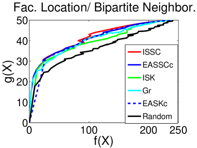
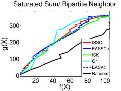
Figure 3: The two figures show the performance of the algorithms in the text on Problems 1 and 2 (in both cases, higher the better).

5 Experiments

In this section, we empirically compare the performance of the various algorithms discussed in this paper. We are motivated by the speech data subset selection application [30, 33, 21] with the submodular function $f$ encouraging limited vocabulary while $g$ tries to achieve acoustic variability. A natural choice of the function $f$ is a function of the form $|\Gamma(X)|$, where $\Gamma(X)$ is the neighborhood function on a bipartite graph constructed between the utterances and the words [33]. For the coverage function $g$, we use two types of coverage: one is a facility location function

$$g_{1}(X)=\sum_{i\in V}\max_{j\in X}s_{ij}$$ (43)

while the other is a saturated sum function

$$g_{2}(X)=\sum_{i\in V}\min\{\sum_{j\in X}s_{ij},\alpha\sum_{j\in V}s_{ij}\}.$$ (44)

Both these functions are defined in terms of a similarity matrix $\mathbf{S}=\{s_{ij}\}_{i,j\in V}$, which we define on the TIMIT corpus [9], using the string kernel metric [41] for similarity. Since some of our algorithms, like the Ellipsoidal Approximations, are computationally intensive, we restrict ourselves to $50$ utterances.

We compare our different algorithms on Problems 1 and 2 with $f$ being the bipartite neighborhood and $g$ being the facility location and saturated sum respectively. Since the primal and dual variants of the submodular set cover problem are similar, we just use the primal variants of ISSC and EASSC. Furthermore, in our experiments, we observe that the neighborhood function $f$ has a curvature $\kappa_{f}=1$. Thus, it suffices to use the simpler versions of algorithm EA (i.e., algorithm EASSCc and EASKc). The results are shown in Figure 3. We observe that on the real-world instances, all our algorithms perform almost comparably. This implies, moreover, that the iterative variants, viz. Gr, ISSC and ISK, perform comparably to the more complicated EA-based ones, although EASSC and EASK have better theoretical guarantees. We also compare against a baseline of selecting random sets (of varying cardinality), and we see that our algorithms all perform much better. In terms of the running time, computing the Ellipsoidal Approximation for $|\Gamma(X)|$ with $|V|=50$ takes about $5$ hours while all the iterative variants (i.e., Gr, ISSC and ISK) take less than a second. This difference is much more prominent on larger instances (for example $|V|=500$).

6 Discussions and related work

In this paper, we propose a unifying framework for problems 1 and 2 based on suitable surrogate functions. We provide a number of iterative algorithms which are very practical and scalable (like Gr, ISK and ISSC), and also algorithms like EASSC and EASK, which though more intensive, obtain tight approximation bounds. Finally, we empirically compare our algorithms, and show that the iterative algorithms compete empirically with the more complicated and theoretically better approximation algorithms.

To our knowledge, this paper provides the first general framework of approximation algorithms for Problems 1 and 2 for monotone submodular functions $f$ and $g$. A number of papers, however, investigate related problems and approaches. For example, [8] investigates an exact algorithm for solving problem 1, with equality instead of inequality. However, since problem 1 subsumes the problem of minimizing a monotone submodular function subject to a cardinality equality constraint, and is hence NP hard [36]. Hence this algorithm in the worst case, must be exponential. Furthermore, a similar problem was considered in [25] with one specific instance of a function $f$, which is not submodular. They also use, a considerably different algorithm. Also, an algorithm equivalent to the first iteration of ISSC was proposed in [46, 5] and ISSC not only generalizes this, but we also provide a more explicit approximation guarantee (we provide an elaborate discussion on this in the section describing ISSC). We also point out that, a special case of SCSK was considered in [29], with $f$ being submodular, and $g$ modular (we called this the submodular span problem). The authors there use an algorithm very similar to Algorithm 2, to convert this problem into an instance of minimizing a submodular function subject to a knapsack constraint, for which they use the algorithm of [43]. Unfortunately, the algorithm of [43] does not scale very well. Our algorithms for this problem, on the other hand, would continue to scale very well in practice.

Similarly, a number of approximation algorithms have been shown for Problem 0 [14, 37, 22]. The algorithms in [14, 37] are scalable and practical, but lack theoretical guarantees. The algorithm of [22] though exact, employs a branch and bound technique which is often inefficient in practice (the timing analysis from [22] also depicts that). These facts are not surprising, since problem 0 is not only NP hard but also inapproximable. Moreover, these algorithms are not comparable to ours, since we directly model the hard constraints and our bicriteria results give worst-case bounds on the deviation from the constraints and the optimal solution. This is often important, since there are hard constraints in many practical applications (in the form of power constraints, or budget constraints). Casting it as Problem 0, however, no longer has guarantees on the deviation from the constraints.

For future work, we would like to empirically evaluate our algorithms on many of the real world problems described above, particularly the limited vocabulary data subset selection application for speech corpora, and the machine translation application.

Acknowledgments: Special thanks to Kai Wei and Stefanie Jegelka for discussions, to Bethany Herwaldt for going through an early draft of this manuscript and to the anonymous reviewers for useful reviews. This material is based upon work supported by the National Science Foundation under Grant No. (IIS-1162606), a Google and a Microsoft award, and by the Intel Science and Technology Center for Pervasive Computing.

References

- [1] A. Atamtürk and V. Narayanan. The submodular knapsack polytope. Discrete Optimization, 2009.
- [2] Y. Boykov and M. Jolly. Interactive graph cuts for optimal boundary and region segmentation of objects in n-d images. In ICCV, 2001.
- [3] M. Conforti and G. Cornuejols. Submodular set functions, matroids and the greedy algorithm: tight worst-case bounds and some generalizations of the Rado-Edmonds theorem. Discrete Applied Mathematics, 7(3):251–274, 1984.
- [4] W. H. Cunningham. Decomposition of submodular functions. Combinatorica, 3(1):53–68, 1983.
- [5] H. Du, W. Wu, W. Lee, Q. Liu, Z. Zhang, and D.-Z. Du. On minimum submodular cover with submodular cost. Journal of Global Optimization, 50(2):229–234, 2011.
- [6] U. Feige. A threshold of ln n for approximating set cover. Journal of the ACM (JACM), 1998.
- [7] U. Feige, V. Mirrokni, and J. Vondrák. Maximizing non-monotone submodular functions. SIAM J. COMPUT., 40(4):1133–1155, 2011.
- [8] S. Fujishige. Submodular functions and optimization, volume 58. Elsevier Science, 2005.
- [9] J. Garofolo, F. Lamel, L., J. W., Fiscus, D. Pallet, and N. Dahlgren. Timit, acoustic-phonetic continuous speech corpus. In DARPA, 1993.
- [10] G. Goel, C. Karande, P. Tripathi, and L. Wang. Approximability of combinatorial problems with multi-agent submodular cost functions. In FOCS, 2009.
- [11] M. Goemans, N. Harvey, S. Iwata, and V. Mirrokni. Approximating submodular functions everywhere. In SODA, pages 535–544, 2009.
- [12] A. Guillory and J. Bilmes. Interactive submodular set cover. In ICML, 2010.
- [13] A. Guillory and J. Bilmes. Simultaneous learning and covering with adversarial noise. In ICML, 2011.
- [14] R. Iyer and J. Bilmes. Algorithms for approximate minimization of the difference between submodular functions, with applications. In UAI, 2012.
- [15] R. Iyer and J. Bilmes. The submodular Bregman and Lovász-Bregman divergences with applications. In NIPS, 2012.
- [16] R. Iyer, S. Jegelka, and J. Bilmes. Mirror descent like algorithms for submodular optimization. NIPS Workshop on Discrete Optimization in Machine Learning (DISCML), 2012.
- [17] R. Iyer, S. Jegelka, and J. Bilmes. Curvature and Optimal Algorithms for Learning and Minimizing Submodular Functions . In NIPS, 2013.
- [18] R. Iyer, S. Jegelka, and J. Bilmes. Fast semidifferential based submodular function optimization. In ICML, 2013.
- [19] S. Jegelka and J. Bilmes. Submodularity beyond submodular energies: coupling edges in graph cuts. In Computer Vision and Pattern Recognition (CVPR), 2011.
- [20] S. Jegelka and J. A. Bilmes. Submodularity beyond submodular energies: coupling edges in graph cuts. In CVPR, 2011.
- [21] S. Jegelka, H. Lin, and J. Bilmes. On fast approximate submodular minimization. In NIPS, 2011.
- [22] Y. Kawahara and T. Washio. Prismatic algorithm for discrete dc programming problems. In NIPS, 2011.
- [23] H. Kellerer, U. Pferschy, and D. Pisinger. Knapsack problems. Springer Verlag, 2004.
- [24] A. Krause and C. Guestrin. A note on the budgeted maximization on submodular functions. Technical Report CMU-CALD-05-103, Carnegie Mellon University, 2005.
- [25] A. Krause, C. Guestrin, A. Gupta, and J. Kleinberg. Near-optimal sensor placements: Maximizing information while minimizing communication cost. In IPSN, 2006.
- [26] A. Krause, B. McMahan, C. Guestrin, and A. Gupta. Robust submodular observation selection. Journal of Machine Learning Research (JMLR), 9:2761–2801, 2008.
- [27] A. Krause, A. Singh, and C. Guestrin. Near-optimal sensor placements in Gaussian processes: Theory, efficient algorithms and empirical studies. JMLR, 9:235–284, 2008.
- [28] A. Kulik, H. Shachnai, and T. Tamir. Maximizing submodular set functions subject to multiple linear constraints. In SODA, 2009.
- [29] H. Lin. Submodularity in Natural Language Processing: Algorithms and Applications. PhD thesis, University of Washington, Dept. of EE, 2012.
- [30] H. Lin and J. Bilmes. How to select a good training-data subset for transcription: Submodular active selection for sequences. In Interspeech, 2009.
- [31] H. Lin and J. Bilmes. Multi-document summarization via budgeted maximization of submodular functions. In NAACL, 2010.
- [32] H. Lin and J. Bilmes. A class of submodular functions for document summarization. In The 49th Meeting of the Assoc. for Comp. Ling. Human Lang. Technologies (ACL/HLT-2011), Portland, OR, June 2011.
- [33] H. Lin and J. Bilmes. Optimal selection of limited vocabulary speech corpora. In Interspeech, 2011.
- [34] L. Lovász. Submodular functions and convexity. Mathematical Programming, 1983.
- [35] R. C. Moore and W. Lewis. Intelligent selection of language model training data. In Proceedings of the ACL 2010 Conference Short Papers, pages 220–224. Association for Computational Linguistics, 2010.
- [36] K. Nagano, Y. Kawahara, and K. Aihara. Size-constrained submodular minimization through minimum norm base. In ICML, 2011.
- [37] M. Narasimhan and J. Bilmes. A submodular-supermodular procedure with applications to discriminative structure learning. In UAI, 2005.
- [38] G. Nemhauser and L. Wolsey. Best algorithms for approximating the maximum of a submodular set function. Mathematics of Operations Research, 3(3):177–188, 1978.
- [39] E. Nikolova. Approximation algorithms for offline risk-averse combinatorial optimization, 2010.
- [40] C. Rother, T. Minka, A. Blake, and V. Kolmogorov. Cosegmentation of image pairs by histogram matching-incorporating a global constraint into MRFs. In CVPR, volume 1, pages 993–1000. IEEE, 2006.
- [41] J. Rousu and J. Shawe-Taylor. Efficient computation of gapped substring kernels on large alphabets. Journal of Machine Learning Research, 6(2):1323, 2006.
- [42] M. Sviridenko. A note on maximizing a submodular set function subject to a knapsack constraint. Operations Research Letters, 32(1):41–43, 2004.
- [43] Z. Svitkina and L. Fleischer. Submodular approximation: Sampling-based algorithms and lower bounds. In FOCS, pages 697–706, 2008.
- [44] V. V. Vazirani. Approximation algorithms. springer, 2004.
- [45] J. Vondrák. Submodularity and curvature: the optimal algorithm. RIMS Kokyuroku Bessatsu, 23, 2010.
- [46] P.-J. Wan, D.-Z. Du, P. Pardalos, and W. Wu. Greedy approximations for minimum submodular cover with submodular cost. Computational Optimization and Applications, 45(2):463–474, 2010.
- [47] L. A. Wolsey. An analysis of the greedy algorithm for the submodular set covering problem. Combinatorica, 2(4):385–393, 1982.