Simple Multi-Party Set Reconciliation

Abstract

Many distributed cloud-based services use multiple loosely consistent replicas of user information to avoid the high overhead of more tightly coupled synchronization. Periodically, the information must be synchronized, or reconciled. One can place this problem in the theoretical framework of set reconciliation: two parties $A_{1}$ and $A_{2}$ each hold a set of keys, named $S_{1}$ and $S_{2}$ respectively, and the goal is for both parties to obtain $S_{1}\cup S_{2}$. Typically, set reconciliation is interesting algorithmically when sets are large but the set difference $|S_{1}-S_{2}|+|S_{2}-S_{1}|$ is small. In this setting the focus is on accomplishing reconciliation efficiently in terms of communication; ideally, the communication should depend on the size of the set difference, and not on the size of the sets.

In this paper, we extend recent approaches using Invertible Bloom Lookup Tables (IBLTs) for set reconciliation to the multi-party setting. There are three or more parties $A_{1},A_{2},\ldots,A_{n}$ holding sets of keys $S_{1},S_{2},\ldots,S_{n}$ respectively, and the goal is for all parties to obtain $\cup_{i}S_{i}$. Whiel this could be done by pairwise reconciliations, we seek more effective methods. Our general approach can function even if the number of parties is not exactly known in advance, and with some additional cost can be used to determine which other parties hold missing keys.

Our methodology uses network coding techniques in conjunction with IBLTs, allowing efficiency in network utilization along with efficiency obtained by passing messages of size $O(|\cup_{i}S_{i}-\cap_{i}S_{i}|)$. By connecting reconciliation with network coding, we can provide efficient reconciliation methods for a number of natural distributed settings.

Key words: set reconciliation; synchronization; multi-party; network coding; hashing; sketching.

1 Introduction

As users migrate information to cloud storage, the burden of reliability moves to the cloud provider. Thus many cloud vendors such as Amazon [13] and Azure [8] use multiple loosely consistent replicas of user information because of the high overhead of keeping replicas synchronized at all times. Further, users often retain copies of their information on laptops, tablets, phones and Personal Digital Assistants (PDAs); these devices are often disconnected from cloud storage and thus can diverge from the corresponding copies in the cloud. The situation naturally grows even more complicated when multiple users have access to information, because the number of replicas can increase with the number of users. Periodically, however copies of information objects must be synchronized or reconciled. One can also view the need for reconciliation at a higher level, such as for loosely consistent replicas of large databases that may be used for availability by information providers.

This paper focuses on the basic problem of set reconciliation. In the 2-party setting, two parties $A_{1}$ and $A_{2}$ respectively have (usually very similar) sets $S_{1}$ and $S_{2}$, and want to reconcile so both have $S_{1}\cup S_{2}$. Our major contribution is to extend the recent approach to set reconciliation for two parties using Invertible Bloom Lookup Tables (IBLTs) to the multi-party setting, where there are three or more parties holding sets $S_{1},S_{2},S_{3},\ldots,S_{n}$, and the goal is for all parties to obtain $\cup_{i}S_{i}$. This could of course be done by pairwise reconciliations, but we seek more efficient methods. We first extend the IBLT approach, showing that in the multi-part setting we can reconcile using messages of size $O(|\cup_{i}S_{i}-\cap_{i}S_{i}|)$. This generalizes results from the two-party setting, where the information theoretic goal has been to send information close to the size of the set difference, rather than sending information proportional to the size of the sets, as generally the set difference is very small compared to the set sizes. Our approach has other advantages, including that one does not need to know the number of parties in advance. Our main approach here, related to network coding, is to think of the information stored in the IBLT as corresponding to vectors over a suitable finite field instead of the binary vectors used in previous work.

We further show that our methodology allows using further network coding techniques in conjunction with IBLTs, providing additional efficiency in terms of network utilization. By connecting reconciliation with network coding, we can provide more efficient reconciliation methods that apply to a number of natural distributed computing problems. For example, using recent results from gossip algorithms, we show that multi-party set reconciliation over a network with $n$ nodes can be done in $O(\phi^{-1}\log n)$ rounds of communication with IBLTs, where $\phi$ is the conductance of the network.

While our work can be seen as a specific example of a linear sketch that has a natural affinity to the network coding approach, we believe it suggests that other linear sketch-based data structures may also find expanded use by combining them with ideas from network coding.

1.1 Potential Applications and Related Work

The use of IBLTs for distributed synchronization has already been proposed for specific applications. For example, recently the Bitcoin community has considered using IBLTs for scalable synchronization of transactions [1, 20]. Multi-party variations would be potentially useful in the Bitcoin setting, where multiple parties may need to track transactions.

In the setting of data centers, as shown in the survey of Bailis and Kingsbury [2], network errors abound in cost-effective large-scale environments. Thus, even if we attempt to keep multiple copies of data synchronized, the synchronization will periodically fail along with the network, leaving the problem of reconciling the differences.

As related work, we note that a different generalization of the set reconciliation problems, to settings where a certain type of approximate reconciliation is desired, was recently considered in the database community [9]. However, that work focuses on the setting of two parties, leaving the question of scaling to many parties open.

Another related model for problems on distributed data is that of distributed tracking (see e.g. [23]). Our problem differs from distributed tracking in two respects: we focus on exact computation (with an arbitrarily small error probability), and we focus on periodic, as opposed to continuous, computation of the joint function.

Several further specific applications for set difference structures are given in [17], including peer-to-peer transactions, deduplication, partition healing, and synchronizing parallel activations (e.g., of independent crawlers of a search engine). They also discuss why logging as an alternative may have disadvantages in multiple contexts; an example they provide is for “hot” data items that are written often and may therefore be in the log multiple times. We refer the reader to this paper for more information on these examples. Multi-party variations of IBLT-based synchronization methods could enhance their desirability in these applications when multiple parties naturally arise. In synchronizing parallel activations, for instance, several agents in a distributed system could be gathering information into local databases in a redundant fashion for near-optimal accuracy in the collection process, and then need to reconcile these local databases into a synchronized whole.

1.2 Background

We briefly summarize known results for the historically common setting of two parties with direct communication. Consider two parties $A_{1}$ and $A_{2}$ with sets $S_{1}$ and $S_{2}$ of keys from a universe $U$. An important value is the size of the set difference between $S_{1}$ and $S_{2}$, denoted by $d=|S_{1}-S_{2}|+|S_{2}-S_{1}|=|(S_{1}\cup S_{2})-(S_{1}\cap S_{2})|$. In this setting there are communication-efficient algorithms when $d$, or a good approximate upper bound for $d$, is known. Hence, in some algorithms for set reconciliation, there are two phases: in a first phase a bound on $d$ is obtained, which then drives the second phase of the algorithm, where reconciliation occurs. See [28] for further discussion on this point.

One previous approach to set reconciliation uses characteristic polynomials, in a manner reminiscent of Reed-Solomon codes [28]. Treating keys as values, $A_{1}$ considers the characteristic polynomial

$$\chi_{S_{1}}(Z)=\prod_{x_{i}\in S_{1}}(Z-x_{i}),$$

and similarly $A_{2}$ considers $\chi_{S_{2}}(Z)$. Observe that in the rational function

$$\frac{\chi_{S_{1}}(Z)}{\chi_{S_{2}}(Z)},$$

common terms cancel out, leaving a rational function in $Z$ where the sums of the degrees of the numerator and denominator is at most $d$. The rational function can be determined through interpolation by evaluating the function at $d+1$ points over a suitably large field; hence, if $A_{1}$ sends the value of $\chi_{S_{1}}(Z)$ at $d+1$ points and $A_{2}$ sends the value of $\chi_{S_{2}}(Z)$ at the same (pre-chosen) $d+1$ points, then the two parties can reconcile their set difference. If the range can be embedded in a field of size $q$, the total number of bits sent in each direction would be approximately $(d+1)\lceil\log_{2}q\rceil$. Note that this takes $O(d^{3})$ operations using standard Gaussian elimination techniques. Similar ideas underlie similar results by Juels and Sudan [24]; these ideas can be extended to use other codes, such as BCH codes, with various computational tradeoffs [15].

Recent methods for set reconciliation have centered on using randomized data structures, such as the Invertible Bloom Filter or the related but somewhat more general Invertible Bloom Lookup Table (IBLT) [16, 17, 19]. For our purposes, the Invertible Bloom Lookup Table is a randomized data structure storing a set of keys that supports insertion and deletion operations, as well as a listing operation that lists the keys in the structure. We review the use of IBLTs for 2-party set reconciliation in Section 2. The main effect of using IBLTs is that one can give up a small constant factor in the data transmitted to obtain speed and simplicity that is desirable for many implementations. 2-party reconciliation using IBLTs can generally be done in linear time, using primarily hashing and XOR operations. As we show in this paper, the use of IBLTs can also be extended to multi-party reconciliation.

While the theory set reconciliation among two parties has been widely studied, there appears to be no substantial prior work (that we are aware of) specifically examining the theory of multi-party reconciliation schemes, although the question of how to implement them was raised in [29]. Special cases, such as rumor spreading (see, e.g., [10, 12, 14, 18, 22, 34]), where one (or more) parties have a single key to share with everyone, have been studied, however.

In more practical work, reconciliation among multiple parties has been studied, often in the context of distributed data distribution, using such techniques as erasure coding and Bloom filters to enhance performance or reduce the overall amount of data transferred (e.g., [7, 26, 33, 17]). However, these works are also based on pairwise reconciliation, and some do not attempt to achieve data transmission proportional to the size of the set difference, which is our goal here. The work closest to ours is [17], which also uses Invertible Bloom Filters, but is focused on pairwise reconciliation.

2 Review: The 2-Party Setting

We review 2-party set reconciliation, using the framework of the Invertible Bloom Filter/ Invertible Bloom Lookup Table (IBLT) [16, 17, 19]. More concretely, we first describe an IBLT and its use for set reconciliation. IBLTs store keys, which here we will think of as fixed-length bit strings. An IBLT is designed with respect to a threshold number of keys, $t$, so that listing will be successful with high probability if the actual number of keys in the structure at the time of a listing operation is less than or equal to $t$. An IBLT ${\cal B}$ consists of a lookup table $T$ of $m$ cells initialized with all entries set to 0, where $m$ is $O(t)$, and the constant factor in the order notation is generally small (between 1 and 2) depending on the parameters chosen. Like a standard Bloom filter, an IBLT uses a set of $k$ random hash functions, $h_{1}$, $h_{2}$, $\ldots$, $h_{k}$, to determine where keys are stored. For simplicity, we assume random hash functions here, and for technical reasons we assume that the hashes of each key yield distinct locations; hence the $k$ hashes yield a uniform subset of $k$ distinct cells from the $m\choose k$ possibilities. Alternatively, this could easily be accomplished, for instance, by splitting the table into $k$ subtables and having the $i$th hash function choose a location independently and uniformly at random in the $i$th subtable, which would not asymptotically change the thresholds [4].

The IBLT uses a hash function $H$ that maps keys to hash values in a large range of size $q$ (where $q$ will be chosen later to bound the probability of error). The IBLT uses a hash function $H$ that maps keys to hash values in a large range of size $q$ (where $q$ is a power of 2 that will be chosen later to bound the probability of error). For the purpose of this paper we assume that $H$ is a fully random hash function. Each key $x$ is placed into cells $T[h_{1}(x)]$, $T[h_{2}(x)],\dots,T[h_{k}(x)]$, where again $T$ is the lookup table that represents the IBLT, as follows.

Each cell $T[i]$ contains an ordered pair

$$(\textsf{keySum},\textsf{keyhashSum})\enspace.$$

The keySum field is the XOR of all the keys that have been mapped to this cell, and hence must be the size of the keys (in bits). The keyhashSum field is the XOR of all the hash values $H(x)$ that have been mapped to this cell, and hence must be the size of the hash $H$ of the keys (in bits). Note that insertion and deletion is the same operation, as a deletion operation reverses an insertion. Hence it is possible to delete a key without it first being inserted.

Set reconciliation using IBLTs

The above structure yields a set reconciliation algorithm. Consider two parties Angel and Buffy (or $A_{1}$ and $A_{2}$). Angel places his keys into an IBLT, as does Buffy. They are assumed to share the hash functions $h_{i}$ and $H$ according to some prior arrangement. They transfer their corresponding IBLTs, and each then deletes their own keys from the transferred IBLTs. Each IBLT then contains the set difference, and the set difference is recovered using the listing process. Alternatively, since deleting and inserting both correspond to XOR operations, we can say that the parties take the sum of the IBLTs, by which we simply mean that for each field in each cell, the corresponding values are summed via the bitwise XOR operation. As long as the set difference size $d$ is less than the threshold $t$, recovery will occur with high probability (in $t$).

As it will help us subsequently, we describe how the listing process functions. Listing the contents of IBLTs uses a “peeling process”. Peeling here corresponds to finding a cell with exactly one key contained in it, after the insertion/deletion steps by Angel and Buffy have effectively removed keys that appear in both sets. To find a cell with one key, we check the keySum field using keyhashSum. That is, if the keySum field contains a value $z$, we check whether keyhashSum contains the value $H(z)$. If $z$ is the actual key contained in the cell, then $H(z)$ will indeed appear in the keyhashSum field. If the keySum field contains the XOR of several keys, then (under our assumption of random hash values for $H$) there will be a false positive with probability only $1/q$ where $q$ is the size of the range of hash values for $H$. Let us temporarily assume that there are no false positives.

Once we have a cell with a single recoverable key $z$, we can remove $z$ from the structure by computing $h_{i}(z)$ for all $i$ and deleting $z$ from the corresponding cells using exclusive-or operations to update the keySum and keyhashSum fields. Removing a key from the structure may yield new keys that can be recovered. This peeling process has been used in a variety of contexts, such as in erasure-corrected codes [27]. The peeling process may also fail simply because at some point there may not be any available cell with only a single recoverable key. It can be shown that recovery occurs with high probability, assuming a suitably-sized IBLT is used [19, 27, 30]. Specifically, the process of peeling corresponds to finding what is known as the 2-core – the maximal subgraph where all vertices are adjacent to at least two hyperedges – on a hypergraph where cells correspond to vertices and each key $x$ corresponds to the hyperedge $\{h_{1}(x),\dots,h_{k}(x)\}$. When $k$ is a constant, the peeling process yields an empty $k$-core with high probability whenever the table size $m$ satisfies $m>(c_{k}+\epsilon)t$ for a constant threshold coefficient $c_{k}$ and constant $\epsilon>0$. As noted in [19], the threshold coefficients, given in Table 1, are close to 1. (Again, they can be made closer to 1 if desired using irregular hypergraph constructions [19, 31].)

$k$	3	4	5	6	7
$c_{k}$	1.222	1.295	1.425	1.570	1.721

Table 1: Threshold coefficients for the 2-core rounded to four decimal places.

The following theorem, paraphrased from [19], provides the probabilistic bounds on the failure probability of the peeling process.

Theorem 2.1

As long as we choose $m>(c_{k}+\epsilon)t$ for some $\epsilon>0$, the listing operation (not counting the separate probability of false positives from keyhashSum) fails with probability $O(t^{-k+2})$.

We now bound the running time for peeling and error probability from false positives from the keyhashSum field. Given an IBLT to peel, we can start by taking a pass over the $O(t)$ cells of the IBLT to find cells where the keySum field contains a value $z$ and the keyhashSum contains the value $H(z)$. We keep a list of such cells and start the peeling with these cells. As we peel a cell we update the keySum and keyhashSum fields of other cells. As we proceed through the list, we might encounter cells that have already been peeled — these are simply ignored. Also, while peeling we test cells that we delete keys from to see if now the keySum and keyhashSum fields match, in which case the cell can be added to the list of cells to peel. Overall this process clearly takes $O(t)$ time (constant time per peeling operation), and there are $O(t)$ times that we compare keySum and keyhashSum fields within a cell, each of which can yield a false positive with probability $1/q$. Under a worst-case assumption that any such error would cause a listing failure, this gives a total error probability of at most $O(t/q)$ caused by a false positive in the keyhashSum field. We can choose $q$ according to our desired error bound.

Adapting to the set difference size

If we have an upper bound on $d$, we can use this upper bound as the value $t$ for the IBLT, and apply Theorem 2.1. We henceforth assume that an upper bound within a (small) constant factor of $d$ is available throughout this work, as finding an upper bound is essentially an orthogonal problem. Without an upper bound on $d$, some additional work may need to be done, as explored in for [17, 28]; we summarize these results and offer other alternatives as they apply here. Both of [17, 28] suggest approaches that correspond to repeated doubling; if the IBLT size is not sufficient, so that decoding is unsuccessful, then start over with larger IBLTs. Another option is to double the IBLT size by adding one additional lower-order bit to each hash value. Then it suffices to send every odd-numbered cell of the IBLT arrays, since the even-numbered cells can be found by subtraction from the old IBLT. In this way, the total number of cells transmitted is the same as if the final IBLT had been transmitted initially. If the set difference is small but still a constant fraction of the union of the set sizes, then using min-wise independence or related techniques [5, 11] to approximate the set difference may be suitable. Finally, one might incrementally improve the IBLT. If each hash function is assigned its own subarea of cells (as is often how Bloom filters are implemented to allow parallel lookups into the structure [6], and as noted in [19] is advantageous for IBLTs), then the parties can incrementally add another hash function by sending additional information corresponding to the subarea for the additional hash function.

Keeping count

Finally, the IBLT can also contain an optional count field, which gives a count for the number of keys in a cell. We can increase the count by 1 on insertion, and decrease it by 1 on deletion. With a count field, a cell can contain a recoverable key only if the count is 1 or $-1$. (From Angel’s point of view, after deleting his keys from Buffy’s IBLT, when the count is $-1$, it could correspond to a cell containing a key of his that Buffy does not have.) Note, however, a count of 1 or $-1$ does not necessarily correspond to a cell with a recoverable key. For example, if Angel has two keys Buffy does not hold that hash to the same cell, and Buffy has one key that Angel does not have that hashes to the same cell, then after taking the difference of the IBLTs the count will be 1 but there will be as sum of three keys in the cell. The count field can be useful for implementation and assists by acting like the sum of another trivial “hash” value for the key (all keys hash to 1), but it does not replace the keyhashSum field.

Abstraction

At an abstract level, we can view the 2-party setting as follows. We desire a linear sketch (over an appropriate field) taken on sets of keys with the following properties. Let $f(S)$ denote the sketch of the set $S$. We desire

• $f((S_{1}\cup S_{2})-(S_{1}\cap S_{2}))=f(S_{1})\oplus f(S_{2})$;

• a set $X$ can be efficiently extracted from $f(X)$ under suitable conditions, which here means that $X$ is sufficiently small;

• the size of the sketch is small, which here means that that if we want to recover $(S_{1}\cup S_{2})-(S_{1}\cap S_{2})$ then the sketch size is $O(|(S_{1}\cup S_{2})-(S_{1}\cap S_{2})|)$.

We have focused our description on IBLTs as it is a sketch with the required properties. For multi-party reconciliation, we now show that IBLTs can be extended by working over an appropriate field to ensure that with multiple sets $S_{1},S_{2},\ldots,S_{n}$, we have $f(\cup_{i}S_{i}-\cap_{i}S_{i})=\sum_{i}f(S)$, while still maintaining suitable extraction and size properties.

3 The 3-Party Setting

We now describe the extension of IBLTs to provide set reconciliation for three parties. Starting with the 3-party setting allows us to demonstrate the key ideas behind this approach and explore its capabilities; we then examine how these extensions can be used beyond three parties.

To start each of our three parties – Angel, Buffy, and Cordelia (or $A_{1}$, $A_{2}$, and $A_{3}$) – inserts keys and hashes of keys into the IBLT. (For now, we will not use a count field.) However, in this setting both the keys and the hashes of keys are mapped injectively to values in $(\mathbb{F}_{3})^{b}$ for an appropriate $b$. The particular way of mapping to $(\mathbb{F}_{3})^{b}$ does not matter — we could interpret the key and hash values as number base 3 (at the cost of converting to base 3), or (at the cost of some space) we could interpret the vector of bits of the key or hash value as a vector in $(\mathbb{F}_{3})^{b}$. Now, instead of using XOR in our insertion operation – which is equivalent to treating keys as $b$-bit elements of $(\mathbb{F}_{2})^{b}$ – we move to $(\mathbb{F}_{3})^{b}$ (treating keys as sequences of $b$ trits; similarly, hash values are sequences of trits, perhaps of a different length). The three IBLT data structures are combined by summing each of the keySum fields for each cell, as well as summing the keyhashSum fields for each cell, where the sums are sums of elements in $(\mathbb{F}_{3})^{b}$. To begin, let us ignore the issues of the underlying network and assume that all parties obtain all 3 IBLTs.

Any key that appears in all three sets is canceled out of keySum by the summation, and similarly the summation of the three hashes of the key is canceled out of keyhashSum. Hence the number of keys existing in the IBLT after this cancellation is $|\cup_{i}S_{i}-\cap_{i}S_{i}|$. If a key $x$ is found in the keySum field and a matching $H(x)$ is in the keyhashSum field, the key is recovered and removed by subtracting $x$ and $H(x)$ (or equivalently, adding in $2x$ and $2H(x)$ in the appropriate fields). However, some of these keys may appear duplicated in the IBLT; for example, if Angel and Buffy have a key $x$ but Cordelia does not, then the sum of the 3 IBLTs may have a cell containing the value $2x$ in the keySum field and $2H(x)$ in the keyhashSum field. We therefore must further modify our method of recovery. If we see a value $z$ in the keySum field, we must check whether the value $H(z)$ appears in the keyhashSum field, but we must also check whether $2H(z/2)$ appears in the keyhashSum field, in which case we treat it is a verification of $z/2$ as the key. This increases our error rate due to false positives from keyhashSum by at most a factor of two, which is still $O(t/q)$. We note that we could reduce this error rate by instead keeping a count field, which would tell us which one of the two cases above may apply. Also, we note that when removing this key from the IBLT, each cell it is hashed to would then have to remove two copies of the key.

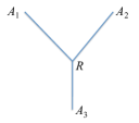
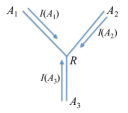
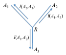
Figure 1: Set reconciliation with network coding. The relay $R$ receives an IBLT from each party, and sends back to each party the sum of the other parties’ IBLTs. Each party just needs to send and receive one message, improving on pairwise set reconciliation protocols. Alternatively, in the subfigure on the right, in a wireless setting the relay $R$ can broadcast the sum of all the IBLTs to all parties (denoted by dotted lines), reducing the number of messages further.

We emphasize that despite this difference, the IBLT listing process works in the same manner, and in particular has the same threshold size for successful listing. This is because a key is recovered exactly when a key is the only key hashed to a cell; the multiplicity of that key within the cell does not affect the listing process. As the IBLT recovery works in the same manner as in the 2-party case, we have the following theorem, based on Theorem 2.1.

Theorem 3.1

Consider a 3-party reconciliation using IBLTs with $k$ hash functions and a range of $q$ values in the keyhashSum field. As long as we choose $m>(c_{k}+\epsilon)t$ for some $\epsilon>0$, and $t\geq|\cup_{i}S_{i}-\cap_{i}S_{i}|$, the 3-way reconciliation protocol fails with probability $O(t^{-k+2}+t/q)$.

The 3-party protocol uses $m$ cells, which contain the key and a hash. As long as the keys are sufficiently large so that the hash is relatively small compared to the keys, the constant factor from overhead will be small. For 64-bit keys and 32-bit hashes, for example, the total overhead should be less than a factor of 2 for $k=3,4$, and less than a factor of 3 for $k$ up to 7. In many settings, keys or associated stored values can be significantly longer than 64 bits and the overhead will be much smaller.

3.1 Useful Extensions

Note that from this process each party can determine the number of other parties (1 or 2) that hold a key they do not possess. It is not hard to add some additional information so that each party can determine which other party holds the key. For example, we could add a 3-bit IDs field to each cell; each time $A_{i}$ adds (or removes) a key from the IBLT it would toggle the $i$th bit. Hence the $i$th bit of the IDs field would record the parity of the number of keys that $A_{i}$ has added to the cell. Recall that when we recover a key from the cell, it should be the only key in that cell; hence, the bits set to 1 in the IDs field correspond to the parties that hold that key. (We note that, in fact, having a modulo 3 counter, and having $A_{i}$ add $i$ to that counter when adding a key, would in fact suffice in this case; the details are left to the reader. Our description here generalizes more readily.)

Another reasonable question one might ask is if one party drops out of the protocol, can the remaining two parties still reconcile their sets. The answer is yes. Suppose Cordelia does not participate, so that only Angel and Buffy swap IBLTs. In this case, when combining IBLTs, Angel adds his own IBLT twice (or simply multiples every entry in his IBLT by 2 initially), and similarly for Buffy. That is, each participating party can simply act as though they were two parties with the same set. This guarantees that any key shared by both parties appears 3 times in the IBLT and is canceled; the IBLT listing can be done as above. Note that a participating party must know the number of other participating parties, potentially requiring dropping parties to signal their dropping out in some way.

3.2 Combining with Network Coding

We have thus far assumed that all participating parties get all IBLTs, and hence it may not be clear that this approach is significantly advantageous when compared to simply performing pairwise reconciliations. However, significant advantages become clearer when we consider the transmission of IBLTs over a network. Because IBLTs are linear sketches, based solely on addition, linear network coding methods can be applied.

Specifically, suppose $A_{1}$, $A_{2}$, and $A_{3}$ are communicating over a network via a relay $R$. We emphasize that this is a simple setting for illustrative purposes.

In Figure 1 we let $I(A_{i})$ represent the IBLT for $A_{i}$, and similarly let $I(A_{i},A_{j})$ be the sum of the IBLTs for $A_{i}$ and $A_{j}$, and so on. If we sent $I(A_{1})$ to $A_{2}$ and $A_{3}$, even if the relay duplicates the IBLT it will have to cross 3 links, and similarly for the other two IBLTs. Hence, the total transmission cost will be 9 IBLTs worth of data. However, suppose as shown in Figure 1 that all the Bloom filters $I(A_{1}),I(A_{2})$, and $I(A_{3})$ are sent to the relay $R$, and $R$ then takes sums to send $I(A_{2},A_{3})$ to $A_{1}$, and similarly for the other parties. Now only 6 IBLTs worth of data need to be sent, saving 1/3 of the transmission cost. This savings is entirely similar to standard network coding techniques.

Indeed, in the wireless setting, we could instead have the relay $R$ broadcast the joint IBLT $I(A_{1},A_{2},A_{3})$ of all parties to all the parties, reducing the number of messages down to four. This approach is similar to the now well-known approach of using simple XOR-based network coding in wireless networks [25].

We note that, in this relay setting, instead of using an IBLT with entries over $(\mathbb{F}_{3})^{b}$, we could build up a joint IBLT using standard IBLTs by having the relay do more work. Given IBLTs $I(A_{1})$ and $I(A_{2})$, the relay could determine the set difference from the pair of IBLTs, and correspondingly add elements to one IBLT to create an IBLT for the union of the sets. Then on the arrival of $I(A_{3})$ the relay could again determine the set difference between $A_{1}\cup A_{2}$ and $A_{3}$ and use this to build an IBLT for $A_{1}\cup A_{2}\cup A_{3}$. This repeated decoding and encoding approach is used in [3]. However, this approach requires much more work from the relay, namely a full decoding for each newly received IBLT, which should be avoided in many settings. Our work shows, for the first time, that such additional work can naturally be avoided.

4 Generalizing to $n$ Parties

We now consider the generalization to $n$ parties. We use a field of characteristic $p$, where $p\geq n$, and we assume keys are mapped injectively (in an arbitrary way) into $(\mathbb{F}_{p})^{b}$, for some $b$. For convenience we simply take $p$ to be a prime here, so that keys are mapped to vectors of non-negative integers smaller than $p$, and sums are computed modulo $p$. (And similarly for hash values, for a possibly different $b$). For simplicity, the reader might think about $b=1$, so keys and hash values are mapped injectively to integers modulo $p$. For convenience we will assume multiplication and division modulo $p$ can be done in constant time; those who object to this assumption may add an appropriate $O(\log^{2}p)$ factor to the time bounds (although better bounds may be possible with specially chosen primes). Let $v_{i}$ denote the representation of $I(A_{i})$ as a vector as above.

For efficiency and to reduce the probability of a false positive when using the keyhashSum to verify the key value in the cell, we keep a counter modulo $p$ in the count field to track the count of the number of (copies of) keys hashed to a cell by all parties

We first state a general result that may not appear directly relevant at first blush. However, this form is useful in that it can be applied to more specific situations, including not only the straightforward generalization to $n$ parties, where we consider a sum of $n$ IBLTs, but also situations (motivated by randomized network coding) in which we are given two different linear combinations of IBLTs, and need to do set reconciliation. The condition under which set reconciliation succeeds is somewhat technical, and it is possible that some set $X$ of keys cannot be recovered. But as we will see, for the linear combinations of interest (such as random linear combinations) the probability that $X\neq\emptyset$ can be made small; in some settings (e.g., when a sum of IBLTs is obtained as in from a relay) the probability will be 0.

Theorem 4.1

Consider an $n$-party reconciliation using IBLTs with $k$ hash functions and a range of $q$ values in the keyhashSum field. Suppose we know two linear combinations (over $(\mathbb{F}_{p})^{b}$) $L_{1}=\sum_{i=1}^{n}\alpha_{i}v_{i}$ and $L_{2}=\sum_{i=1}^{n}\beta_{i}v_{i}$, as well as the sums of coefficients $\alpha=\sum_{i}\alpha_{i}\bmod p$ and $\beta=\sum_{i}\beta_{i}\bmod p$, where $\alpha_{i}\neq 0\bmod p$ for all $i$, and $\beta\neq 0\bmod p$. Let $X=\{x\in\cup_{i}S_{i}\;|\;\sum_{i}(\alpha_{i}+\gamma\beta_{i})1_{x\in S_{i}}\bmod p=0\}$, where $\gamma=-\alpha\beta^{-1}\bmod p$, and $1_{E}$ is an indicator random variable for the event $E$. As long as we choose $m>(c_{k}+\epsilon)t$ for some $\epsilon>0$, and $t\geq|\cup_{i}S_{i}-\cap_{i}S_{i}|$, then from $L_{1}$ and $L_{2}$ we can determine all keys from $(\cup_{i}S_{i}-\cap_{i}S_{i})-X$, with probability $1-O(t^{-k+2}+t/q)$.

Proof

If a key is present in all sets $S_{i}$ then it appears with coefficient $\alpha$ in $L_{1}$, and similarly it will appear with coefficient $\beta$ in $L_{2}$. From these we can form the combination of $L_{1}+\gamma L_{2}$, where as stated $\gamma=-\alpha\beta^{-1}\bmod p$. The coefficient of a key that is present in all sets $S_{i}$ is then 0 modulo $p$ and therefore the key is not present in the IBLT $L_{1}+\gamma L_{2}$. Unfortunately, the same is true for any key that appears exactly in sets $S_{j}$ for $j\in T$ when $T$ has the property that $\sum_{i\in T}(\alpha_{i}+\gamma\beta_{i})=0\bmod p$. All other keys can be found with the given probability using the IBLT recovery process. Note we assume the use of a count field that tracks the weighted multiplicity of the number of keys hashed to a cell modulo $p$ (that is, the sum of the coefficients of the keys hashed to that cell), so that only a single possible key value must be tested in a cell at any time. It is this use of the count field that limits the additional failure probability to $O(t/q)$.

We also remark that in the case where $\alpha=0$, the theorem also holds, but in fact there is no need for the second linear combination $L_{2}$ (as $\gamma=0$). In this case, a key present in all sets has a multiplicity that is $0\bmod p$, and $X$ corresponds those keys $x$ that appear exactly in sets $S_{j}$ for $j\in T$ where $T$ has the property that $\sum_{i\in T}\alpha_{i}=0\bmod p$.  

To see how Theorem 4.1 can be used, we first consider the basic case, where each party simply wants to find $\cup_{i}S_{i}-\cap_{i}S_{i}$. We first provide the argument without using the theorem, and then see how the theorem immediately implies the result. Let us assume that each party $A_{i}$ obtains the sum of all IBLTs $Z=\sum_{i}v_{i}$, and of course each party $A_{i}$ also has $S_{i}$ and hence $v_{i}$. If $p>n$, then after $A_{i}$ obtains the sum $Z$ of all IBLTs, it computes the sum $Z+(p-n)v_{i}$, essentially acting as $p-n+1$ parties with the same set. As before, this means that the contributions of keys appearing in all sets will cancel out. Each key not appearing in all sets will have an associated multiplicity of less than $n$ in $Z$ and hence less than $p$ in $Z+(p-n)v_{i}$ (regardless of whether the key is in $S_{i}$ or not). The algorithm can then for each cell examine the count $a$, the keySum $y$, and the keyhashSum $z$ to determine if $H(a^{-1}y)=a^{-1}z\bmod p$, which is true when the count $a$ corresponds to a single key. Hence, as before, each key not in all sets can be recovered using the IBLT recovery process with probability $1-O(t^{-k+2}+t/q)$. (For small $n$ one might choose not to use a count field; one could avoid keeping the count field and test all possible count values, that is try all values of $a$ from 1 to $p-1$. Or one can be slightly smarter; if $A_{i}$ contains a single $x\in S_{i}$ that hashes to that cell, then $A_{i}$ need only test the value of $a$ that satisfies $ax=y$, and if $A_{i}$ has $x\in S_{i}$ that hashes to that cell, then only $a$ values from $1$ to $n-1$ need to be tested.)

Alternatively, we see that this matches the setting of Theorem 4.1, with $L_{1}=Z$, $L_{2}=v_{i}$, and $\gamma=-n$. Computing $Z-nv_{i}=Z+(p-n)v_{i}\bmod p$ we see that the set $X$ must be empty, because as we argued above any key not in all sets has a count that is non-zero modulo $p$ in $Z+(p-n)v_{i}$. The result follows.

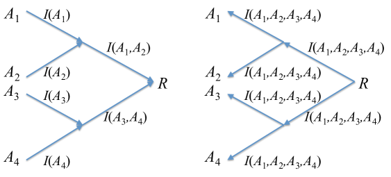
Figure 2: Set reconciliation example when the parties are connected by a communication tree, a common case in network communications.

4.1 Extensions

Several of our extensions from Section 3.1 hold in this framework as well. For example, with an $n$-bit IDs field one can track the parity of the number of keys in a cell for each of the $n$ parties, and thereby determine the parties that hold a recovered key. Also, if some parties do not participate, each participating party can simply add in additional copies of its own IBLT to arrange for cancellation if all participating parties hold a key. All that needs to be known for recovery is the number of participating parties.

In the case of $n$ parties connected through a relay node, we find that by passing IBLTs through the relay, we can arrange for $n$-party set reconciliation using $2n$ messages on a wired network and $n+1$ messages on a wireless network, where the relay broadcasts the sum of the IBLTs to all parties. This improves over the simplistic natural approach of using $n(n-1)$ point-to-point messages to compute all pairwise differences. However, it should be noted, the pairwise difference messages may in fact be smaller in size, since pairwise set differences may be smaller than the total set difference.

5 Network Coding and IBLTs

At a high level, our work thus far suggests that, by working over a suitable finite field, IBLTs can be naturally plugged in to linear network coding schemes to provide efficient set reconciliation mechanisms, where the message size corresponds (up to constant factors) to the generalized set difference. We believe this correspondence is indeed quite general, and while the broad nature of use and applications of network coding make it difficult to turn this statement into a theorem, we provide some sample applications.

5.1 Set Reconciliation on Trees

We first consider set reconciliation among $n$ parties, connected by a communication network that is a rooted tree with $E$ edges, known in advance. The parties are at the leaves of the tree. At each time step, each node in the tree can send a message to each of its neighbors. Let $P$ be the length of the longest path from a leaf to a root of the tree. We assume in what follows that keys are sufficiently large so that other overhead (e.g., the keyhashSum field) at most affects the total size by a constant factor, and that an upper bound on $|\cup_{i}S_{i}-\cap_{i}S_{i}|$ within a constant factor is known. We claim the following.

Theorem 5.1

Set reconciliation among $n$ parties on a rooted tree can be performed in $2P$ time steps with $2E$ total messages of size $O(|\cup_{i}S_{i}-\cap_{i}S_{i}|)$ with probability $1-O(t^{-k+2}+nt/q)$. Each non-leaf node in the network requires only $O(|\cup_{i}S_{i}-\cap_{i}S_{i}|)$ storage.

Proof

Each party constructs its IBLT, and sends it up the communication network to the root. Non-leaf nodes excluding the root combine all the IBLTs from leaves in their subtree, and pass them up to the root. The root gathers all the IBLTs and sends the union of them back down the communication tree. (See Figure 2.) Messages are of size $O(|\cup_{i}S_{i}-\cap_{i}S_{i}|)$, and each edge of the tree carries a single message in each direction. The IBLTs allow each party to recover all keys with probability $1-O(t^{-k+2}+t/q)$. This follows immediately from Theorem 4.1, as again we are in the setting where $L_{1}=\sum_{i}v_{i}$ and $L_{2}=v_{i}$. All of the IBLTs will be peeling the same set of keys, so the $O(t^{-k+2})$ term in the failure probability is common to all $n$ parties. The $n$ parties may have different counts associated with different cells, however, from each adding in their own term $(p-n)v_{i}$, so we take a union bound over the $O(t/q)$ failure probability associated with a false match from the keyhashSum field over the $n$ parties. (We note that if $n=p$, all $n$ parties can use the same IBLT, and this union bound is avoided.) Because of the way IBLTs are combined only $O(|\cup_{i}S_{i}-\cap_{i}S_{i}|)$ space is required at non-leaf nodes.  

5.2 Set Reconciliation via Gossip on General Networks

We now show how gossip spreading techniques (also referred to generally as rumor spreading) allow multi-party set reconciliation over a network in $O(\phi^{-1}\log n)$ rounds of communication, where $\phi$ is the conductance of the network, using our IBLT framework.

In gossip spreading, there are generally two different models [34]. In the single-message model there is one message at a vertex in a graph with $n$ vertices, and the goal is for every vertex to obtain that message. In the multi-message model, the standard setting is that for some subset of the vertices, each vertex has a unique message, and all vertices have to obtain all of the messages. With a PUSH strategy, in each round every node that has a message contacts a random neighbor, and forwards a single message. The PULL strategy is similar, but each node without a message contacts a random neighbor and obtains a message from them. A PUSH-PULL strategy combines both of these operations in every round. (See, for example, [10, 18].) In these models, a vertex can transfer a single message to another vertex in each round. In the multi-message model, one can use network coding by having a vertex send a (usually random) linear combination of the messages it holds at this time, so that messages take (essentially) the same space, but can offer potentially more useful information. (See, for example, [12, 22].)

Our setting does not exactly match any of these situations. For reconciliation, we have multiple vertices each with their own message (the IBLT), and we can combine messages, so we appear to be similar to the multi-message model with network coding. However, in the network coding setting, the eventual goal is to solve a collection of linear equations (corresponding to the combinations of messages received), and in that setting, each new message only provides one more “degree of freedom”, or one more needed equation, regardless of the component messages it contains. For set reconciliation, we need not solve such a system (although that would be one way to solve the problem); we merely need some appropriate linear combination of all of the IBLTs, as demonstrated in Theorem 4.1. Also, as we are working in the reconciliation setting, we do not require that all vertices obtain the reconciled sets, but only those vertices that begin with a set initially.

Because of this, we may more naturally think of the problem as a collection of single-message problems running in parallel, as we now describe. Our approach is as follows. We have $a\leq n$ parties $A_{1},\ldots,A_{a}$ with sets $S_{1},\ldots,S_{a}$ and corresponding IBLTs $I(S_{1}),\ldots,I(S_{a})$. For convenience, without loss of generality we provide the argument where $a=n$, as fewer parties with messages only makes things easier. (Or we may think of parties without a message as having a null message.) Parties can use whatever single-message gossiping algorithm is available. Messages in this setting correspond to random mixtures of IBLTs. That is, here we again think of the IBLT as a vector of entries in $(\mathbb{F}_{p})^{b}$ for a suitably large prime $p$. (Here $p$ will need to be larger than previously to obtain a low failure probability, as we see below.) A message will consist of a linear combination of such vectors

$$\sum_{i\in[n]}\alpha_{i}v_{i},$$

where $v_{i}$ is the IBLT vector for the $i$th party and $\alpha_{i}$ is a coefficient (modulo $p$). Let the vector of the $j$th party after $\ell$ rounds of communication be given by $\alpha_{ij\ell}$, $i=1,\dots,n$. Our goal is for each party $j$ to obtain a vector $\sum_{i\in[n]}\alpha_{ijL}v_{j}$ at round $L$ where $\alpha_{ijL}\neq 0$ for all $i$. At that point, as a special case of Theorem 4.1, the $j$th party can reconcile using the combined IBLT by adding $(p-\sum_{i\in[n]}\alpha_{ijL})v_{j}$ to this vector, thereby “canceling out” any key in the intersection of the sets. To bound the probability that the set $X$ of non-recovered keys is nonempty, we first need to describe how the coefficients come about.

The protocol runs as follows. Each vertex holds one linear combination of IBLTs at any time; after round number $\ell$ party $j$ stores

$$\sum_{i\in[n]}\alpha_{ij\ell}v_{i}$$

as well as the coefficient sum $\alpha_{j\ell}=\sum_{i\in[n]}\alpha_{ij\ell}$. To send a message, a party $j$ chooses a random $\kappa_{j\ell}\neq 0$ modulo $p$ and sends

$$\kappa_{j\ell}\sum_{i\in[n]}\alpha_{ij\ell}v_{i}.$$

together with the corresponding coefficient sum $\kappa_{j\ell}\alpha_{j\ell}\bmod p$. Each party receiving a message simply adds it to its current message. The probability of ever “zeroing out” a coefficient using this approach is negligible for suitably large $p$. To see this, notice that each coefficient $\alpha_{ij\ell}$ is a (non-zero) multilinear polynomial of degree at most $\ell$ of the random multipliers $\kappa_{j\ell}$ applied to each message. This implies that the probability that $\alpha_{ij\ell}=0$ is $O(\ell/p)$, by the Schwartz-Zippel lemma [32, 35]. Similarly, the probability for each set $T$ that $\sum_{i\in T}\alpha_{ij\ell}$ assumes a given value is $O(\ell/p)$, implying that $X$ is empty with probability $1-O(t\ell/p)$ for each party.

Now we examine the protocol from the point of view of a single message. For a single message, the protocol behaves exactly as the single-message protocol; the fact that other IBLTs may be piggy-backing along in a shared message does not make any difference. Hence, we can treat this as multiple single-message problems running in parallel, and apply a union bound on the failure probability. Generally, standard results for single-message problems come with an exponentially decreasing tail bound for the probability of not finishing after a given number of rounds. Assuming this, an additive $O(\log n)$ steps over a standard single-message result are sufficient to guarantee, via union bound, that the $n$ parallel problems all complete.

As a specific example, we can consider the best current results on the standard PUSH-PULL protocol for gossip spreading [18]. Let $\phi$ be the conductance of a communications graph $G$ with $n$ vertices, where $a$ of the $n$ vertices wish to reconcile their sets. We can prove the following theorem.

Theorem 5.2

Set reconciliation on a graph of $n$ vertices with $a=O(n)$ parties having sets to reconcile can be accomplished in time $O(\phi^{-1}\log n)$ using the standard randomized PUSH-PULL protocol with messages of size

$$O(|\cup_{i}S_{i}-\cap_{i}S_{i}|)$$

with success probability

$$1-O(t^{-k+2}+nt/q+ntL/p+n^{2}L/p+n^{-\beta})$$

for any constant $\beta>0$.

Proof

As mentioned without loss of generality we take the case where $a=n$. We choose a suitable stopping time $L=O(\phi^{-1}\log n)$ based on the choice of the constant $\beta$ that would be suitable for $n$ parallel versions of the single-message PUSH-PULL gossip protocol to successfully complete with high probability, as guaranteed by Theorem 1.1 of [18].

We now apply Theorem 4.1. From our discussion above, we have that after $L$ rounds the $i$th party will store $L_{1}$ that is a linear combination $\sum_{i\in[n]}\alpha_{ijL}v_{i}$, as well as $L_{2}=v_{i}$. Here the $\alpha_{ijL}$ are all non-zero with high probability because of the use of random coefficients as discussed above; this probability it at most $O(n^{2}L/p)$ by the union bound as there are $n^{2}$ coefficients and each is 0 with probability at most $O(L/p)$.

We further claim the set $X$ is empty for all parties with high probability, also because of the use of random coefficients. To see this, consider any key $x$ in $\cup_{i}S_{i}-\cap_{i}S_{i}$. For $x$ to not be recoverable by the IBLT by the $i$th party, it would require that $\sum_{j\in T}\alpha_{ijL}=0\bmod p$, where $T$ is again the set of parties that have $x$ as a key. This happens with probability at most $O(tL/p)$ as discussed above. Hence, by a union bound over parties, the probability that this happens over all parties is at most $O(ntL/p)$.

We therefore obtain full recovery for all parties using randomized PUSH-PULL, with high probability. Note that again we must take into account that each party has different coefficients in their IBLT, and hence one must apply a union bound to cover the possibility of false positives from the keySum and keyhashSum fields over all IBLTs. However, the recovery process will be the same for all IBLTs, since they all involve the same keys. Our final probability bound includes this accounting.  

5.3 Experiments

We briefly describe some experiments designed to test the gossip algorithms approach. We emphasize that the experiments were meant as “proof-of-concept”, and not an extensive experimental test.

We choose as our test graphs random graphs where each edge is included independently with probability $\frac{2\ln n}{n}$; this is sufficient to guarantee the graph is connected (with high probability). For our experiments, each each node is a party to the protocol, and each party’s set is simply one element, with all sets being distinct. We use IBLTs of $2n$ cells (more than needed) to ensure listing succeeds with high probability. The choice of sets does not significantly impact the failure probability. Every time a party receives a message, it adds the corresponding IBLT multiplied by a random multiplier into its linear combination of IBLTs. We use the PUSH-PULL protocol as described previously. We also determined with preliminary experiments the number of rounds needed to ensure that all parties would receive the information held from all parties with high probability, and used this many rounds. By doing so, we limit our failures to resulting from the zeroing out of coefficients of the linear combination of IBLTs. This failure probability therefore corresponds to the $O(ntL/p+n^{2}L/p)$ term from Theorem 5.2.

Table 2: Success Rate of Listing Keys (Averaged over 1000 trials) with $p=1000000007$

# Parties	% Retrieving All Msgs	% Missing 1 Msg	% Missing >1 Msg	# Retrieving All Msgs	# Missing 1 Msg	# Missing >1 Msg
10	100.00%	0.00%	0.00%	10000	0	0
20	100.00%	0.00%	0.00%	20000	0	0
40	100.00%	0.00%	0.00%	40000	0	0
80	100.00%	0.00%	0.00%	80000	0	0
160	100.00%	0.00%	0.00%	160000	0	0
320	100.00%	0.00%	0.00%	320000	0	0
640	100.00%	0.00%	0.00%	640000	0	0
1280	100.00%	0.00%	0.00%	1279999	1	0

Table 2 shows the success rate for listing keys using $p=1000000007$, averaged over 1000 trials. All keys for $n$ up to 640 were reconciled; for $n=1280$, one key from one party is not recovered in one trial. (Various backup measures could be used to easily handle such rare cases.) Note that this value of $p$ would fit into a 32-bit integer and is not unreasonable for calculations. Other experiments with smaller values of $p$ shows that the failures occur at a rate roughly inversely proportional to $p$, as suggested by Theorem 5.2.

6 Conclusion

Previous solutions for set reconciliation, based primarily on Reed-Solomon codes, have not (as far as we are aware) been generalized to the multi-party setting, and it is not immediately clear how to do so. We have shown here that methods based on Invertible Bloom Lookup Tables, which require additional space but only linear time, generalize naturally, and further they do so in a way that allows the application of network-coding based techniques. Hence, by utilizing network coding methods, we can obtain high efficiency in terms of the number of network messages required, as well as small messages because IBLTs and combinations of IBLTs have length proportional to the generalized set difference. While we expect our approach might be improved further, providing better space utilization or smaller probability of error either by theoretical improvements or by careful implementation, we believe this work represents an important step in establishing more practical solutions to the multi-party set reconciliation problem than approaches based on pairwise interactions.

There are, of course, quite a number of linear sketches in the literature beyond IBLTs, and combining such sketches is a fairly common technique. Our work emphasizes how IBLTs can naturally lead to reconciliation algorithms that take advantage of methods based on network coding. It would be very interesting if a general statement formalizing this connection more concretely could be developed, or, alternatively, if we can find other cases where the utility of linear sketches can be increased by applying network coding techniques to expand their capabilities or efficiency.

We observe that in settings where point-to-point messages can be transmitted more efficiently than by broadcasting, there is potential in some cases to decrease the total size of messages sent and received by each party. For example, this is the case when each set $S_{i}$ lacks $t$ elements from $\cup_{i}S_{i}$, and each of these elements is present in all other sets. Then running a single pairwise set reconciliation protocol with point-to-point messages of size $O(t)$ suffices for each party. However, the IBLT would require each party to send and receive messages of size $O(tn)$. Of course, in this example the parties are making use of the knowledge that all other parties already hold the missing items, but it shows that there are settings where IBLTs will not be optimal. More generally, we leave it as an open problem to explore the possible trade-offs in using or combining various set reconciliation protocols in additional settings.

References

- [1] G. Andresen. Block Propagation. At https://gist.github.com/gavinandresen/e20c3b5a1d4b97f79ac2.
- [2] P. Bailis and K. Kingsbury. The network is reliable : An informal survey of real-world communications failures. Queue, 12(7):20:20–20:32, July 2014.
- [3] A. Boral and M. Mitzenmacher. Multi-party Set Reconciliation Using Characteristic Polynomials. In Proc. of the 52nd Allerton Conference, 2014.
- [4] F. Botelho, N. Wormald, and N. Ziviani. Cores of random -partite hypergraphs. Information Processing Letters, 112(8):314–319, 2012.
- [5] A. Broder, M. Charikar, A. Frieze, and M. Mitzenmacher. Min-wise independent permutations. Journal of Computer and System Sciences, 60(3):630–659, 2000.
- [6] A. Broder and M. Mitzenmacher. Network applications of bloom filters: A survey. Internet Mathematics, 1(4):485–509, 2004.
- [7] J. Byers, J. Considine, M. Mitzenmacher, and S. Rost. Informed content delivery across adaptive overlay networks. IEEE/ACM Transactions on Networking, 12(5):767-780, 2004.
- [8] B. Calder, J. Wang, A. Ogus, N. Nilakantan, A. Skjolsvold, S. McKelvie, Y. Xu, S. Srivastav, J. Wu, H. Simitci, and others. Windows Azure Storage: a highly available cloud storage service with strong consistency. In Proceedings of the Twenty-Third ACM Symposium on Operating Systems Principles, pages 143–157, 2011.
- [9] D. Chen, C. Konrad, Ke Yi, W. Yu, and Q. Zhang. Robust set reconciliation. In Proceedings of the 2014 ACM SIGMOD International Conference on Management of Data, pages 135–146, 2014.
- [10] F. Chierichetti, S. Lattanzi, and A. Panconesi. Almost tight bounds for rumour spreading with conductance. In Proceedings of the Forty-Second ACM Symposium on Theory of Computing, pages 399–408, 2010.
- [11] E. Cohen. Size-estimation framework with applications to transitive closure and reachability. Journal of Computer and System Sciences, 55(3):441–453, 1997.
- [12] S. Deb, M. Médard, and C. Choute. Algebraic gossip: A network coding approach to optimal multiple rumor mongering. IEEE Transactions on Information Theory, 52(6):2486-2507, 2006.
- [13] G. DeCandia, D. Hastorun, M. Jampani, G. Kakulapati, A. Lakshman, A. Pilchin, S. Sivasubramanian, P. Vosshall, and W. Vogels. Dynamo: Amazon’s highly available key-value store. In Proceedings of Twenty-First ACM SIGOPS Symposium on Operating Systems Principles, pages 205-220, 2007.
- [14] A. Demers, D. Greene, C. Hauser, W. Irish, J. Larson, S. Shenker, H. Sturgis, D. Swinehart, and D. Terry. Epidemic algorithms for replicated database maintenance. In Proceedings of the Sixth Annual ACM Symposium on Principles of Distributed Computing, pages 1–12, 1987.
- [15] Y. Dodis, R. Ostrovsky, L. Reyzin, and A Smith. Fuzzy extractors: How to generate strong keys from biometrics and other noisy data. SIAM Journal on Computing, 38(1):97–139, 2008.
- [16] D. Eppstein and M. Goodrich. Straggler identification in round-trip data streams via Newton’s identities and invertible Bloom filters. IEEE Transactions on Knowledge and Data Engineering, 23(2):297–306, 2011.
- [17] D. Eppstein, M. Goodrich, F. Uyeda, and G. Varghese. What’s the difference? Efficient set reconciliation without prior context. In Proceedings of the ACM SIGCOMM Conference, pages 218–229, 2011.
- [18] G. Giakkoupis. Tight bounds for rumor spreading in graphs of a given conductance. Proceedings of the 28th International Symposium on Theoretical Aspects of Computer Science, pages 57–68, 2011.
- [19] M. Goodrich and M. Mitzenmacher. Invertible Bloom Lookup Tables. In Proceedings of the 49th Annual Allerton Conference, pages 792–799, 2011.
- [20] A. Gorale. Bitcoin in Bloom: How IBLTs Allow Bitcoin to Scale. Cryptocoin News, October 2, 2014. Available at https://www.cryptocoinsnews.com/bitcoin-in-bloom-how-iblts-allow-bitcoin-scale.
- [21] N. Goyal and G. Varghese. Personal communication.
- [22] B. Haeupler. Analyzing network coding gossip made easy. In Proceedings of the 43rd Annual ACM Symposium on Theory of Computing, pages 293–302, 2011.
- [23] Z. Huang, Ke Yi, and Q. Zhang. Randomized algorithms for tracking distributed count, frequencies, and ranks. In Proceedings of the 31st Symposium on Principles of Database Systems, pages 295–306, 2012.
- [24] A. Juels and M. Sudan. A fuzzy vault scheme. Designs, Codes and Cryptography, 38(2):237-257, 2006.
- [25] S. Katti, H. Rahul, W. Hu, D. Katabi, M. Médard, and J. Crowcroft. XORs in the air: practical wireless network coding. ACM SIGCOMM Computer Communication Review, 36(4):243-254, 2006.
- [26] D. Kostić, A. Snoeren, A. Vadhat, R. Braud, C. Killian, J. Anderson, J. Albrecht, A. Rodriguesz, E. Vandkieft. High-bandwidth data dissemination for large-scale distributed systems. ACM Transactions on Computer Systems, 26(1), Article 3, 2008.
- [27] M. Luby, M. Mitzenmacher, A. Shokrollahi, and D. Spielman. Efficient erasure correcting codes. IEEE Transactions on Information Theory, 47(2):569-584, 2001.
- [28] Y. Minsky, A. Trachtenberg, and R. Zippel. Set reconciliation with nearly optimal communication complexity. IEEE Transactions on Information Theory, 49(9):2213–2218, 2003.
- [29] M. Mitzenmacher and G. Varghese. The Complexity of Object Reconciliation, and Open Problems Related to Set Difference and Coding. In Proceedings of the 50th Annual Allerton Conference, p. 1126-1132, 2012.
- [30] M. Molloy. The pure literal rule threshold and cores in random hypergraphs. In Proc. of the 15th Annual ACM-SIAM Symposium on Discrete Algorithms, pp. 672–681, 2004.
- [31] M. Rink. Mixed Hypergraphs for Linear-Time Construction of Denser Hashing-Based Data Structures. In SOFSEM 2013: Theory and Practice of Computer Science, p. 356-368, 2013.
- [32] J. T. Schwartz. Fast probabilistic algorithms for verification of polynomial identities. Journal of the ACM, 27(4):701–717, 1980.
- [33] M. Skjegstad and T. Maseng. Low complexity set reconciliation using Bloom filters. in Proceedings of the 7th ACM ACM SIGACT/SIGMOBILE International Workshop on Foundations of Mobile Computing, pp. 33-41, 2011.
- [34] D. Shah. Gossip Algorithms. Foundation and Trends in Networking, 3(1):1–125, 2008.
- [35] R. Zippel. Probabilistic algorithms for sparse polynomials. In Proceedings on the International Symposium on Symbolic and Algebraic Computation, pages 216–226, 1979.