Numerical studies of ground state fidelity of the Bose-Hubbard model

Abstract

We compute ground state fidelity of the one-dimensional Bose-Hubbard model at unit filling factor. To this aim, we apply the DMRG algorithm to systems with open and periodic boundary conditions. We find that fidelity differs significantly in the two cases and study its scaling properties in the quantum critical regime.

I Introduction

Ground state fidelity is defined as the overlap between two ground states Zanardi and Paunković (2006)

$$F(\lambda,\delta)=\left|\langle\lambda-\delta/2|\lambda+\delta/2\rangle\right|,$$ (1)

where $|\lambda\rangle$ is the ground state of the Hamiltonian $\hat{H}(\lambda)$, $\lambda$ is the parameter of that Hamiltonian, and $\delta$ is its shift. Since fidelity quantifies similarity of the ground states, it is a useful probe of quantum criticality.

Indeed, the quantum phase transition happens when the ground state of the system can be fundamentally changed by a small variation of some parameter of the system’s Hamiltonian Sachdev (2011); Continentino (2001); Sac . Since the ground states belonging to different phases have little in common, fidelity is expected to exhibit a marked drop across the critical point Zanardi and Paunković (2006). This intuitive remark was studied in a surprisingly-large variety of physical models, for example, in numerous spin models (Ising, XY, XYX, XXZ, Heisenberg, Kitaev, Lipkin-Glick-Meshkov, etc.) GuR .

The scaling theory of quantum phase transitions was employed to predict the dependence of fidelity on the distance $|\lambda-\lambda_{c}|$ from the critical point, the system size $M$, and the critical exponent $\nu$ characterizing the power-law divergence of the correlation length $\xi\sim|\lambda-\lambda_{c}|^{-\nu}$ Albuquerque et al. (2010); Pol ; BDf (a). The key insights provided by these studies can be briefly summarized as follows.

In the limit of $\delta\to 0$ taken under the fixed system size $M$ fidelity can be expanded as

$$F(\lambda,\delta)=1-\chi(\lambda)\frac{\delta^{2}}{2}+O\left(\delta^{4}\right).$$ (2)

Then, one finds that around the critical point $\chi\sim M^{2/d\nu}$, while far away from it $\chi\sim M/|\lambda-\lambda_{c}|^{2-d\nu}$ Albuquerque et al. (2010); Pol . $\chi$ is known as fidelity susceptibility and $d$ stands for the system’s dimensionality.

On the other hand, in the limit of $M\to\infty$ taken at the fixed field shift $\delta$ one finds that near the critical point $\ln F\sim-M|\delta|^{d\nu}$, while far away from it $\ln F\sim-M\delta^{2}/|\lambda-\lambda_{c}|^{2-d\nu}$ BDf (a); see also Ref. Zho for a similar approach to fidelity in the thermodynamically-large systems and Ref. BDf (b) for some modifications to these scaling laws.

We will study below the Bose-Hubbard model at unit filling factor BHe ; Fisher et al. (1989). This model describes interacting bosons in a lattice. It can be experimentally realized in optical lattices filled with ultra cold atoms. This was proposed in Ref. Jak and accomplished in a cubic lattice a few years later Gre . Soon by the appropriate modifications of the lattice potential, a one-dimensional (1D) version of the model was also realized Stöferle et al. (2004). Since then the Bose-Hubbard model and its generalizations form standard starting points in describing cold atoms in periodic potentials (see Ref. Lewenstein et al. (2012) for a recent review).

The Bose-Hubbard model allows for the quantum phase transition between Mott insulator and superfluid states. Importantly, this transition is of Berezinskii-Kosterlitz-Thouless (BKT) type Fisher et al. (1989). The correlation length is infinite on the superfluid side and it exponentially diverges near the critical point on the Mott insulator side: $\ln\xi\sim 1/\sqrt{\lambda_{c}-\lambda}$ Pai ; Mon (a). This means that no critical exponent $\nu$ can be defined on either side of the transition and so the above scaling expressions cannot be directly used.

As far as we know, two papers report results on fidelity of the Bose-Hubbard model Buo ; Rig . Both of them discuss numerical simulations showing that the minimum of fidelity is strongly shifted from the critical point even in systems composed of a few hundreds of atoms (at unit filling factor). More importantly, no convincing argument for the extrapolation of the position of the critical point from the location of the minimum of fidelity in finite-size systems has been proposed so far. Therefore, the understanding of fidelity of the Bose-Hubbard model is incomplete, which motivates our numerical “experiment” on this model. We consider systems larger than those previously studied, describe an unexpected sensitivity of fidelity to the boundary conditions, and systematically study fidelity around its minimum.

II Model

We study fidelity of the Bose-Hubbard model:

$$\hat{H}=-J\sum_{i=1}^{M}\left(\hat{a}_{i}^{\dagger}\hat{a}_{i+1}+{\rm h.c.}\right)+\frac{U}{2}\sum_{i=1}^{M}\hat{n}_{i}\left(\hat{n}_{i}-1\right),$$

where $M$ is the number of lattice sites, $\hat{n}_{i}=\hat{a}^{\dagger}_{i}\hat{a}_{i}$, and the creation/annihilation operators satisfy the bosonic commutation relations. The first term describes the tunnelling between lattice sites, while the second one accounts for on-site interactions hom . The phase diagram of this model depends on the filling factor $N/M$ and the $J/U$ ratio ($N$ is the number of atoms in a lattice). For non-integer filling factors the system is always superfluid. When $N/M$ is integer, the system is in the Mott insulator phase for $J/U<(J/U)_{c}$ and in the superfluid phase for $J/U>(J/U)_{c}$. The position of the critical point was studied in numerous theoretical papers (see Sec. II of Ref. Rig for the recent survey of these studies). The reported values for $(J/U)_{c}$ range from about $0.27$ to about $0.3$.

The spread of these estimations clearly highlights the complexity of the 1D Bose-Hubbard model, which unlike its famous fermionic cousin Essler et al. (2005), is not integrable. Thus, its analytical studies are necessarily approximate. We will discuss below some relevant approximations and critically evaluate their applicability to the computation of fidelity.

The first simplification one can invoke is the Taylor expansion (2), where the $\lambda$ and $\delta$ dependence of fidelity separate out. One is then left with the computation of fidelity susceptibility, which can be exactly written as GuR

$$\chi(\lambda)=\sum_{S\neq 0}\frac{|\langle\phi_{S}(\lambda)|\hat{V}|\phi_{0}(\lambda)\rangle|^{2}}{\left[E_{0}(\lambda)-E_{S}(\lambda)\right]^{2}},$$ (3)

where $\hat{V}=\partial\hat{H}/\partial\lambda$ and $|\phi_{S}(\lambda)\rangle$ is an eigenstate of $\hat{H}(\lambda)$ to the eigenvalue $E_{S}(\lambda)$ ($S\equiv 0$ corresponds to the ground state). Eq. (3) can be in principle exactly evaluated when the eigenstates $|\phi_{S}(\lambda)\rangle$ and their eigenenergies $E_{S}(\lambda)$ are exactly known. This is possible in the Bose-Hubbard model only for $\lambda=J/U=0$ (deep Mott insulator limit) and $\lambda=U/J=0$ (deep superfluid limit).

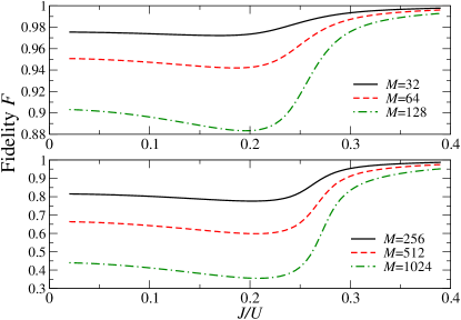
Figure 1: (color online) Fidelity in an open Bose-Hubbard chain for different system sizes and the parameter shift $\delta=0.02$.

In the former case, one sets $\hat{V}=-\sum_{i=1}^{M}\hat{a}_{i}^{\dagger}\hat{a}_{i+1}+{\rm h.c.}$ and easily finds the eigenstates of $\hat{H}(J/U=0)=\frac{1}{2}\sum_{i=1}^{M}\hat{n}_{i}\left(\hat{n}_{i}-1\right)$, which immediately leads to

$$\chi(J/U=0)=2\frac{N}{M}\left(\frac{N}{M}+1\right)M,$$ (4)

if the periodic boundary conditions and the integer filling factor are assumed. Thus $\chi(J/U=0)$ is extensive, i.e., it scales linearly with the system size at the fixed $N/M$.

In the latter case, a non-trivial result is obtained. We refer the reader to Appendix A for the details of its derivation and quote here only the final expression:

$$\chi(U/J=0)=\frac{N(N-1)}{5760M^{2}}\left(M^{4}+10M^{2}-11\right),$$ (5)

valid for periodic boundary conditions and arbitrary filling factor $N/M$. This result is super-extensive. The scaling $\chi(U/J=0)\sim M^{4}$ appears because the low-energy spectrum of a non-interacting bosonic gas in a lattice is quadratic in quasimomentum. Noting that the crossover from the quadratic to linear spectrum happens at Sto

$$\frac{U}{J}\sim\sin^{2}(k/2),$$

the qualitative departures from Eq. (5) are expected to happen at $U/J\sim\pi^{2}/M^{2}$.

For $J/U\neq 0,\infty$, Eq. (3) cannot be efficiently used to compute fidelity, and so its usefulness for the analytical characterization of fidelity of the Bose-Hubbard model is very limited.

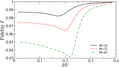
Figure 2: (color online) Fidelity in a periodic Bose-Hubbard model for different system sizes and $\delta=0.02$.

The next approach in line that seems to be simple enough to provide some analytical insights about fidelity of the Bose-Hubbard model is the Bogolubov approach Sto . There are, however, two problems associated with it. First, it does not describe physics of the Mott insulator phase possessing a finite excitation gap. Second, its validity even in the superfluid phase is questionable in 1D lattices due to the sizable population of the non-condensed atoms Sto . Since we are interested in the BKT transition of the Bose-Hubbard model, our studies are restricted to the 1D model.

Finally, the more advanced treatment of the superfluid phase is provided by the Luttinger liquid theory; see e.g. Ref. Mon (b) for the brief discussion of this theory in the Bose-Hubbard context. Luttinger liquid theory can be regarded as an effective low energy theory of systems, whose spectrum is linear in momentum and whose correlations decay algebraically Giamarchi (2006); Caz . The computation of fidelity in the Luttinger liquid theory was presented in Refs. LLf (a, b, c). While Refs. LLf (a, b) provide a definite expression for fidelity, Ref. LLf (c) argues that the zero temperature result depends on an arbitrary cut-off. This prediction is verified by comparing the Luttinger liquid theory prediction for fidelity susceptibility to the actual result in the XXZ spin chain LLf (c). Similarly as the Bose-Hubbard model, the XXZ model also undergoes a BKT transition. Therefore, we assume that the findings of Ref. LLf (c) are relevant for the Bose-Hubbard model as well.

Given all these complications, we focus on the numerics. We use Matrix Product State (MPS) techniques for both periodic ($\hat{a}_{M+1}\equiv\hat{a}_{1}$) and open ($\hat{a}_{M+1}\equiv 0$) boundary conditions. Boundary conditions significantly affect the complexity of the numerical computations.

For open boundary conditions the usual DMRG algorithm can be used White (1993, 1992); DMR . This algorithm can be naturally formulated in the MPS language Schollwöck (2011). It has allowed us to find the ground states of the Bose-Hubbard model for lattices containing up to 2048 sites at the unit filling factor. We have limited the bond dimension of the tensors forming the MPS representation to the 200 largest singular values . This has allowed us to obtain converged results for fidelity.

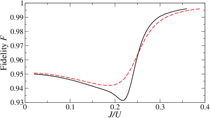
Figure 3: (color online) Black solid line shows fidelity in a periodic chain, while the dashed red line shows fidelity in an open chain. In both cases $M=64$ and $\delta=0.02$.

To find the ground state for the periodic boundary conditions, we have used imaginary time evolution technique Kub . The time evolution has been performed with the TEBD algorithm Wall and Carr (2009). In periodic chains the singular values decrease more slowly than in the open ones Verstraete et al. (2004); Pippan et al. (2010). To obtain the converged fidelity, the bond dimension 220 of the MPS vectors was necessary even for relatively small periodic systems consisting of 64 lattice sites with unit filling. In both cases the local Hilbert space has been cut to the subspace allowing at most 6 particles per site. The accuracy of our computations is discussed in Appendix B.

Finally, we mention that for $M=12$ and both open and periodic chains we have computed fidelity via exact diagonalization and compared such results to the DMRG numerics. The two approaches agree with each other.

Previous studies of fidelity of the Bose-Hubbard model at unit filling factor were restricted to $M\leq 12$ on periodic lattices (exact diagonalization) Buo and $M\leq 120$ on the open lattices (DMRG) Rig . Ref. Buo reports results on both fidelity and fidelity susceptibility, while Ref. Rig focuses on fidelity susceptibility.

III Fidelity

From now on, we set $N=M$, i.e., we study the unit filling case. Typical results that we obtain in open and periodic systems are presented in Figs. 1 and 2, respectively.

First, we notice that the minimum of fidelity lies on the Mott insulator side. This is an expected feature because the ground states near the critical point change more rapidly on the Mott insulator side of the transition (see e.g. the exponential dependence of the correlation length in the Mott phase near the critical point).

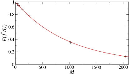
Figure 4: (color online) The minimum of fidelity as a function of the system size (open boundary conditions). Pluses come from numerics done for $\delta=0.02$ and $M=32,64,128,256,512,1024,2048$. The line represents Eq. (6) with $\alpha\simeq 2.51$ obtained from the fit.

Second, there are easy-to-notice differences between the periodic and open chain results. As shown in Fig. 3, the minimum in the open chain is much more shallow and more distant from the critical point than the one in the periodic chain. As expected, periodic chains probe quantum criticality more robustly. However, the magnitude of the difference between the two cases is surprising. It prompts separate numerical studies of the periodic and open chains.

IV Open boundary conditions

We start the discussion from looking at the value of fidelity at the minimum. We denote the position of the minimum as $J^{*}/U$. Our numerics supports the following expression

$$F(J^{*}/U,\delta)=\exp\left(-\alpha M\delta^{2}\right),$$ (6)

where $\alpha$ is some constant. Note that since we work with $N/M=1$, it is impossible to decide whether there should be $M$ or $N$ in Eq. (6).

The numerical evidence supporting Eq. (6) is discussed in detail in Figs. 4 and 5. It is worth to stress that Eq. (6) works in these figures also when $F(J^{*}/U,\delta)\ll 1$, i.e., when fidelity susceptibility fails to account for fidelity.

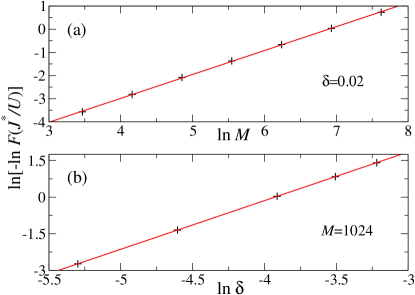
Figure 5: (color online) Scaling of the minimum of fidelity with the system size $M$ and the parameter shift $\delta$ (open boundary conditions). Panel (a): Pluses come from numerics done for $M=32,64,128,256,512,1024,2048$ rem . The line represents the fit: $\ln\left[-\ln F\left(J^{*}/U\right)\right]=-7.142+1.032\ln M$. Panel (b): Pluses come from numerics done for $\delta=0.005,0.01,0.02,0.03,0.04$ rem , while the line represents the fit: $\ln\left[-\ln F\left(J^{*}/U\right)\right]=7.833+1.994\ln\delta$. Both fits accurately support the key features of Eq. (6): $\ln F\left(J^{*}/U\right)\sim-M$ tested in panel (a) and $\ln F\left(J^{*}/U\right)\sim-\delta^{2}$ tested in panel (b).

The natural question arising now is the following: Can we extrapolate the position of the critical point by studying the scaling of $J^{*}/U$ with the system size $M$?

We were unable to find an extrapolation scheme that would give us the correct location of the critical point. We will mention below two attempts.

First, we have tested

$$\frac{J^{*}(M)}{U}=\frac{J^{*}(\infty)}{U}-\frac{a}{M^{b}},$$ (7)

with fitted parameters $J^{*}(\infty)/U=0.2114\pm 0.0003$, $a=0.53\pm 0.02$, and $b=0.73\pm 0.02$ obtained via standard Mathematica fitting procedure (Fig. 6). Thus the extrapolated position of the minimum in the infinite system, $J^{*}(\infty)/U\simeq 0.2114$, is nowhere near the expected location of the critical point $(J/U)_{c}$. The fit (7) was proposed in Ref. Buo studying fidelity of the Bose-Hubbard model, but no theory supporting it was discussed there. This fit was also used to extrapolate the position of the maximum of fidelity susceptibility in the 2D Ising model in a transverse field Albuquerque et al. (2010). The fit provided the correct location of the critical point and the critical exponent $\nu$ (following Ref. Par , it was verified in Ref. Albuquerque et al. (2010) that $b=1/\nu$ in the 2D Ising model in a transverse field; in a 1D Ising model in a transverse field $b=2/\nu$, which was shown in Refs. Par ; BDf (c)). In the Bose-Hubbard model, however, the critical exponent $\nu$ is undefined and it is unclear to us how to improve the fit (7) to properly extrapolate the position of the critical point.

Second, we tried

$$\frac{J^{*}(M)}{U}=\frac{J^{*}(\infty)}{U}-a\frac{\ln M}{M^{b}}$$ (8)

to include logarithmic finite-size corrections near the BKT transition (Fig. 6). The fit has provided $J^{*}(\infty)/U=0.2106\pm 0.0001$, $a=0.375\pm 0.007$, and $b=0.991\pm 0.006$. While this value for $J^{*}(\infty)/U$ is very close to that obtained previously, the quality of this fit is better (the inset of Fig. 6). This suggests that the finite-size correction to the position of the minimum of fidelity scales as $\ln M/M$. To quantify the difference between the fits, we provide chi-squared, i.e., the sum of the squared differences between the fitted curve and the numerical data. It equals about $2.7\times 10^{-7}$ for the fit (7) and $3.9\times 10^{-8}$ for the fit (8). Thus, the fit (8) is indeed better than the (7) one.

Finally, we look closer at fidelity per site, i.e., $\ln F/M$, which is plotted in Fig. 7. As discussed in Sec. I, this quantity is expected to have a finite non-zero value in the thermodynamic limit in the systems, where the correlation length diverges algebraically. This was predicted and observed in several models Zho ; BDf (a); Sen ; Ada . It is unclear from Fig. 7 whether the same holds for the Bose-Hubbard model. Further studies focusing on larger systems are needed to settle the system-size dependence of fidelity per site.

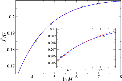
Figure 6: (color online) Position of the minimum of fidelity as a function of the system size (open boundary conditions). X’s show numerics done for $M=32,64,128,256,512,1024,2048$ and $\delta=0.02$ rem . The red (dashed) line is the fit (7) while the blue (solid) corresponds to (8). The inset shows the zoom for large $M$ to enable comparison of both fits.

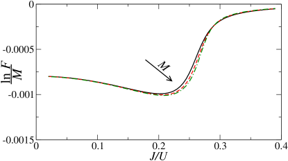
Figure 7: (color online) Fidelity per site for $\delta=0.02$ and three system sizes: $M=256,512,1024$ (black solid, red dashed, green dot-dashed, respectively). This plot is made from data from the lower panel of Fig. 1.

Next, we turn our attention to the fidelity susceptibility $\chi(J/U)$. Since fidelity (1) is symmetric with respect to the $\delta\to-\delta$ transformation, we compute

$$2\frac{1-F(J/U,\delta)}{\delta^{2}}$$

for $\delta=0.005,0.01$ and all $J/U$’s of interest and fit it with

$$\chi(J/U)+\psi(J/U)\delta^{2},$$ (9)

where $\chi(J/U)$ and $\psi(J/U)$ are the fitting parameters. We plot such obtained fidelity susceptibility in Fig. 8.

The deep Mott insulator regime, $J/U\to 0$, can be computed exactly. For open boundary conditions we get $\chi(0)=4(M-1)$ at the unit filling factor.

Similarly as in Ref. Rig , we observe that the $\chi/M$ curves cross near the critical point, i.e., around $J/U\simeq 0.287$ (the inset of Fig. 8). Indeed, we estimate from Fig. 2 of Ref. Rig that the crossing occurs there at $J/U\simeq 1/3.5\simeq 0.286$, which is completely consistent with our result. One could speculate that the position of the critical point might be linked to such a crossing, i.e., to the point where $\chi\sim M$. One should be careful, however, as such a crossing is absent in periodic systems discussed in Sec. V.

We have also studied the position of the maximum of fidelity susceptibility. For example, setting $\delta=0.02$ as in Fig. 6, we have found that the minima of fidelity and maxima of fidelity susceptibility roughly coincide (as expected, the larger the system size is, the bigger the discrepancy is). We have fitted the position of the maximum of fidelity susceptibility for $M=32,64,128,256,512,1024,2048$ with the power-law (7) and again obtained $J^{*}(\infty)/U=0.2121\pm 0.0002$.

V Periodic boundary conditions

This section presents our results on fidelity in the periodic Bose-Hubbard model. Due to the numerical limitations, the system sizes studied here are restricted to $M\leq 64$, which is the factor of $2^{5}$ smaller than the range of the system sizes considered in Sec. IV, but the factor of $2^{2}$ larger than the system sizes considered in Ref. Buo .

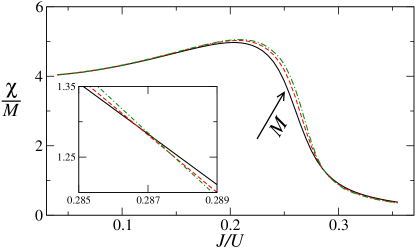
Figure 8: (color online) Fidelity susceptibility per site (open boundary conditions). The black solid, red dashed, green dot-dashed lines represent data for $M=256,512,1024$, respectively. The inset enlarges the part of the main plot, where the curves cross.

As in Sec. IV, we find numerical evidence towards the proposed scaling of the position of the minimum of fidelity (6). This is presented in detail in Fig. 9. There is no significant difference here between the open and periodic results, compare Figs. 5 and 9.

On the other hand, the extrapolation of the position of the minimum of fidelity through Eq. (7) provides a markedly different result with respect to what we have found in Sec. IV. This extrapolation is discussed in Fig. 10. The extrapolated position of the minimum in an infinite system is $J^{*}(\infty)/U=0.270\pm 0.008$, which agrees with some of the previous estimations of the position of the critical point Rig . We see also from the fit that the convergence with the system size to the asymptotic result is slow: $b=0.44\pm 0.05$ in formula (7).

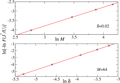
Figure 9: (color online) Scaling of the minimum of fidelity with the system size $M$ and the parameter shift $\delta$ in a periodic Bose-Hubbard chain. Upper panel: X’s show numerics for $M=16,32,48,64$ rem . The line represents the fit $\ln\left[-\ln F\left(J^{*}/U\right)\right]=-6.787+0.998\ln M$. Lower panel: X’s show numerics for $\delta=0.005,0.01,0.02,0.03,0.04$. The line represents the fit $\ln\left[-\ln F\left(J^{*}/U\right)\right]=5.104+1.982\ln\delta$.

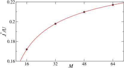
Figure 10: (color online) Position of the minimum of fidelity as a function of the system size $M$ in the periodic Bose-Hubbard model. Stars show numerics done for $\delta=0.02$ rem , while the line represents Eq. (7) with $J^{*}(\infty)/U\simeq 0.27$, $a\simeq 0.33$, and $b\simeq 0.44$ (all coming from the fit).

Next, we focus on fidelity susceptibility $\chi(J/U)$, which is plotted in Fig. 11. First, we notice again that $\chi/M\to 4$ as $J/U\to 0$. This follows from Eq. (4) taken at $N/M=1$. Moreover, it is also seen that $\chi/M$ is about the same at the maximum for all three curves ($M=16,32,64$). Second, we see from Fig. 11 that the fidelity susceptibility curves do not cross near the critical point in the periodic chain. However, they do cross near the critical point in the open chain (the inset of Fig. 8). This suggests that the inhomogeneities appearing near the edges in the open chain are responsible for the crossing in the open system (see also Sec. VI). If this is indeed the case, it is even more puzzling why the crossing occurs near the critical point in Fig. 8.

Third, we have extrapolated the position of the maximum of fidelity susceptibility with Eq. (7). Using data for $M=16,32,48,64$, we have obtained from the fit (7) that $J^{*}(\infty)/U=0.289\pm 0.008$, which again agrees with some earlier studies of the position of the critical point Rig .

Finally, at the risk of stating the obvious, we mention that it is desirable to extend these computations to larger (more critical) systems.

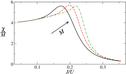
Figure 11: (color online) Fidelity susceptibility per site (periodic boundary conditions). The black solid, red dashed, green dot-dashed lines represent data for $M=16,32,64$, respectively. Fidelity susceptibility is obtained through the extrapolation procedure discussed around Eq. (9).

VI Discussion

Our results show that there is a significant difference between fidelity in the open and periodic chains. The ground states obtained in the two cases mainly differ by the occupation of the lattice sites, which is translationally invariant in a periodic chain and inhomogeneous near the edges in the open problem (Fig. 12). We believe that this inhomogeneity makes the difference, but do not have the explanation of why it is so large.

It is worth to realize that such an inhomogeneity did not cause much trouble in the determination of the location of the critical point through the studies of the decay of the correlation functions Mon (b). The ground states in these studies were obtained through the open-chain DMRG simulations, so they were the same as in our calculations. As expected, the influence of inhomogeneities on the system properties near the center was marginal for large-enough systems. Thus, one could obtain reliable results by computing the two-point correlation functions near the center.

This approach differs from the fidelity approach in one important aspect. Namely, the parts of the system near the center and those near the edges equally contribute to fidelity. We see no straightforward way to factor out the influence of the edges on fidelity. This complication follows from the simplicity of the fidelity approach, which democratically collapses all information about two ground state wave-functions into a single number.

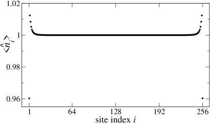
Figure 12: Density of atoms $\langle\hat{n}_{i}\rangle$ in the ground state of the open chain Bose-Hubbard model computed for $M=256$ and $J/U=0.21$, i.e., near the minimum of fidelity (Fig. 1).

We would like to stress that better understanding of our numerical results should come from the analytical derivation of the finite system-size scaling of the position of the minimum of fidelity (maximum of fidelity susceptibility) in a BKT transition. The derivation of the robust system-size-dependent scaling expressions for a BKT transition is notoriously difficult. This is seen, e.g., from the spread of the estimates of the location of the critical point. Interestingly enough, our numerics shows that the scaling law capturing the behavior of fidelity should distinguish between the open and periodic boundary conditions. Finally, we mention that our numerically-supported scaling law for fidelity at its minimum, Eq. (6), also awaits analytical explanation.

Summarizing, the key findings of this manuscript are the following. First, we have proposed and numerically verified an expression relating fidelity at the minimum, the system size, and the parameter shift (6). Second, we have found and numerically characterized the striking difference between fidelity in the open and periodic chains. Third, an exact analytical expression for fidelity susceptibility in the deep superfluid limit has been derived. We expect that these results should motivate further studies of fidelity in the Bose-Hubbard model ultimately leading to the complete understanding of the BKT transition in this model.

ACKNOWLEDGMENTS

We thank Dominique Delande for his comments about the the manuscript and suggesting logarithmic correction formula Eq. (8). BD and JZ acknowledge support of the Polish National Science Center grant DEC-2012/04/A/ST2/00088. MŁ acknowledges support the Polish National Science Center project no. 2013/08/T/ST2/00112 for the PhD thesis, special stipend of Smoluchowski Scientific Consortium “Matter Energy Future” and support by Jagiellonian University International Ph.D Studies in Physics of Complex Systems (Agreement No. MPD/2009/6 with Foundation for Polish Science). Simulations were performed at ACK Cyfronet AGH under the PL-Grid project and at IF UJ using the Deszno supercomputer purchased in the framework of the Polish Innovation Economy Operational Program (POIG.02.01.00-12-023/08).

Appendix A Fidelity susceptibility at $U/J=0$

We will use Eq. (3) to compute fidelity susceptibility at $\lambda=U/J=0$. Thus,

$$\hat{H}(U/J=0)=-\sum_{i=1}^{M}\hat{a}_{i}^{\dagger}\hat{a}_{i+1}+{\rm h.c.},$$ (10)

where $\hat{a}_{M+1}\equiv\hat{a}_{1}$ and

$$\hat{V}=\frac{1}{2}\sum_{i=1}^{M}\hat{n}_{i}\left(\hat{n}_{i}-1\right).$$

The eigenstates of the Hamiltonian (10) can be obtained in a standard way Sto . By going to the momentum space

$$\hat{a}_{j}=\frac{\sum_{k}\exp(ikj)\hat{b}_{k}}{\sqrt{M}},\ k=0,\frac{2\pi}{M},\frac{4\pi}{M},\dots,2\left(\pi-\frac{\pi}{M}\right),$$

one finds that

$$\hat{H}(U/J=0)=-2\sum_{k}\cos(k)\hat{b}^{\dagger}_{k}\hat{b}_{k}.$$

All particles occupy the zero momentum mode in the ground state: $|\phi_{0}(U/J=0)\rangle=|N,0,\dots\rangle$. The perturbation operator has to be transformed to the momentum space as well, and its action on the ground state is the following

$$\hat{V} |\phi_{0}(U/J=0)\rangle=\frac{N(N-1)}{2M}|\phi_{0}(U/J=0)\rangle$$

$$+ \frac{\sqrt{N(N-1)}}{2M}\sum_{k\neq 0}\hat{b}^{\dagger}_{2\pi-k}\hat{b}^{\dagger}_{k}|N-2,0,\dots\rangle.$$

One can now use Eq. (3) to obtain

$$\chi(U/J=0) =\frac{N(N-1)}{64M^{2}}\left(\sum_{k^{\prime}}\frac{1}{\sin^{4}(k^{\prime})}+\frac{1}{2}\right),$$ (11)

$$k^{\prime} =\frac{\pi}{M},\frac{2\pi}{M},\dots,\frac{\pi}{M}\frac{M-2}{2},$$

for even $M$ and

$$\chi(U/J=0) =\frac{N(N-1)}{64M^{2}}\sum_{k^{\prime\prime}}\frac{1}{\sin^{4}(k^{\prime\prime})},$$ (12)

$$k^{\prime\prime} =\frac{\pi}{M},\frac{2\pi}{M},\dots,\frac{\pi}{M}\frac{M-1}{2},$$

for odd M. The sums over $k^{\prime}$ and $k^{\prime\prime}$ can be evaluated with the technique proposed in Ref. BDf (c).

The evaluation of the sum (11) proceeds from the identity Ryz

$$\sum_{k^{\prime}}\left[\frac{\sin^{2}(k^{\prime})}{\sinh(x)}+\frac{\tanh(x/2)}{2}\right]^{-1}=f(x),$$ (13)

$$f(x)=M\coth\left(\frac{Mx}{2}\right)-2\coth(x).$$

Dividing this expression by $\sinh(x)$ and then taking its derivative with respect to $x$ we get

$$\sum_{k^{\prime}}\left[\sin^{2}(k^{\prime})+\sinh^{2}(x/2)\right]^{-2}=-\frac{2}{\sinh(x)}\frac{d}{dx}\left(\frac{f(x)}{\sinh(x)}\right).$$ (14)

The limit of $x\to 0$ of Eq. (14) provides

$$\sum_{k^{\prime}}\frac{1}{\sin^{4}(k^{\prime})}=\frac{M^{4}+10M^{2}-56}{90}.$$ (15)

One can compute the sum in Eq. (12) by replacing $k^{\prime}$ by $k^{\prime\prime}$ and $f(x)$ by $M\coth(Mx/2)-\coth(x/2)$ in Eq. (13), and then repeating the steps leading to Eqs. (14) and (15). In the end, we get

$$\sum_{k^{\prime\prime}}\frac{1}{\sin^{4}(k^{\prime\prime})}=\frac{M^{4}+10M^{2}-11}{90}.$$ (16)

Combining Eqs. (11) and (15) and also Eqs. (12) and (16), one obtains

$$\chi(U/J=0)=\frac{N(N-1)}{5760M^{2}}\left(M^{4}+10M^{2}-11\right),$$

for any system size $M>1$ and the number of atoms $N>1$.

Appendix B Convergence of numerical simulations

The accuracy of our numerical computation of fidelity is mainly affected by the accuracy of the determination of the ground states of the Bose-Hubbard Hamiltonian. For the later, we use the DMRG and TEBD algorithms for the open and periodic systems, respectively. Both numerical approaches express the ground state through the MPS ansatz.

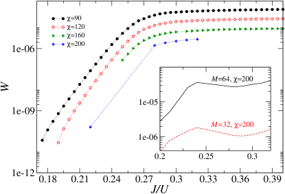
Figure 13: (color online) Total discarded weights for the computation of ground states. The main plot shows data for the open Bose-Hubbard chain of length $M=512$. The inset shows the same for the periodic system.

The errors in the DMRG calculations appear mainly during the so-called local updates, where the predetermined number of the eigenvectors of the reduced density matrix with largest eigenvalues $\lambda_{i}^{2}$ is kept. We keep up to $\chi=200$ eigenvectors out of the superblock dimension $d\chi=1400$ ($d$ is the on-site Hilbert space dimension; $\chi$ in this section should not be confused with fidelity susceptibility). Let $k$ denote the site at which the local update is considered. The weight of the discarded eigenvectors is

$$W_{k}=\sum\limits_{i=\chi+1}^{d\chi}\lambda_{i}^{2}$$

for that local update. Fig. 13 shows the total discarded weights $W=\sum_{k}W_{k}$ as a function of the ratio $J/U$ and the bond dimension $\chi$.

It shows that total discarded weights are certainly negligible around $J/U=0.21$, where we study the minima of fidelity (Figs. 4–6). In particular, we find that for all studied system sizes, $M=32,\dots,2048$, $F(J/U=0.21,\delta=0.02)$ obtained for $\chi=180$ and $\chi=240$ differ by less than $0.001\%$.

On the other hand, for large $J/U$, say $J/U>0.3$ for which the infinite system is superfluid, the discarded weights are non-negligible. As a result, we find that $1-F(J/U=0.3,\delta=0.02)$ for $\chi=160$ and $\chi=200$ differ by about $2\%$ for the system size $M=512$ (we compare here $1-F$ instead of $F$ because fidelity approaches unity in this regime of parameters). This accuracy is sufficient for our qualitative discussion of fidelity in the superfluid limit. Finally, we mention that in the DMRG calculations the sweeps across the system have been performed until the energy of the ground state reached a stationary value.

The ground state in the periodic system was obtained by the imaginary time evolution using the TEBD algorithm Wall and Carr (2009). Similarly as in the DMRG calculation, the maximal discarded weights can be computed. We plot them in the inset of Fig. 13. Since the eigenvalues $\lambda^{2}_{i}$ decrease much slower than in the periodic case, we have to focus on small systems. This quick loss of accuracy with the system size can be illustrated by computing fidelity for $M=32$ and $M=64$. We find that $F(J/U=0.21,\delta=0.02)$ differs for $\chi=180$ and $\chi=240$ by about $0.001\%$ when $M=32$. For $M=64$, however, this difference grows to almost $4\%$. Thus, our results for fidelity in the periodic case are accurate near the minimum to a few percent for $M=64$ and to a fraction of a percent for smaller system sizes. This is sufficient for our quantitative study of the location of the minimum of fidelity.

Finally, we would like to mention that the computation of a single ground state in an open (periodic) chain of length 2048 (64) on a single core 2.6 GHz Intel Xeon processor takes us over a month. Thus, the extension of these studies to larger systems will require the engagement of massive computer resources.

References

- Zanardi and Paunković (2006) P. Zanardi and N. Paunković, Phys. Rev. E 74, 031123 (2006).
- Sachdev (2011) S. Sachdev, Quantum Phase Transitions (Cambridge University Press, Cambridge, U.K., 2011).
- Continentino (2001) M. A. Continentino, Quantum Scaling in Many-Body Systems (World Scientific Publishing, Singapore, 2001).
- (4) S. Sachdev, Phys. Today 64, 29 (2011).
- (5) S.-J. Gu, Int. J. Mod. Phys. B 24, 4371 (2010).
- Albuquerque et al. (2010) A. F. Albuquerque, F. Alet, C. Sire, and S. Capponi, Phys. Rev. B 81, 064418 (2010).
- (7) V. Gritsev and A. Polkovnikov, in Understanding in Quantum Phase Transitions edited by L. Carr (Taylor & Francis, Boca Raton, 2010); arXiv:0910.3692.
- BDf (a) M. M. Rams and B. Damski, Phys. Rev. Lett. 106, 055701 (2011).
- (9) H.-Q. Zhou, J.-H. Zhao, and B. Li, J. Phys. A 41, 492002 (2008).
- BDf (b) M. M. Rams and B. Damski, Phys. Rev. A 84, 032324 (2011).
- (11) H. A. Gersch and G. C. Knollman, Phys. Rev. 129, 959 (1963).
- Fisher et al. (1989) M. P. Fisher, P. B. Weichman, G. Grinstein, and D. S. Fisher, Phys. Rev. B 40, 546 (1989).
- (13) D. Jaksch et al., Phys. Rev. Lett. 81, 3108 (1998).
- (14) M. Greiner, O. Mandel, T. Esslinger, T. W. Hänsch, and I. Bloch, Nature (London) 415, 39 (2002).
- Stöferle et al. (2004) T. Stöferle, H. Moritz, C. Schori, M. Köhl, and T. Esslinger, Phys. Rev. Lett. 92, 130403 (2004).
- Lewenstein et al. (2012) M. Lewenstein, A. Sanpera, and V. Ahufinger, Ultracold Atoms in Optical Lattices: Simulating quantum many-body systems (Oxford University Press, 2012).
- (17) R. V. Pai, R. Pandit, H. R. Krishnamurthy, and S. Ramasesha, Phys. Rev. Lett. 76, 2937 (1996).
- Mon (a) T. D. Kühner and H. Monien, Phys. Rev. B 58, R14741 (1998).
- (19) P. Buonsante and A. Vezzani, Phys. Rev. Lett. 98, 110601 (2007).
- (20) J. Carrasquilla, S. R. Manmana, and M. Rigol, Phys. Rev. A 87, 043606 (2013).
- (21) In virtually all experiments the harmonic trapping potential is present adding the local density-dependent term to the Hamiltonian. From the theoretical point of view, the properties of a homogeneous system are more interesting and we shall consider such a system. Recent progress in experimental techniques shows that homogeneous models can be experimentally realized Gaunt et al. (2013).
- Essler et al. (2005) F. H. L. Essler, H. Frahm, F. Göhmann, A. Klümper, and V. E. Korepin, The One-Dimensional Hubbard Model (Cambridge University Press, Cambridge, UK, 2005).
- (23) D. van Oosten, P. van der Straten, and H. T. C. Stoof, Phys. Rev. A 63, 053601 (2001).
- Mon (b) T. D. Kühner, S. R. White, and H. Monien, Phys. Rev. B 61, 12474 (2000).
- Giamarchi (2006) T. Giamarchi, Quantum Physics in One Dimension (Clarendon Press, Oxford, U.K., 2006).
- (26) M. A. Cazalilla, J. Phys. B 37, S1 (2004).
- LLf (a) M.-F. Yang, Phys. Rev. B 76, 180403(R) (2007).
- LLf (b) J. O. Fjærestad, J. Stat. Mech.: Theory Exp. P07011 (2008).
- LLf (c) J. Sirker, Phys. Rev. Lett. 105, 117203 (2010).
- White (1993) S. R. White, Phys. Rev. B 48, 10345 (1993).
- White (1992) S. R. White, Phys. Rev. Lett. 69, 2863 (1992).
- (32) G. De Chiara, M. Rizzi, D. Rossini, S. Montangero, J. Comput. Theor. Nanosci. 5, 1277 (2008).
- Schollwöck (2011) U. Schollwöck, Annals of Physics 326, 96 (2011).
- (34) J. Zakrzewski and D. Delande, in Proceedings of Let’s Face Chaos Through Nonlinear Dynamics, 7th Interna- tional Summer School and Conference (AIP, 2008), Vol. 1076, pp. 292-300 (2008).
- Wall and Carr (2009) M. L. Wall and L. D. Carr, Open Source TEBD (2009).
- Verstraete et al. (2004) F. Verstraete, D. Porras, and J. I. Cirac, Phys. Rev. Lett. 93, 227205 (2004).
- Pippan et al. (2010) P. Pippan, S. R. White, and H. G. Evertz, Phys. Rev. B 81, 081103 (2010).
- (38) We compute fidelity on the discrete grid and use the standard cubic spline technique to locate its minimum, i.e., . Thus, the upper bound on the error bar of is . A more careful estimate of the error bar of each point in Figs. 6 and 10 can be obtained as follows. First, for every system size that we study, we recalculate fidelity on the grid, which is twice larger then the original one that we employ. Then, we again use the cubic spline technique to compute the position of the minimum of fidelity. We find that for all system sizes computed for and differ by less than . This suggests that the error bars on the data points that we use for the fit are negligible.
- (39) P. Zanardi, M. G. A. Paris, and L. Campos Venuti, Phys. Rev. A 78, 042105 (2008).
- BDf (c) B. Damski, Phys. Rev. E 87, 052131 (2013).
- (41) V. Mukherjee, A. Dutta, and D. Sen, Phys. Rev. B 85, 024301 (2012).
- (42) M. Adamski, J. Jȩdrzejewski, and T. Krokhmalskii, J. Stat. Mech. P07001 (2013).
- (43) I. S. Gradshteyn and I. M. Ryzhik, Table of Integrals, Series, and Products, 7th ed. (Academic Press, San Diego, 2007).
- Gaunt et al. (2013) A. L. Gaunt, T. F. Schmidutz, I. Gotlibovych, R. P. Smith, and Z. Hadzibabic, Phys. Rev. Lett. 110, 200406 (2013).