Chaotic Interference and Quantum-Classical Correspondence: Mechanisms of Decoherence and State Mixing

I Outline

The famous Nils Bohr’s quantum-classical correspondence principle states that the classical mechanics is a limiting case of the more general quantum mechanics. This implies that ‘‘under certain conditions" quantum laws of motion become equivalent to classical ones. One of the conditions is fairly obvious: the corresponding classical action should be very large as compared with the Planck’s constant $\hbar$. But is this the sufficient condition? In fact, it is not!

The quantum laws show up in two different, although not entirely independent ways:

1. discrete spectrum of finite motion,

2. interference phenomena.

Even if the energy spectrum of a finite closed quantum system becomes continuous in the formal limit of vanishing $\hbar$, the interference effects cannot disappear in similar manner. Indeed, a quantum wave functions has no definite classical counterpart. Meanwhile, suppression of effects of quantum interference ("decoherence") is a key requirement for the classical laws to appear. Being, in essence, of quite general nature, this problem takes on special significance in the non-trivial case of non-linear classically chaotic quantum systems.

A number of typical manifestations of the quantum coherence in the time evolution as well as eigenstates’ properties are widely discussed in the scientific literature:

• Wave packet dynamics and decay of quantum fidelity.

• Universal local spectral fluctuations.

• Scars in the stationary eigenfunctions.

• Elastic enhancement in chaotic resonance scattering.

• Weak localization in transport phenomena.

The specific features of quantum dynamics of classically chaotic systems seem to be in striking contrast with those of genuine classical chaos. Since these features can even question the validity of the quantum-classical correspondence principle by itself, a more profound analysis is needed for understanding the bridge between the classical and quantum chaotic worlds.

I.1 Chaotic time evolution

In the case of regular classical dynamics, the system’s response to a weak external perturbation is proportional to its strength and the system may be still treated as a closed one during sufficiently long time. In contrast, chaotic classical dynamics is exponentially unstable and therefore it is extremely sensitive to any uncontrollable external influence. We can never neglect the influence of the environment. This therefore stipulates the self-mixing property of classical dynamical chaos and, as a consequence, a very fast decay of the phase correlations (here and throughout the paper we use the language of action-angle variables).

Whereas the exponential decay of the phase correlations is an underlying feature of the classical dynamical chaos Chiri79 , the so called "quantum chaos", i.e. quantum dynamics of classically chaotic systems is not by itself capable of destroying the quantum phase coherence. Strictly speaking, any initially pure quantum state remains pure during arbitrary long evolution. Quantization of the phase space removes exponential instability and makes the quantum dynamics to be substantially more stable than the classical one. There exists a threshold $\sigma_{c}(t)$ of the external noise strength $\sigma$ below which the coherence survives up to the time $t$ Sokol08 ; Sokol08a ; Sokol09 Only appreciably strong noise or finite measurement accuracy can produce a mixture of quantum states sufficient for noticeable suppression of quantum coherence. A number of appropriate characteristics: Peres fidelity $F(t)$, purity $\mathbb{P}(t)$, Shannon (information) ${\cal I}(t)$ and von Neumann (correlational) ${\cal S}(t)$ entropies are used to demonstrate the gradual loss of quantum coherence during system’s evolution in the presence of noisy background. Being sensitive to the quantum coherence, the von Neumann entropy remains smaller than the Shannon entropy but runs up monotonically to the latter when the evolution time approaches some moment $t_{(dec)}$ when decoherence becomes complete. After this time, the system occupies the whole phase space volume accessible at the running degree of excitation energy thus reaching a sort of equilibrium. Henceforth the phase volume expands ‘‘adiabatically’’: the both entropies remain almost constant. The evolution after the time $t_{(dec)}$ is Markovian Sokol09 .

I.2 2D billiards

The plain ($2D$) areas with closed irregular borders called billiards are pet systems often used to illustrate characteristic features of the classical dynamical chaos. With the advent of the ability to fabricate mesoscopic analogs of the classical billiards the opportunity appeared to observe experimentally the signatures of chaos in classically chaotic quantum systems. An excellent possibility thus has arisen to verify the theoretical concepts developed in numerous theoretical investigations of "quantum chaos" phenomena. Extensive study of the electron transport through ballistic $2D$ meso-structures Jalab90 ; Marcu92 (see also Beena97 ; Alhas00 and references therein) have fully confirmed correctness of the basic ideas Izrai90 ; Gutzw90 ; Haake91 of the theory of the chaotic quantum interference and relevance Baran94 ; Beena97 ; Alhas00 of the so called random-matrix approach Verba85 ; Mello85 ; Mehta91 to the problem of the universal spectral fluctuations as well as conductance fluctuations in open mesoscopic set-ups (see sec.I.5).

The energy $E$ is the only integral of motion in a closed billiard. Repeating reflections from the border produces a countless manifold of unclosed exponentially unstable trajectories and, as a consequence, chaotic dynamics. At the same time, there exists a countable set of specific, but also exponentially unstable, periodic orbits. The number $N(T)$ of the latter trajectories grows exponentially with the period $T$ as $N(T)\sim e^{\frac{T}{\tau_{c}}}$ with the characteristic time $\tau_{c}$ directly connected, $\tau_{c}\thicksim 1/\Lambda$, to the Lyapunov exponent $\Lambda$ that describes the exponential instability Zasla85 . Meanwhile, in contravention with the classical exponential instability, stable interference maxima (scars) along the periodic classical orbits (alongside with irregularly scattered point-like interference maxima (specks)) are discovered numerically Helle84 in the stationary billiard’s eigenstates even in the very deep semi-classical region . Does this fact compromises the quantum-classical correspondence principle?

To answer afore-posed question let us consider first an elementary example of $1D$ finite motion. A particle with a mass $m$ and energy $E$ moves in a potential well. The classical position probability density is proportional to the fraction of the period of oscillations the particle spends near a point $x$ and is easily found to be:

$$w_{c}(x)=\left\{\begin{array}[]{ll}0&x\notin[a,b],\\ \frac{m\,\omega_{c}(E)}{\pi\,p_{c}(x)},&x\in[a,b]\,.\\ \end{array}\right.$$ (1)

where $p_{c}(x)=\sqrt{2m\left[E-U(x)\right]}$ is the particle’s classical momentum at the point $x$ and $\omega_{c}(E)$ is the frequency of classical oscillations between the turning points $a$ and $b$.

On the other hand the semi-classical solution of the corresponding quantum problem yields

$$w_{n}(x) = |\psi_{n}(x)|^{2}$$ (4)

$$= \left\{\begin{array}[]{ll}e^{\{-\frac{2}{\hbar}\int_{x}^{a}dx^{\prime}|p_{c}(x^{\prime})|\}},e^{\{-\frac{2}{\hbar}\int_{b}^{x}dx^{\prime}|p_{c}(x^{\prime})|\}}&\rightarrow 0,\\ \frac{m\,\omega_{c}(E_{n})}{\pi\,p_{c}(x)}\,2\cos^{2}\{\frac{1}{\hbar}\int_{a}^{x}dx^{\prime}p_{c}(x^{\prime})-\frac{\pi}{4}\}&\rightarrow?\end{array}\right.$$

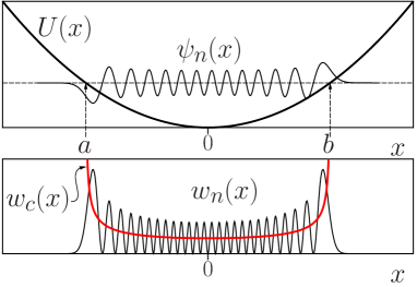
Figure 1: Top: wave function of harmonic oscillator for the energy level $n=25$; bottom: corresponding probability distributions are shown by thick red and thin black lines for classical and quantum cases respectively.

As expected (see the simplest of linear oscillator, Fig.1, bottom frame), the probability density (4) vanishes in the classically forbidden region when the semi-classical parameter goes to infinity but there exists no reasonable result in the classically allowed interval. The wildly fluctuating without approaching a certain limit cosine-square factor appears from the interference of two waves running in the opposite directions. To attain the classical result (1) an additional averaging over some finite either position $\Delta x$ or energy $\Delta n$ intervals around fixed $|x\rangle$ or $|n\rangle$ states is necessary.

$$\overline{w_{n}(x)}^{(x)} = \langle n|\left(\int_{x^{\prime}\in\Delta x}dx^{\prime}\,\mathbf{p}_{x}(x^{\prime})|x^{\prime}\rangle\langle x^{\prime}|\right)|n\rangle=\langle n|{\hat{\rho}}^{(x)}|n\rangle$$ (5)

$$\overline{w_{n}(x)}^{(n)} = \langle x|\left(\sum_{n^{\prime}\in\Delta n}\mathbf{p}_{n}(n^{\prime})|n^{\prime}\rangle\langle n^{\prime}|\right)|x\rangle=\langle x|{\hat{\rho}}^{(n)}|x\rangle\,.$$ (6)

The density matrices ${\hat{\rho}}^{(q)}$ $(q=n,x)$ describe incoherent mixtures of the quantum states within the indicated intervals. The real and normalized to unity quantities $\mathbf{p}$ characterize the weights of these states. Obviously, the range of averaging $\Delta x$ should satisfy the condition $\Delta x\geqslant\pi\hbar/p_{c}(x)$ to meet the classical behavior. Similar reasoning leads to the condition $\Delta E\approx\Delta n\,\hbar\omega_{c}\geqslant 2\pi\hbar/T$ where $T=2\int_{a}^{b}dx/v_{c}(x)$ is the period of classical oscillations. Similarly, averaging over the energy interval $\Delta E$ wipes off all scars of eigenstates of a $2D$ billiard with the periods $T>\hbar/\Delta E$, whereas those with smaller periods still survive Bogom88 .

Strictly speaking, decoherence is not perfect as long as off-diagonal matrix elements of the density matrix still exist. They are complex and their phases carry some information on the more subtle interference effects. Complete decoherence is achieved only when the number of mixing states is so large that the density matrix becomes proportional to the unit matrix and ceases to depend on the basis in the Hilbert space of states. As a matter of fact, decoherence can originate only from: (i) the process of preparation of initially mixed state, and (ii) mixing induced during the time evolution by a persisting external noise.

I.3 The basics of quantum mixed states.

The concept of mixed states plays a paramount role in the problem of decoherence. A pure quantum state is specified at some moment of time $t$ by its wave vector $|\psi(t)\rangle$ in the Hilbert space. This allows, in particular, calculation of the mean value $O(t)=\langle\psi(t)|{\hat{O}}|\psi(t)\rangle$ (in what follows we suggest this vector to be normalized to unity, $\langle\psi(t)|\psi(t)\rangle$=1) of any dynamical quantity represented by a Hermitian operator ${\hat{O}}$. Equivalently, the same state can be described by the density matrix ${\hat{\rho}(t)=|\psi(t)\rangle}\langle\psi(t)|$ that satisfies two obvious conditions:

$$Tr{\hat{\rho}}(t)=1,\quad{\hat{\rho}}^{2}(t)={\hat{\rho}}(t).$$ (7)

The second relation is the necessary and sufficient condition of purity of a quantum state. With these definitions at hands, the mean values can be presented in one of the following forms

$$O(t)=\langle\psi(t)|{\hat{O}}|\psi(t)\rangle=Tr\left[{\hat{O}}\,{\hat{\rho}}(t)\right]=\sum_{m,n}O_{nm}(t)\rho_{mn}(t).$$ (8)

The expression in the right hand side represents the same mean value in the basis of a complete set of motionless vectors $|n\rangle$ in the Hilbert space. Since the density matrix is Hermitian, all its diagonal elements $\rho_{nn}(t)$ are real.

Like any Hermitian matrix, the density matrix $\rho_{mn}(t)$ can be diagonalized with the help of some unitary transformation. On account of the conditions (7) the density matrix of a pure quantum state has only one nonzero eigenvalue that equals one. Obviously, the diagonalization returns us to the original form ${\hat{\rho}(t)=|\psi(t)\rangle}\langle\psi(t)|$. The transformation matrix depends on time if the system undergo time evolution. In practice, a fixed basis of states $|n\rangle$ is, as a rule, a more relevant choice from physical point of view.

A mixed quantum state is described at any moment of time $t$ by an incoherent sum

$${\hat{\rho}}(t)=\sum_{k}\mathbf{p}_{k}(t)|v_{k}(t)\rangle\langle v_{k}(t)|$$ (9)

of binary contributions where the states $|v_{k}(t)\rangle$ are the eigenvectors of the density matrix when $0\leq\mathbf{p}_{k}(t)\leq 1$ stand for the weights of the corresponding pure fragments. These weights do not actually depend on time during dynamical evolution described by some unitary evolution matrix ${\hat{U}}(t)$. It is not the case, however, if the system interacts with a noisy background.

In the fixed basis $|n\rangle$, an initially diagonal incoherent mixture develops off-diagonal elements even during unitary dynamical evolution. There exists, however, a convenient invariant measure of state purity called Purity

$$\mathbb{P}(t)=\mathrm{Tr}\left[{\hat{\rho}}^{2}(t)\right]=\sum_{k}\mathbf{p}^{2}_{k}=\mathbb{P}(0)$$ (10)

that remains constant as long as the noise is absent. The Purity is restricted to the interval $0\leq\mathbb{P}\leq 1$ and is mounting to one in the limit of a perfectly pure state. In many respects similar properties are inherent in the invariant von Neumann entropy

$${\cal S}(t)=-\mathrm{Tr}\left[{\hat{\rho}}(t)\ln{\hat{\rho}}(t)\right]={\cal S}(0)$$ (11)

which vanishes only in the case of a perfectly pure state.

It is very useful to transfer the story on the, generally mixed, quantum states evolution to the language of the phase space Agarw70 ; Agarw70a ; Sokol08a . This elucidates analogy and distinctions between classical and quantum dynamics. A double Fourier transformation of the density matrix

$$\begin{array}[]{c}W(\alpha^{*},\alpha;t)=\frac{1}{\pi^{2}\hbar}\int d^{2}\eta\,\exp\left(\eta\frac{\alpha^{\star}}{\sqrt{\hbar}}-\eta^{\star}\frac{\alpha}{\sqrt{\hbar}}\right)\tilde{\rho}(\eta^{\star},\eta;t)=\\ \frac{1}{\pi^{2}\hbar}\int d^{2}\eta\,\exp\left(\eta^{*}\frac{\alpha}{\sqrt{\hbar}}-\eta\frac{\alpha^{*}}{\sqrt{\hbar}}\right)\mathrm{Tr}\left[{\hat{\rho}(t)}\,{\hat{D}(\eta)}\right]\,,\end{array}$$ (12)

with the operator ${\hat{D}(\eta)}=\exp(\eta\,{\hat{a}}^{{\dagger}}-\eta^{*}{\hat{a}})$ being the coherent states displacement defines the Wigner function $W(\alpha^{*},\alpha;t)$ that is a direct quantum counterpart of the classical phase space distribution function $W^{(c)}(\alpha^{*},\alpha;t)$. The complex variables $\alpha^{*},\alpha$ are connected with the standard action-angle variables $I,\theta$ by the canonical transformations $\alpha=\sqrt{I}e^{-i\theta},\,\alpha^{*}=\sqrt{I}e^{i\theta}$.

Deep and detailed analysis of properties of the density matrix and its significant role for the problem of decoherence has been presented in the review Zurek03 .

I.4 Peres fidelity

Response of an evolving in time quantum system to a weak external perturbation is of prime interest in the context of the problem of stability and reversibility of quantum motion. The customary quantitative characteristic of sensitivity of classically chaotic quantum dynamics to such perturbations is the Peres fidelity Peres84 :

$$F(t)=\frac{\mathrm{Tr}\left[{\hat{\rho}}_{H}(t)\,{\hat{\rho}}_{H^{\prime}}(t)\right]}{\mathbb{P}(t)}=\frac{\sum_{kl}{\bf p}_{k}{\bf p}^{\prime}_{l}\big{|}\langle v_{k}(t)|v^{\prime}_{l}(t)\rangle\big{|}^{2}}{\mathbb{P}(t)}\,.$$ (13)

Fidelity measures the weighted mean distance between two, generally mixed, quantum states evolving according to slightly different Hamiltonians ${\hat{H}}$ and ${\hat{H}}^{\prime}$, is bounded in the interval $[0,1]$ and equals one when ${\hat{H}}^{\prime}={\hat{H}}$. Its time decay due to diminishing of the overlap of $v$-eigenvectors elucidates the sensitivity of the motion to an external influence. In particular, this quantity enable one to directly connect stability and reversibility of quantum dynamics with complexity of the quantum Wigner function. More than that, the notion of the Peres fidelity directly extends to the classical mechanics (see sec.II in Benen03 and Benen03a ). The number of $\theta$-harmonics can serve (see below) as a natural quantitative measure of complexity of the both, classical as well as quantum phase space (quasi-)distributions Sokol08a (see, however, Benen12 where another measure of complexity has been proposed that is relevant in the case of systems with more than one degrees of freedom).

I.5 Open mesoscopic billiards and electron quantum transport

Scattering of quantum particles by 2D billiard-like mesoscopic structures connected to the continuum by two opening leads each supporting $M$ channels is an intriguing issue that attracted a lot of attention of theorists as well as experimentalists for at least the last two decades. If the mean free path of such a particle exceeds the typical size of the structure the particle’s dynamics inside it strongly depends on the shape of its border. The classical motion in this case becomes stochastic and quantum scattering is expected to be described well within the framework of the random matrix approach to the resonance scattering theory. Intensive experimental studies confirmed in many respects these expectations. Nevertheless, electron transport experiments with ballistic quantum dots reveal noticeable and persisting up to zero temperature loss of the quantum-mechanical coherence in contravention of predictions of the random-matrix as well as semiclassical scattering theories.

There exists a number of different methods of accounting for the decoherence effect in the ballistic quantum transport processes.As a matter of fact, all of them originate from the pioneering Büttiker’s ideas Buetti86 . The dot is supposed to be connected someway with a bath of electrons so that the dot and the bath can exchange electrons in such a manner that the mean exchange electric current vanishes. Since the incoming electron carries no information of the phase of the wave function in the dot, the coherence turns our to be suppressed. The cost payed is that the number of particle is conserved only in average during the scattering so that the scattering matrix is not, strictly speaking, unitary. An alternative approach has been therefore proposed in Beena05 with a closed long stub instead of an opening lead. Thereby unitarity of the $S$-matrix is guaranteed and none of the electrons is lost at any individual act of scattering.

Decoherence takes place in this case because of a spatially random time-dependent external electric field that acts in the stub. As a result, an electron once penetrated the stub return back in the dot without whatever phase memory.

In spite of the advantages of the stub model the necessity of introducing ad hoc an external time dependent potential seems to be somewhat artificial. Still another possibility arises if a time-independent weak interaction is taken into account with a relatively rare irregular impurities in the semiconductor heterostructure to whose interface region the electrons are confined. At that, unavoidable experimental averaging over the scattering energy on account of finite experimental accuracy in measuring the cross sections is a point of primary importance.

Due to the interaction with environment, each ‘‘doorway’’ resonance state excited in the structure via external channels gets fragmented onto a large number $\sim\Gamma_{s}/d$ (the spreading width $\Gamma_{s}$ characterizes the strength of the coupling to the environment when $d$ is the single-quasi-particle mean level spacing) of very narrow resonances Sokol10 . Only the cross sections averaged over the fine $(\thicksim d)$ structure scale are observable. Due to such an averaging the doorway resonance states are damped not only because of escape through such channels but also due to the ulterior population of the relatively long-lived environmental states. As a result, transmission of an electron with a given incoming energy $E_{in}$ through the structure turns out to be an incoherent sum of the flow formed by the interfering damped doorway resonances and the retarded flow of the particles re-emitted into the structure by the environment. Being delayed, the returning electrons do not interfere with those that escape directly through the external leads.

The temporal characteristics of the transport are described in detail by the $M\times M$ Smith time delay matrix $Q=-iS^{{\dagger}}dS/dE=Q^{(s)}+Q^{(e)}$ that consists of two contributions $Q^{(s,e)}$. They correspond respectively to the (modified due to the interaction with the background) time delay within the dot and additional delay because of the temporary transitions into the background.

We suppose the temperature of the environment to be zero whereas the energy of the incoming particle $E_{in}$ can be close to or somewhat above the Fermi surface of electrons in the environment. Therefore, though the number of the particles is definitely conserved in each individual event of transmission, there exists a probability that some part of the electron’s energy can be absorbed due to environmental many-body effects. The both decoherence and absorption phenomena can be naturally treated within the framework of a unit microscopic model based on the general theory of the resonance scattering. Both these effects are controlled by the only parameter: the spreading width of the doorway resonances.

If the energy $E_{in}$ noticeably exceeds the environment’s Fermi surface and the doorway resonances overlap, the random matrix approach becomes relevant and ensemble averaging in the doorway sector is appropriate. Such an averaging, being equivalent to the energy averaging over the doorway scale $D$, suppresses all interference effects save the elastic enhancement phenomenon. The latter is a direct consequence of the time reversal symmetry and manifests itself in the so called weak localization effect. However the energy absorption in the environment violates this symmetry and suppresses the weak localization.

II Particulars

II.1 An example of chaotic classical dynamics

As an instructive and typical example of chaotic classical system we consider below a periodically kicked quartic nonlinear oscillator

$$H(\alpha^{*},\alpha;t)=H^{(0)}+H^{(k)},$$ (14)

where the unperturbed Hamiltonian function reads

$$H^{(0)}(\alpha^{*},\alpha)=\frac{p^{2}}{2m}+\frac{\omega^{2}_{0}}{4}\tan^{2}(\sqrt{2m}\,x)=\omega_{0}\,|\alpha|^{2}+|\alpha|^{4},$$ (15)

and the time-dependent perturbation

$$H^{(k)}(\alpha^{*},\alpha;t)=g(t)=g_{0}\sum_{\tau}\delta(t-\tau)\,(\alpha^{*}+\alpha).$$ (16)

constitutes a sequence of periodic kicks with strength $g_{0}$ that are acting at the instances $\tau=\pm 1,\pm 2,...\,$.

There are two convenient choices of the canonical variables in this case: $I,\theta$ or $\alpha,i\alpha^{*}$ related by the canonical transformation $\alpha=\sqrt{I}\,e^{-i\theta}$, $\alpha^{*}=\sqrt{I}\,e^{i\theta}$. The action-angle variables $I,\theta$ are ordinary used in the classical considerations. On the other hand, the advantage of $\alpha$-variables is that they are directly related to the quantum creation-annihilation operators ${\hat{a}}^{\dagger},{\hat{a}}$. The action-angle variables satisfy along a given phase trajectory two coupled nonlinear equations Sokol84 :

$$I(t) = \left|{\sqrt{{\overset{\circ}{I}}}+i\int_{0}^{t}d\tau g(\tau)e^{i[\theta(\tau)-\overset{\circ}{\theta}]}}\right|^{2}$$ (17)

$$\theta(t) = \int_{0}^{t}d\tau[\omega_{0}+2I(\tau)]$$ (18)

(here and in what follow we mark the initial values by the overset circle). A great majority of trajectories becomes exponentially unstable and, the corresponding motion is globally chaotic when the strength of the kicks exceeds 1: $|g_{0}|>1$. Under this condition the phase correlations decay with time exponentially fast Sokol07 ,

$$\Big{|}\int d\overset{\circ}{I}\,d\overset{\circ}{\theta}\,W^{(c)}(\overset{\circ}{I}\,,\overset{\circ}{\theta};t=0)\,e^{i\left(\theta(t)-\overset{\circ}{\theta}\right)}\Big{|}^{2}=\exp(-t/\tau_{c}),$$ (19)

where the characteristic time $\tau_{c}\sim 1/\Lambda$ is directly connected to the Lyapunov exponent $\Lambda$. Here $W^{(c)}(I\,,\theta;t=0)$ is the initial probability distribution in the phase space. This exponential decay of phase correlations is an universal fingerprint of the classical dynamical chaos.

In fact, almost all trajectories are alike when the motion is globally chaotic and, actually, only behavior of manifolds of them is of the real interest. Therefore the phase space methods appear to be most relevant in the chaotic regime. The classical phase-space distribution function $W^{(c)}(\alpha^{*},\alpha;t)$ satisfies the linear Liouville equation

$$i\frac{\partial}{\partial t}\,W^{(c)}(\alpha^{*},\alpha;t)={\cal\hat{L}}_{c}(t)\,W^{(c)}(\alpha^{*},\alpha;t)$$ (20)

with the unitary Liouville operator ${\cal\hat{L}}_{c}(t)$ that is a sum of two, stationary and time-dependent, parts: ${\cal\hat{L}}_{c}(t)={\cal\hat{L}}_{c}^{(0)}+{\cal\hat{L}}^{(k)}(t)$. The first, unperturbed part reads Sokol08a

$${\cal\hat{L}}_{c}^{(0)}=\left(\omega_{0}+2|\alpha|^{2}\right)\left(\alpha^{*}\frac{\partial}{\partial\alpha^{*}}-\alpha\frac{\partial}{\partial\alpha}\right),$$ (21)

where the operator $\left(\alpha^{*}\frac{\partial}{\partial\alpha^{*}}-\alpha\frac{\partial}{\partial\alpha}\right)=-i\frac{\partial}{\partial\theta}$ formally coincides with the quantum-mechanical angular momentum operator $\frac{1}{\hbar}{\hat{L}}_{z}$. In fact, this operator describes rotation in the phase-space around the origin with a local angular velocity $\left(\omega_{0}+2|\alpha|^{2}\right)$.

The time-dependent perturbation (kick) operator

$${\cal\hat{L}}^{(k)}(t)=g_{0}\sum_{\tau}\delta(t-\tau)\left(\frac{\partial}{\partial\alpha^{*}}-\frac{\partial}{\partial\alpha}\right)$$ (22)

describes sequence of instant shifts by the distance $g_{0}$ in the $\alpha$-plane. The alternating twists and shifts develop unpredictably complicated pattern of the density distribution $W^{(c)}(\alpha^{*},\alpha;t)$ when the perturbation strength constant $|g_{0}|>1$ Chiri79 . It is of primary importance here that the unperturbed part ${\cal\hat{L}}_{c}^{(0)}$ of the Liouville operator has continuous spectrum of eigenvalues. As a consequence, the classical phase distribution is structuring exponentially fast on finer and finer scale during chaotic evolution. Such a behavior is the paramount property of the classical dynamical chaos.

Fourier analysis in the phase plane provides a natural tool for elucidating the process of this structuring. Taking into account periodicity of the distribution function $W^{(c)}(\alpha^{*},\alpha;t)$ with respect to the angle $\theta$,

$$W^{(c)}(I,\theta;t)=\frac{1}{2\pi}\sum_{m=-\infty}^{\infty}W_{m}^{(c)}(I;t)\,e^{im\theta}\,,$$ (23)

the most simple and efficient idea is just to follow the upgrowth of the number of its $\theta$-harmonics. It can be easily quantified with the help of notion of the Peres fidelity. We suppose for simplicity that the initial distribution has been isotropic, $W_{m}^{(c)}(I;0)=0$ if $m\neq 0$ and let the system to evolve autonomously during some time $t_{r}$. At this moment, we probe the system with the help of an instant weak perturbation $\xi I\delta(t-t_{r})$ that produces rotation in the phase plane by some angle $\xi$. To simplify slightly the subsequent formulae we suggest the parameter $\xi$ to be a Gaussian random variable. The probe results then in the instant change of the distribution $W^{(c)}(I,\theta;t_{r}-0)\rightarrow W^{(c)}(I,\theta+\sigma;t_{r}+0)$ where the parameter $\sigma$ sets the mean squared strength of the perturbation. The Peres fidelity defined in this case as

$$F_{(sen)}(\sigma;t_{r})=\frac{\int d^{2}\alpha\,W^{(c)}\left(\alpha^{*},\alpha;t_{r}\right)W^{(c)}\left(\sigma\big{|}\alpha^{*},\alpha;t_{r}+0\right)}{\int d^{2}\alpha\,[W^{(c)}\left(\alpha^{*},\alpha;t_{r}\right)]^{2}}=\sum_{m=0}^{\infty}e^{-\frac{1}{2}\sigma^{2}m^{2}}\mathcal{W}^{(c)}_{m}(t_{r})$$ (24)

characterizes sensitivity of the motion to an external influence.

The quantities $\mathcal{W}^{(c)}_{m}(t)$

$$\mathcal{W}^{(c)}_{m}(t)=(2-\delta_{m0})\,\frac{\int_{0}^{\infty}dI\,\Big{|}W^{(c)}_{m}(I;t)\Big{|}^{2}}{\sum_{m=-\infty}^{+\infty}\,\int_{0}^{\infty}dI|W^{(c)}_{m}(I;t)|^{2}}$$ (25)

that are expressed in the terms of the Fourier harmonics and satisfy the normalization condition

$$\sum_{m=0}^{\infty}\mathcal{W}^{(c)}_{m}(t)=1,$$ (26)

can naturally be interpreted in the probabilistic manner as the weights of the corresponding $\theta$-harmonics. Therefore we can define in the spirit of the linear response approach the mean number of them $\langle|m|\rangle_{t}=\sqrt{\langle m^{2}\rangle_{t}}$ at a moment of time $t$ with the aid of the relation

$$\langle m^{2}\rangle_{t}=\sum_{m=0}^{\infty}m^{2}\,\mathcal{W}^{(c)}_{m}(t)=-\frac{d^{2}F_{(sen)}(\sigma;t)}{d\sigma^{2}}\big{|}_{\sigma=0}\,.$$ (27)

The number $\langle|m|\rangle_{t}$ can serve as a convenient quantitative measure of complexity of a phase space distribution at a given moment of time $t$. Due to exponential instability of classical dynamics the number of harmonics proliferates exponentially $\langle|m|\rangle_{t}\propto e^{t/\tau_{c}}$ Sokol08a .

Let us suppose now that the motion has been reversed at the moment $t_{r}$, immediately following after the time of probing. In view of the fact that the Liouville evolution operator is unitary one we can transform the expression (24) into the form

$$F_{(sen)}(\sigma;t_{r})=\frac{\int d^{2}\alpha\,W^{(c)}\left(\alpha^{*},\alpha;0\right)W^{(c)}\left(\sigma\big{|}\alpha^{*},\alpha;t_{r}+0,0\right)}{\int d^{2}\alpha\,[W^{(c)}\left(\alpha^{*},\alpha;0\right)]^{2}}=F_{(rev)}(\sigma;t_{r})\equiv F(\sigma;t_{r})\,.$$ (28)

Transformed in this form, fidelity measures the overlap of the isotropic initial distribution function and the distribution $W^{(c)}\left(\sigma\big{|}\alpha^{*},\alpha;t_{r}+0,0\right)$ that, after being changed by the probing perturbation at the moment $t_{r}$, has reverted to the initial moment $t=0$. This formula connects the reversibility of the motion with sensitivity to external perturbations or, by other words, with complexity of the distribution function at the reversal moment $t_{r}$.

II.1.1 Deterministic diffusion and onset of irreversibility

The phenomenon of the so called deterministic diffusion is one of the simplest manifestation of the classical dynamical chaos. The mean value of the action $I(t)$ at any given time $t$ is calculated as follows:

$$\langle I\rangle_{t}=\int_{0}^{\infty}dI\,I\,W^{(c)}_{0}(I;t)=\int_{0}^{\infty}dI\,I\,\overline{W^{(c)}_{0}(I;t)}=\langle I\rangle_{0}+g_{0}^{2}\,t$$ (29)

see, e.g. Chiri79 ; Sokol84a ; Abarb82 . The averaging is performed in two steps here. We have smoothed first the very irregular function $W^{(c)}_{0}(I;t)$ over a small interval surrounding a fixed value $I$ within which the factor $I$ does not appreciably change. Successive $I$-integration with the ‘‘coarse grained’’ distribution $\overline{W^{(c)}_{0}(I;t)}$ results in the diffusive increase of the mean action. Similarly, we can also calculate the moments $\langle I^{k}\rangle_{t},\,k=2,3,...,k_{t}$. The longer is the duration $t$ of the evolution the larger the power $k_{t}$ at which the two-step integration procedure is still valid.

It is obvious that, formally, the deterministic diffusion (29) is perfectly time-reversible. However the exponential instability makes this statement impractical. Even a very weak external noise destroys reversibility and turns the motion into irreversible process.

To illustrate this statement, we add to our Hamiltonian function a new term

$$H^{(noise)}(\alpha^{*},\alpha;t)=|\alpha|^{2}\sum_{\tau}\xi_{\tau}\,\delta(t-\tau),\quad\langle\xi_{\tau}\rangle=0,\,\langle\xi_{\tau}\xi_{\tau^{\prime}}\rangle=\sigma^{2}\delta_{\tau\tau^{\prime}}\,.$$ (30)

that describes a stationary Gaussian noise with the strength parameter $\sigma$. Each period of unperturbed evolution is immediately followed by a phase plane rotation by a random angle $\xi$. Averaging over the noise realizations sets up the coarse grained distribution function

$$W^{(c)}(\sigma|I,\theta;t)=\overline{W^{(c)}(\{\xi\}|I,\theta;t)}^{(noise)}.$$ (31)

The averaging suppresses Fourier harmonics with respect to the both canonical variables thus extenuating irregular oscillations of the distribution. They are perfectly smoothed away in the limit of very strong noise $\sigma\rightarrow\infty$ : $W^{(c)}_{|m|\geqslant 1}(\infty|I,;t)=0$ and

$$W^{(c)}_{0}(\infty|I;t)=\frac{1}{\langle I\rangle_{0}+g_{0}^{2}\,t}\exp\left(\frac{I}{\langle I\rangle_{0}+g_{0}^{2}\,t}\right).$$ (32)

In this case the fidelity (28) equals $F_{(rev)}(\infty|t_{r})=e^{-\frac{t_{r}}{\tau_{c}}}\,.$ Indeed, the backward evolution starts with the isotropic distribution (32) at the moment $t_{r}$ and develops $m(t_{r})\propto e^{t_{r}/\tau_{c}}$ $\theta$-harmonics by the time $t=0$. Thus the overlap with the initial isotropic distribution $W^{(c)}\left(\alpha^{*},\alpha;0\right)$ is exponentially small. The standard diffusion takes place in the backward evolution as well. Under influence of the noise of a moderate level $\sigma$ the backward diffusion is delayed for some time $\tau_{d}\propto\ln\sigma$ Iked95 during which the system partly recovers its preceding states. But after that the diffusion recommences.

II.2 Quantum evolutions of classically chaotic system

The Hamiltonian of the quantum counterpart of the classical oscillator considered above is immediately obtained by the substitutions: $\alpha\Rightarrow\sqrt{\hbar}\,{\hat{a}}$, $\alpha^{*}\Rightarrow\sqrt{\hbar}\,{\hat{a}}^{{\dagger}}.$

$${\hat{H}}({\hat{a}}^{{\dagger}},{\hat{a}};t)=\hbar\omega_{0}{\hat{n}}+\hbar^{2}{\hat{n}}^{2}+g_{0}\sum_{\tau}\delta(t-\tau)\,\sqrt{\hbar}\,({\hat{a}}^{{\dagger}}+{\hat{a}}).$$ (33)

(In the chosen units all parameters: $\hbar$, $\omega_{0}$, $g_{0}$ are dimensionless.)

The quantum evolution $\hat{\rho}(t)=\hat{\cal U}(t)\hat{\rho}(0)\hat{\cal U}^{{\dagger}}(t)$ of the density matrix is described by the unitary operator $\hat{\cal U}(t)$ that is $t$ successive repetitions of the one period Floquet operator $\hat{U}$: $\hat{\cal U}(t)={\hat{U}}^{t}$, the latter being a sequence of instant change of the excitation number (coherent state displacement operator) and subsequent free rotation in the phase plane induced by the time-independent Hamiltonian ${\hat{H}}^{(0)}({\hat{a}}^{{\dagger}},{\hat{a}})=\hbar\omega_{0}{\hat{n}}+\hbar^{2}{\hat{n}}^{2}$:

$$\hat{U}=e^{-\frac{i}{\hbar}\hat{H}^{(0)}}\hat{D}\left(i\frac{g_{0}}{\sqrt{\hbar}}\right)$$ (34)

The Wigner function (12) satisfies the quantum Liouville equation:

$$i\frac{\partial}{\partial t}\,W(\alpha^{*},\alpha;t)={\cal\hat{L}}_{q}(t)\,W(\alpha^{*},\alpha;t)\\$$ (35)

where the quantum Liouville operator is, similar to the classical one, the sum ${\cal\hat{L}}_{q}(t)={\cal\hat{L}}_{q}^{(0)}+{\cal\hat{L}}^{(k)}(t)$. The only, but of primary importance, distinction from the classical case is appearance of a new second-derivative term in the rotation operator

$${\cal\hat{L}}_{q}^{(0)}=\left(\omega_{0}-\hbar-\frac{1}{2}\hbar^{2}\frac{\partial^{2}}{\partial\alpha^{*}\partial\alpha}+2|\alpha|^{2}\right)\left(\alpha^{*}\frac{\partial}{\partial\alpha^{*}}-\alpha\frac{\partial}{\partial\alpha}\right).$$ (36)

The combination $-\frac{1}{2}\hbar^{2}\frac{\partial^{2}}{\partial\alpha^{*}\partial\alpha}+2|\alpha|^{2}$ formally coincides with the quantum Hamiltonian of a 2D isotropic linear oscillator. As a result, the spectrum of the operator (36) becomes discrete, in contrast to his classical counterpart. This important fact is a manifestation of the quantization of the phase space.

Below we will consider evolution of an initially isotropic and, generally, mixed state. If we choose the density matrix in the form

$${\hat{\rho}}(0)=\frac{\hbar}{\Delta+\hbar}\sum_{n=0}^{\infty}\left(\frac{\Delta}{\Delta+\hbar}\right)^{n}|n\rangle\langle n|$$ (37)

the corresponding Wigner function

$$W(\alpha^{*},\alpha;0)=\frac{1}{\Delta+\hbar/2}\,e^{-\frac{|\alpha|^{2}}{\Delta+\hbar/2}}.$$ (38)

is a Poissonian distribution with respect to the action variable $I=|\alpha|^{2}$. In particular, in the case $\Delta=0$ this state turns into the pure ground state ${\hat{\rho}}(0)=|0\rangle\langle 0|$ whose Wigner function $W(\alpha^{*},\alpha;0)=\frac{2}{\hbar}\,e^{-\frac{2|\alpha|^{2}}{\hbar}}$ occupies the minimal quantum cell $\hbar/2$.

As compared with the classical Liouville equation the quantum one

$$i\frac{\partial}{\partial t}\,W(\alpha^{*},\alpha;t)={\cal\hat{L}}_{c}\,W(\alpha^{*},\alpha;t)-\frac{1}{2}\hbar^{2}\frac{\partial^{2}}{\partial\alpha^{*}\partial\alpha}W(\alpha^{*},\alpha;t);$$ (39)

contains an additional proportional to $\hbar^{2}$ term with higher (second) order derivative. Even being initially very small, this term can be neglected only, because of the classical exponential instability, during a short time interval which is called the Ehrenfest time $t_{E}=\tau_{c}\,\ln\frac{2\langle I\rangle_{t_{E}}}{\hbar}$. After this interval the quantum effects dominate and difference between the two dynamics becomes crucial. Indeed, meshing of the Wigner function stops quite soon on account of the quantization of the phase space.

II.3 Stability and reversibility vs complexity of quantum states.

Relying upon the analogy mentioned above between the classical phase space distribution function on the one hand and the quantum Wigner function on the another we will confront below the typical features of the two corresponding "chaotic" dynamics. Quantization of the phase space implies a much simpler structure of the Wigner function than that of the corresponding classical distribution. The Liouvillian phase space approach that we use allows us to measure complexity of this function using the same tools that have been utilized in the classical case considered in subsection II.1.

II.3.1 Response to a single probe

In much the same fashion as in eqs. (24-28), the response of a quantum system to an instant probe at a moment of time $t$ is measured with the help of the quantum Peres fidelity (13) defined by the relation

$$F(\sigma|t)=\frac{\mathrm{Tr}\left[{\hat{\rho}(t)}\,{\hat{\rho}(\sigma|t)}\right]}{\mathbb{P}(t)}=\sum_{m=0}^{\infty}e^{-\frac{1}{2}\sigma^{2}m^{2}}\mathcal{W}_{m}(t)$$ (40)

where the quantities

$$\mathcal{W}_{m}(t)=\frac{(2-\delta_{m0})}{\mathbb{P}(t)}\sum_{n=0}^{\infty}\Big{|}\langle n+m\big{|}{\hat{\rho}}(t)\big{|}n\rangle\Big{|}^{2},\quad\,\sum_{m=0}^{\infty}\mathcal{W}_{m}(t)=1$$ (41)

are direct quantum analogs of the classical weights (25) of the $\theta$-harmonics. Indeed, they can be expressed Sokol08a ; Sokol08 in the terms of Fourier amplitudes of the Wigner function by the formulae:

$$\mathcal{W}_{m}(t)=\frac{(2-\delta_{m0})}{\mathbb{P}(t)}\,\hbar\int_{0}^{\infty}dI\,\Big{|}W_{m}(I;t)\Big{|}^{2}$$ (42)

(see Fig.2).

$$\mathbb{P}(t)=\mathrm{Tr}\left[{\hat{\rho}}^{2}(t)\right]=\sum_{m=-\infty}^{+\infty}\,\int_{0}^{\infty}dI|W_{m}(I;t)|^{2}=\mathbb{P}(0).$$ (43)

These relations differ from eqs. (25, 26) only by replacement $W_{m}^{(c)}(I;t)\Rightarrow W_{m}(I;t)$ of the Fourier amplitudes of the classical distribution function by those of the quantum Wigner function. It is worth noting that the phases of the off-diagonal matrix elements of the density matrix at the moment $t$ fall out of the weights (41). Nevertheless such phases do play a certain, though not significant (see below), role during the preceding evolution.

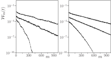
Figure 2: Distribution of harmonics ${\cal W}_{m}(t)$ as a function of $m$, at different times $t=10,30$ and $50$ from bottom to top (these curves are scaled by a factor 0.01, 0.1 and 1, respectively). Left and right panels correspond to pure ($\Delta=0$) and mixed ($\Delta=25$) initial states, see eq.(37). Other parameters of simulations are $g_{0}=2$, $\hbar=1$.

II.3.2 Complexity of a quantum state.

Just as it has been in the case of a classical phase space distribution, complexity of a quantum state can be characterized by the number $\langle|m|\rangle_{t}$ of $\theta$-harmonics of the Wigner function. The corresponding weights are given now by eqs. (42, 43) and again

$$\langle m^{2}\rangle_{t}=\sum_{m=0}^{\infty}m^{2}\,\mathcal{W}_{m}(t)=-\frac{\rm d^{2}F(\sigma;t)}{\rm d\sigma^{2}}\Big{|}_{\sigma=0}.$$ (44)

It should be emphasized that the chosen measure is equally valid in the quantum as well as classical cases. This allows direct comparison of the main features of the both dynamics. In particular, whereas the number of harmonics of the classical distribution function increases, due to the exponential instability, exponentially during the whole time of evolution, in the quantum case the exponential regime is, generally speaking, restricted to the Ehrenfest time interval. These statements are illustrated in the Fig.3 where the dependence of the quantity $\langle m^{2}\rangle_{t}$ on the time is shown for a set of different values of the effective Plank’s constant.

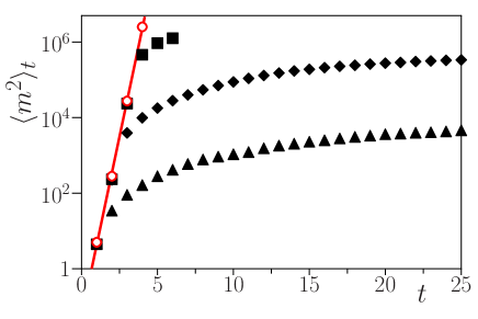
Figure 3: $\langle m^{2}\rangle_{t}$ before and after the Ehrenfest time. Triangles, diamonds and squares: $\hbar=1,\,0.1$ and $0.01$ respectively. Classical dynamics is shown by empty red circles, the gray line presents an exponential fit. The initial phase area holds constant $1/2$ in all 3 cases. The kick strength used here is $g_{0}=1.5$.

The Plank’s constant plays here a twofold role: on the one part it fixes the phase volume of the elementary quantum cell that is occupied in the phase space by the pure ground state ${\hat{\rho}}(0)=|0\rangle\langle 0|$, and, on the other part, it governs the dynamics via the evolution equation. In the Fig.3 we keep constant the size 1/2 of the initial Wigner distribution (38) by choosing $\Delta=1/2-\hbar/2$. The initial state is pure ($\Delta=0$) when $\hbar=1$ (triangles) but becomes more and more mixed ($\Delta\approx 1/2\gg\hbar$) in the cases $\hbar=0.1$ (diamonds) and $\hbar=0.01$ (squares) correspondingly. It is clearly seen that the smaller is the value of dynamical Plank’s constant the longer the classical exponential regime lasts. By other words, the mixing of the initial state suppresses the quantum interference effect and restores the classical behavior.

II.3.3 Information entropy vs von Neumann entropy

The probabilistic meaning of the quantities $\mathcal{W}_{m}(t)$ allows us to introduce the Shannon or information entropy:

$${\cal I}(t) = -\sum_{m=0}^{\infty}\mathcal{W}_{m}(t)\,\ln\mathcal{W}_{m}(t)$$ (45)

$$= \left\{\begin{array}[]{ll}0,&t=0,\\ \ln\langle|m|\rangle_{t}+1-\frac{\ln 2}{2}+O(1/\langle|m|\rangle_{t}),&\langle|m|\rangle_{t}\gg 1.\\ \end{array}\right.$$ (48)

This is another, though equivalent, possible way to characterize the complexity of a quantum state. Such a choice turns out to be even more convenient for our further purposes. This entropy starts from zero (the initial state has no harmonics but zero), increases linearly (with a slope defined by the classical characteristic time $\tau_{c}$) during the Ehrefest time and then slows down to the quantum logarithmic regime. Since the number of harmonics at sufficiently large time weakly depends on the peculiar properties of the initial state, being practically the same for pure and mixed ones, this entropy is practically insensitive to quantum correlations.

On the contrary, the invariant von Neumann entropy

$${\cal S}(t)=-\mathrm{Tr}\left[{\hat{\rho}}(t)\,\ln{\hat{\rho}}(t)\right]={\cal S}(0)$$ (49)

is perfectly sensitive to quantum correlations (hence the name ‘‘correlational’’ Sokol98 ). This entropy does not depend on time as long as the evolution remains unitary and equals zero ${\cal S}(t)=0$ when the state is pure. The coherence and quantum correlations can be destroyed only in the presence of an persistent external noise or during the process of preparation of the initial state (see below).

II.3.4 Persistent noise.

The stationary noise is described in our model by the Hamiltonian operator

$${\hat{H}}^{(noise)}({\hat{a}}^{{\dagger}},{\hat{a}};t)=\hbar\,{\hat{n}}\sum_{\tau}\xi_{\tau}\,\delta(t-\tau),\quad\langle\xi_{\tau}\rangle=0,\,\langle\xi_{\tau}\xi_{\tau^{\prime}}\rangle=\sigma^{2}\delta_{\tau\tau^{\prime}}\,.$$ (50)

As a result, the evolution operator takes the form

$$\hat{\cal U}(\{\xi\};t)=\prod_{\tau=1}^{\tau=t}\left[e^{-i\xi_{\tau}{\hat{n}}}\,\hat{U}\right].$$ (51)

This operator remains unitary for any fixed noise realization $\{\xi\}$ (history). Accordingly, a pure initial state remains pure during the whole time of evolution. At a running moment $t$, the excitation of the oscillator and the degree of anisotropy of the Wigner function are characterized by the probability distributions Sokol09

$$w_{n}({\xi};t)=\langle n|\hat{\rho}({\xi};t)|n\rangle,$$ (52)

and

$$\mathcal{W}_{m}(t)=\frac{(2-\delta_{m0})}{\mathbb{P}(t)}\sum_{n=0}^{\infty}\Big{|}\langle n+m\big{|}{\hat{\rho}}({\xi}t)\big{|}n\rangle\Big{|}^{2},\quad\,\sum_{m=0}^{\infty}\mathcal{W}_{m}(t)=1$$ (53)

where the density matrix

$$\hat{\rho}({\xi};t)=\hat{\cal U}(\{\xi\};t)\hat{\rho}(t=0)\hat{\cal U}^{\dagger}(\{\xi\};t)$$ (54)

is defined for some fixed noise realization $\{\xi\}$. The initial state can be chosen to be the ground one $\hat{\rho}(t=0)=\big{|}0\rangle\langle 0\big{|}$, because after a few first kicks the distributions (52,53) aquire a practically general exponential form (see Fig.4). Averaging over noise realizations keeps the slopes of these distributions unchanged but kills the wild fluctuations around their regular exponential decay. In the limit of strong noise $\sigma\gg 1$ (see thick dashed lines in Fig.4) the noise acts as a ‘‘coarse graining’’ that reproduces the behavior of the corresponding classical distributions Sokol09 . There exist "self-averaging" quantities like mean excitation number $\langle n\rangle_{t}$ or the mean number $\langle|m|\rangle_{t}$ of $\theta$-harmonics that do not depend, in fact, on the noise realization Sokol09

$$\langle n(\{\xi\};t)\rangle=n(\sigma;t),\,\,\,\langle m^{2}(\{\xi\};t)\rangle=m^{2}(\sigma;t)=n(\sigma;t)\left(n(\sigma;t)+1\right).$$ (55)

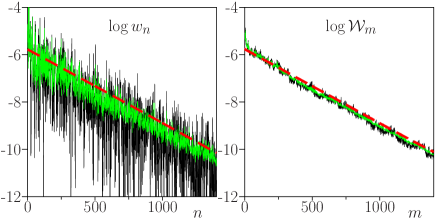
Figure 4: Probability distributions (52), (53) at the moment $t=80$ with no noise ($\sigma=0$, thin black lines), weak noise ($\sigma=0.001$, thin green lines) and strong noise ($\sigma=1$, thick dashed red line). In the two latter cases the distributions are averaged over $10^{3}$ realizations. The initial state is pure ($\Delta=0$, see eq.(37)). Other parameters of simulations are $g_{0}=2$, $\hbar=1$.

On the contrary, the quantum Peres fidelity defined as

$$F(\{\xi\};t)=\frac{\mathrm{Tr}\left[{\hat{\rho}(t)}\,{\hat{\rho}(\{\xi\};t)}\right]}{\mathbb{P}(t)}.$$ (56)

is not a self-averaging quantity and wildly fluctuates from one noise history to another. Therefore averaging over all possible noise realizations is necessary to obtain a reasonably simple and adequate measure:

$$F(\sigma;t)=\overline{F(\{\xi\};t)}^{\{\xi\}}=\mathrm{Tr}\left[{\hat{\rho}(t)}\,{\hat{\rho}^{(av)}(\sigma;t)}\right].$$ (57)

This procedure brings into consideration the average density matrix $\rho^{(av)}(t)$ whose one step evolution is described by the transformation

$$\langle n^{\prime}|{\hat{\rho}^{(av)}(\sigma;\tau)}|n\rangle=e^{-\frac{1}{2}\sigma^{2}(n^{\prime}-n)^{2}}\,\langle n^{\prime}|{\hat{U}}{\hat{\rho}^{(av)}(\sigma;\tau-1){\hat{U}}^{{\dagger}}}|n\rangle.$$ (58)

The noise suppresses off-diagonal matrix elements of the density matrix thus gradually cutting down the number of harmonics of the corresponding Wigner function. The evolution is not unitary anymore. The latter entails state mixing, loss of memory on the initial state and suppression of the quantum interference. These effects show up in the behavior of the von Neumann entropy defined in the terms of the averaged density matrix as

$${\cal S}(\sigma;t)=-\mathrm{Tr}\left[{\hat{\rho}}^{(av)}(\sigma;t)\,\ln{\hat{\rho}}^{(av)}(\sigma;t)\right].$$ (59)

The Fig.5 illustrates this behavior in comparison with that of the information Shannon entropy ${\cal I}(t)$ (see (45)). The entropy ${\cal S}(\sigma;t)$ increases the faster the larger is the level of noise (the full lines from bottom to top) and approaches the information Shannon ${\cal I}(\sigma;t)$ entropy (circles) from below. At some time $t_{(dec)}$, both the entropies coincide and go after that together. All coherent effects are washed away by this time. Therefore the entropy (59) is suitable for tracing the gradual loss of the quantum coherence.

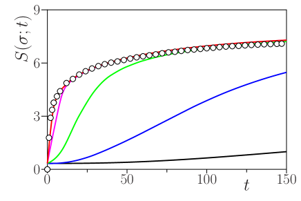
Figure 5: Von Neumann entropy: $\sigma=(0.125,1,8,64,512)\cdot 10^{-3}$, solid (black, blue, green, magenta, red) lines from bottom to top. Circles: information entropy ${\cal I}(t);\,\,\,{\cal S}(\sigma;t>t_{(dec)})\to{\cal I}(t)\,$. In these simulations we use $g_{0}=2$, $\hbar=1$.

The decoherence time $t_{(dec)}$ can be estimated as Sokol09

$$t_{(dec)}(\sigma)\thicksim\sqrt{\frac{\hbar}{\sigma^{2}D}}$$ (60)

where $D$ is the classical diffusion coefficient. Henceforth the system occupies the maximal phase area accessible at the running value of excitation thus reaching a sort of equilibrium. Finally, the system expands "adiabatically", the both entropies being almost constant. The further evolution turns out to be Markovian Sokol09 .

II.3.5 Time independent perturbation. Mixed initial state.

As it has already been noted above, the quantum interference turns out to be somewhat suppressed if the evolution started from a mixed initial state. We consider below another kind of decoherence that takes place in the case of a time-independent perturbation.

$$\hat{H}_{V}=\hat{H}^{(0)}+\varepsilon{\hat{V}},$$ (61)

where the unperturbed Hamiltonian describes, as before, dynamics of the classically chaotic nonlinear oscillator. The perturbed and unperturbed motions are juxtaposed by means of the unitary Loschmidt echo operator ${\hat{f}}(t)$ Sokol07

$${\hat{f}}(t) = {\hat{U}}^{{\dagger}}(t){\hat{U}}_{V}(t)$$ (62)

$${\hat{f}}(t) = T\exp\left[-i\frac{\varepsilon}{\hbar}\int_{0}^{t}d\tau{\hat{\cal V}}(\tau)\right]$$ (63)

$${\hat{\cal V}}(\tau) = {\hat{U}}^{{\dagger}}(t)\,{\hat{V}}{\hat{U}}(t).$$ (64)

In spite of the fact that the perturbation ${\hat{\cal V}}(\tau)$ evolves chaotically, the quantum coherence is in no way spoiled as long as the initial state is pure. More than that, one might think that even if the initial state is an incoherent mixture quantum coherence can be rapidly generated by producing complex off diagonal matrix elements during dynamical evolution. Nevertheless, we will show below that if the system is classically chaotic and the evolution starts from a wide incoherent mixed state, then the initial incoherence persists due to the intrinsic classical chaos so that the quantum phases remain irrelevant Sokol07 .

In the case of a pure initial state ${\hat{\rho}}(0)=|\overset{\circ}{\psi}\rangle\langle\overset{\circ}{\psi}|$ the Peres fidelity (13) is simply the probability

$$F_{\overset{\circ}{\psi}}(t)=|\langle\overset{\circ}{\psi}|{\hat{f}(t)}|\overset{\circ}{\psi}\rangle|^{2}=\left|\mathrm{Tr}\left[{\hat{f}(t)}\overset{\circ}{\rho}\right]\right|^{2}$$ (65)

to survive in this state under influence of a chaotically evolving perturbation ${\hat{\cal V}}(\tau)$ till the time $t$. When the evolution starts from a mixed state ${\hat{\rho}}(0)=\sum_{k}p_{k}|\overset{\circ}{\psi}_{k}\rangle\langle\overset{\circ}{\psi}_{k}|,\,\,\sum_{k}p_{k}=1$, the expression (65) can be generalized in two different ways. The first of them leads to the standard definition (13) that can be rewritten identically in the form

$$F(t)=\frac{1}{\mathrm{Tr}{\hat{\rho}^{2}(0)}}\sum_{k,k^{\prime}}p_{k}p_{k^{\prime}}W_{kk^{\prime}}(t)$$ (66)

where the quantities $W_{kk^{\prime}}(t)=|\langle\overset{\circ}{\psi}_{k}|{\hat{f}}(t)|\overset{\circ}{\psi}_{k^{\prime}}\rangle|^{2}$ are probabilities of transitions induced by the unitary transformation ${\hat{f}}(t)$. The influence of coherent effects is hidden in the dynamics of the complex matrix elements $f_{kk^{\prime}}(t)=\langle\overset{\circ}{\psi}_{k}|{\hat{f}}(t)|\overset{\circ}{\psi}_{k^{\prime}}\rangle$.

Another way of generalization is suggested by the experimental configuration with periodically kicked ion traps proposed in Gardi97 . In such Ramsey type interferometry experiments one directly accesses the fidelity amplitudes (see Gardi97 rather than their square moduli. Motivated by this consideration, we will consider further the quantity

$${\cal F}(t)=\left|\mathrm{Tr}\left[{\hat{f}(t)}{\hat{\rho}}(0)\right]\right|^{2}=\Big{|}\sum_{k}p_{k}f_{k}(t)\Big{|}^{2}=\sum_{k}p^{2}_{k}F_{k}(t)+\sum_{k,k^{\prime}}(1-\delta_{kk^{\prime}})p_{k}p_{k^{\prime}}f_{k}(t)f_{k^{\prime}}^{*}(t)\,,$$ (67)

that is obtained by directly extending the formula (65). Below we refer to this new quantity as allegiance. The first term in the r.h.s. is the sum of fidelities $F_{k}=|f_{k}|^{2}=|\langle\overset{\circ}{\psi}_{k}|{\hat{f}}|\overset{\circ}{\psi}_{k}\rangle|^{2}$ of the individual pure initial states with weights $p_{k}^{2}$, while the second, interference term, depends on the relative phases of fidelity amplitudes. If the number $K$ of pure states $|\overset{\circ}{\psi}_{k}\rangle$ that form the initial mixed state is large, $K\gg 1$, so that $p_{k}\backsimeq 1/K$ for $k\leqslant K$ and zero otherwise, the first term is $\backsim 1/K$ at the initial moment $t=0$ while the second term $\backsim 1$. Therefore, in the case of a wide mixture, the decay of the function ${\cal F}(t)$ is determined by the second sum of interfering contributions. Therefore, in contrast to the standard Peres fidelity (13, 66), the allegiance ${\cal F}$ directly accounts for the quantum interference and can be expected to retain quantal features even in the deep semiclassical region. This is not, however, the case as will be shown below.

Analytical calculation of the pure-state fidelity $F_{\overset{\circ}{\alpha}}(t)$ for a pure coherent quantum state $|\overset{\circ}{\alpha}\rangle$ as well as the allegiance ${\cal F}(t)$ for an incoherent mixed state can be performed with the help of expressing the both quantities in terms of the Feynman’s path integral in the oscillator’s phase plane. A method of semiclassical evaluation of this integral has been worked out in Sokol84 . Referring the reader to this paper for all technical details we present below the main results of the calculations Sokol07 .

These results are quite different it the two cases of our interest. If the initial state is a pure coherent one $|\overset{\circ}{\alpha}\rangle$ the fidelity amplitude is found to be

$$f_{\overset{\circ}{\alpha}}(t)=\frac{2}{\pi\hbar}\int d^{2}\delta\,e^{-\frac{2}{\hbar}|\delta|^{2}}\exp\left\{i\frac{\sigma}{2}\left[{\tilde{\theta}_{c}(t)}-{\overset{\circ}{\tilde{\theta}_{c}}}\right]\right\},$$ (68)

where the phase ${\tilde{\theta}_{c}(t)}=\theta_{c}(\omega_{0}-2|\delta|^{2};\overset{\circ}{\alpha}^{*}+\delta^{*},\overset{\circ}{\alpha}+\delta;t)=\int_{0}^{t}d\tau[\omega_{0}-2|\delta|^{2}+2{\tilde{I}}_{c}(\tau)$. It should be stressed that the fidelity $F_{\overset{\circ}{\alpha}}(t)=|f_{\overset{\circ}{\alpha}}(t)|^{2}$ does not decay in time at all if the quantum fluctuations described by the integral over $\delta$ in (68) are neglected.

On the initial stage of the evolution $t\ll\frac{1}{\Lambda}\ln\frac{2}{\varepsilon}$, while the phases ${\tilde{\theta}_{c}(t)}$ are not yet perfectly randomized the fidelity $F_{\overset{\circ}{\alpha}}$ decays, because of classical exponential instability, super-exponentially:

$$F_{\overset{\circ}{\alpha}}(t)\approx\exp\left(-\frac{\varepsilon^{2}}{4\hbar}e^{\Lambda t}\right),$$

Silve02 ; Iomin04 . During this time the contribution of the averaging over the initial Gaussian distribution in the classical $\overset{\circ}{\alpha}$ phase plane dominates while the influence of the quantum fluctuations of the linear frequency remains negligible. Such a decay has, basically, a classical nature Eckha03 and the Planck’s constant appears only as the size of the initial distribution. For larger times the quantum fluctuations reduce the fidelity decay to exponential law $F_{\overset{\circ}{\alpha}}(t)=\exp(-2\Lambda t).$

The situation changes dramatically if the initial state is an incoherent mixture. More precisely, we consider a mixed initial state represented by a Glauber’s diagonal expansion Glaub63 ; Glaub63a ${\hat{\rho}}(0)=\leavevmode\nobreak\ \int d^{2}\overset{\circ}{\alpha}{\cal P}(|\overset{\circ}{\alpha}-\overset{\circ}{\alpha}_{c}|^{2})|\overset{\circ}{\alpha}\rangle\langle\overset{\circ}{\alpha}|$ with a wide positive definite weight function ${\cal P}$ which covers a large number of quantum cells. Note that here and in the following we assume that the initial mixture is isotropically distributed in the phase plane around a fixed point $\overset{\circ}{\alpha}_{c}\,$, with the density ${\cal P}_{\overset{\circ}{\alpha}_{c}}(\overset{\circ}{\alpha}^{*},\overset{\circ}{\alpha})={\cal P}(|\overset{\circ}{\alpha}-\overset{\circ}{\alpha}_{c}|^{2})$. Then allegiance equals Sokol07 ${\cal F}(t;{\overset{\circ}{\alpha}_{c}})=|f(t;{\overset{\circ}{\alpha}_{c}})|^{2}$, where

$$\begin{array}[]{c}f(t;{\overset{\circ}{\alpha}_{c}})=\int d^{2}\overset{\circ}{\alpha}\,{\cal P}(|\overset{\circ}{\alpha}-\overset{\circ}{\alpha}_{c}|^{2})f_{\overset{\circ}{\alpha}}(t)\\ \approx\int d^{2}\overset{\circ}{\alpha}\,{\cal P}(|\overset{\circ}{\alpha}-\overset{\circ}{\alpha}_{c}|^{2})\exp\left\{i\frac{\varepsilon}{2\hbar}\left[\theta_{c}(t)-\overset{\circ}{\theta}_{c}(0)\right]\right\}.\end{array}$$ (69)

This formula directly relates the decay of a quantum quantity, the allegiance, to that of correlation function of the classical phases. No quantum features are present in the r.h.s. of (69).

Summarizing, the decay pattern of the allegiance ${\cal F}(t)$ depends on the value of the parameter $\sigma=\varepsilon/\hbar$. In particular, for $\sigma\ll 1$, we recover the well known Fermi Golden Rule (FGR) regime. Indeed, in this case the cumulant expansion can be used, $\ln f(t;{\overset{\circ}{\alpha}_{c}})=\sum_{\kappa=1}^{\infty}\frac{(i\sigma)^{\kappa}}{\kappa!}\chi_{\kappa}(t)\,.$ All the cumulants are real, hence, only the even ones are significant. The lowest of them,

$$\begin{array}[]{c}\chi_{2}(t)=\int_{0}^{t}d\tau_{1}\int_{0}^{t}d\tau_{2}\langle\left[I_{c}(\tau_{1})-\langle I_{c}(\tau_{1})\rangle\right]\left[I_{c}(\tau_{2})-\langle I_{c}(\tau_{2})\rangle\right]\rangle\equiv\int_{0}^{t}d\tau_{1}\int_{0}^{t}d\tau_{2}K_{I}(\tau_{1},\tau_{2})\;,\end{array}$$ (70)

is positive. Assuming that the classical autocorrelation function decays exponentially, $K_{I}(\tau_{1},\tau_{2})=\langle\left(\Delta I_{c}\right)^{2}\rangle\exp\left(-|\tau_{1}-\tau_{2}|/\tau_{I}\right)$ with some characteristic time $\tau_{I}$, we obtain $\chi_{2}(t)=2\langle\left(\Delta I_{c}\right)^{2}\rangle\tau_{I}t=2Kt$ for the times $t>\tau_{I}$ and arrive, finally, at the FGR decay law ${\cal F}(t;{\overset{\circ}{\alpha}}_{c})=\exp(-2\sigma^{2}Kt)$ Cerru02 ; Jacqu01 ; Prose02 . Here $K=\int_{0}^{\infty}d\tau K_{I}(\tau,0)=\langle\left(\Delta I_{c}\right)^{2}\rangle\tau_{I}\,.$

The significance of the higher connected correlators $\chi_{\kappa\geq 4}(t)$ grows with the increase of the parameter $\sigma$. When this parameter roughly exceeds one, the cumulant expansion fails and the FGR approximation is no longer valid. In the regime $\sigma\gtrsim 1$, the decay rate of the function ${\cal F}(t;{\overset{\circ}{\alpha}}_{c})=\big{|}f(t;{\overset{\circ}{\alpha}_{c}})\big{|}^{2}$ ceases to depend on $\sigma$ Sagde88 and coincides with the decay rate $1/\tau_{c}$ of the classical correlation function (19),

$${\cal F}(t;{\overset{\circ}{\alpha}}_{c})=\exp(-t/\tau_{c})\,.$$ (71)

This rate is intimately related to the local instability of the chaotic classical motion though it is not necessarily given by the Lyapunov exponent $\Lambda$ itself. Quantum interference does not show up at all.

II.4 Ballistic electron quantum transport in the presence of weakly disordered background.

Finally, we will discuss the decoherence phenomenon in the electron transport through an open ballistic quantum dot as this problem is seen from the point of view of the general resonance scattering theory Sokol10 . Peculiarities of this transport reflect the properties of eigenstates of the quantum billiards, whose spectra are highly nontrivial in the classicaly chaotic regimes.

The loss of coherence that is the main problem of our concern is attributed below to interaction with a weakly disordered many-body environment (‘‘walls’’). So, the whole our system consists of an open cavity and walls and is described by the following non-Hermitian effective Hamiltonian

$${\cal\hat{H}}=\left(\begin{array}[]{cc}{\cal H}^{(s)}&V^{{\dagger}}\\ V&H^{(e)}\\ \end{array}\right).$$ (72)

The upper left block stands for the non-Hermitian effective Hamiltonian of the irregularly shaped cavity (dot) with two similar leads supporting each $M/2$ equivalent channels.

$${\cal H}^{(s)}=H^{(s)}-\frac{i}{2}AA^{{\dagger}}$$ (73)

This non-Hermitian effective Hamiltonian describes a set of $N^{(s)}$ electron doorway resonance states with complex eigenenergies ${\cal E}_{n}=E_{n}-\frac{i}{2}\Gamma_{n}$ separated by mean level spacing $D$. The Hermitian matrix $H^{(e)}$ represents the environment with a very dense discrete spectrum of $N^{(e)}$ ($>>>N^{(s)}$) real energy levels $\epsilon_{e}$ (mean level spacing $\delta<<<D$). These states get excess to the continuum only due to the coupling $V$ to the doorway states in the cavity.

We exploit further the single particle approximation in the environmental sector: $H^{(e)}\Rightarrow H^{(e)}_{sp}$. The mean level spacing of a quasi-electron $d\propto 1/N^{(e)}_{sp}$ is much greater that the many-body spacing $\delta$ but still much smaller than the doorway spacing, $\delta\ll d\ll D$. The interaction $V$ with to irregular impurities is described by a rectangular $N^{(e)}_{sp}\times N^{(s)}$ matrix with random matrix elements

$$\langle V_{\nu n}\rangle=0,\quad\langle V_{\mu m}^{*}V_{\nu n}\rangle=\frac{1}{2}\Gamma_{s}\frac{d}{\pi}\delta_{\mu\nu}\delta_{mn}$$ (74)

The second relation defines the spreading width

$$\Gamma_{s}=2\pi\frac{\langle|V|^{2}\rangle}{d}$$ (75)

that satisfies the condition ${\Gamma_{s}}\gg d$, so that the influence of the disorder lies beyond validity of the standard perturbation theory.

The unitary $M\times M$ scattering matrix has the form

$$S(E)=I-i{\cal T}(E)=I-i{A^{{\dagger}}}{\cal G}_{D}(E)A.$$ (76)

Therefore the evolution of a scattered electron inside the cavity is described by the $(N^{(s)}\times N^{(s)})$ doorway resolvent (doorway propagator)

$${\cal G}_{D}(E)=\frac{I}{E-{\cal H}^{(s)}-\Sigma(E)}.$$ (77)

Here the Hermitian $N^{(s)}\times N^{(s)}$-matrix

$$\Sigma(E)=V^{{\dagger}}\frac{I}{E-H_{sp}^{(e)}}V=V^{{\dagger}}G_{sp}^{(e)}(E)V$$ (78)

accounts for transitions cavity $\leftrightarrow$ environment. Being averaged over the random coupling amplitudes $V$, this matrix is, with accuracy $1/N^{(e)}_{sp}$, diagonal and is proportional to the trace in the single-quasi-particle space.

$$\Sigma(E)\Rightarrow\frac{1}{2}{\Gamma_{s}}\,g(E);\quad g(E)=\frac{d}{\pi}TrG_{sp}^{(e)}(E).$$ (79)

As a result a given doorway resonance is fragmented in a large number of narrow resonances whose complex energies are found by solving the equation

$${\cal E}_{\nu}^{n}-{\cal E}_{n}-\frac{1}{2}\Gamma_{s}g({\cal E}_{\nu}^{n})=0,$$ (80)

so that $\Gamma_{s}/d$ fine structure resonances originate from any given doorway doorway state.

The transition matrix transforms now to

$${\cal T}^{ab}(E)=\sum_{n}\frac{{\cal A}_{n}^{a}{\cal A}_{n}^{b}}{E-{\cal E}_{n}-\frac{1}{2}{\Gamma_{s}}g(E)}=\sum_{\nu}\frac{\tilde{\cal A}_{\nu}^{a}\tilde{\cal A}_{\nu}^{b}}{E-{\cal E}_{\nu}}.$$ (81)

The resulting transition amplitudes are now sums of interfering contributions of all narrow fine-structure resonances. The new pole residues are complex and, therefore, interfere! No loss of coherence on this stage!

II.4.1 Time delay.

The resonant Smith time delay matrix $Q=-iS^{{\dagger}}dS/dE$ can be expressed Sokol97 in terms of the vectors $b^{(s,e)}$ of the intrinsic part of the total scattering wave function. A straightforward calculation gives $Q\!=\!{b^{(s)}}^{{\dagger}}b^{(s)}+{b^{(e)}}^{{\dagger}}b^{(e)}\!=\!Q^{(s)}+Q^{(e)}$ where the vectors

$$\quad b^{(s)}(E)={\cal G}^{(s)}_{\textsc{d}}(E)A^{(s)}\,;\quad b^{(e)}(E)=G_{sp}^{(e)}(E)Vb^{(s)}(E)$$ (82)

have dimensions $N^{(s)}\times M$ and $N_{sp}^{(e)}\times M$ respectively. The two contributions $Q^{(s,e)}$ correspond to the modified due to the interaction with the background time delay within the dot and delay because of the virtual transitions into the background. In particular, the diagonal elements of the resonant Smith matrix give the norms of the internal parts of the scattering wave function initiated in specific channels. Finally, the typical scattering duration called the Wigner delay time is represented by the following weighted-mean quantity

$$\tau_{W}(E)=\frac{1}{M}{\rm Tr}\,Q(E)\,.$$ (83)

After averaging over the interaction $V$ we arrive in the main approximation to

$$Q(E)=\Lambda(E)\,{b^{(s)}}^{{\dagger}}b^{(s)}=\Lambda(E)Q^{(s)}(E)\,;\quad\Lambda(E)=1+\frac{1}{2}\Gamma_{s}l^{(e)}\;(E)$$ (84)

where $l(E)$=$\frac{d}{\pi}$$\rm Tr$ $\left[{G_{sp}^{(e)}}^{{\dagger}}(E)G_{sp}^{(e)}(E)\right]$.

In fact, however, the spectrum of the fine-structure resonances is extremely dense so that this structure cannot be resolved experimentally. Only quantities averaged over some energy interval $d\ll\Delta E\ll D$ are observed.

$$\begin{array}[]{c}\overline{\sigma^{ab}(E)}=\frac{1}{\Delta E}\int_{E-\frac{1}{2}\Delta E}^{E+\frac{1}{2}\Delta E}dE^{\prime}\,\big{|}{\cal T}^{ab}(E^{\prime})\big{|}^{2}\,;\\ \overline{\tau_{W}(E)}=\frac{1}{\Delta E}\int_{E-\frac{1}{2}\Delta E}^{E+\frac{1}{2}\Delta E}dE^{\prime}\,\tau_{W}(E^{\prime})\,.\end{array}$$ (85)

Neglecting unobservable spectral fluctuations of the background we assume a rigid spectrum with equidistant levels $\epsilon_{\mu}\!=\!\varepsilon_{0}\!+\!\mu d\!$ (the picket fence approximation). One of the advantages of this uniform model is that the loop functions $g(E),l(E)$ can be calculated explicitly Sokol97

$$g(E)=\cot\left(\frac{\pi E}{d}\right)\,,\quad l(E)=\frac{\pi}{d}\sin^{-2}\left(\frac{\pi E}{d}\right)\,.$$ (86)

II.4.2 Isolated doorway resonance near the Fermi energy.

If the incoming electron with the energy $E\approx E_{res}$ excites an isolated ($\Gamma=\sum_{c}\Gamma^{c}\ll D$) resonance state with the energy $E_{res}\approx 0$ very close to the Fermi surface in the environment, the transition cross section turns out to be equal to

$$\sigma^{ab}(E)=\Big{|}{\cal T}^{ab}(E)\Big{|}^{2}=\frac{\Gamma^{a}\Gamma^{b}}{\left[E-\frac{1}{2}\Gamma_{s}\cot\left(\frac{\pi E}{d}\right)\right]^{2}+\frac{1}{4}\Gamma^{2}}\,,$$ (87)

when the Wigner time delay looks in this case as

$$\tau_{W}(E)=\Gamma\,\frac{1+\frac{\pi\Gamma_{s}}{2d}\sin^{-2}\left(\frac{\pi E}{d}\right)}{\left[E-\frac{1}{2}\Gamma_{s}\cot\left(\frac{\pi E}{d}\right)\right]^{2}+\frac{1}{4}\Gamma^{2}}\,.$$ (88)

The both quantities reveal strong fine-structure fluctuations on the typical scale of the background level spacing $d$.

The fine-scale energy averaging yields then

$$\overline{\sigma^{ab}(E)}=\frac{\Gamma^{a}\Gamma^{b}}{E^{2}+\frac{1}{4}\left(\Gamma+\Gamma_{s}\right)^{2}}+\frac{\Gamma^{a}\Gamma^{b}}{\Gamma}\frac{\Gamma_{s}}{E^{2}+\frac{1}{4}\left(\Gamma+\Gamma_{s}\right)^{2}}=\left(1+\frac{\Gamma_{s}}{\Gamma}\right)\frac{\Gamma^{a}\Gamma^{b}}{E^{2}+\frac{1}{4}\left(\Gamma+\Gamma_{s}\right)^{2}}\,\,.$$ (89)

The averaging destroyed the coherence and decomposed the cross section into a sum of two incoherent contributions. The first of them corresponds to excitation and subsequent decay of the doorway resonance (widened because of leaking into the environment) through one of the $M$ outer channels. The leakage effect is described by additional shift in the upper part of the complex energy plane by the distance $\frac{1}{2}\Gamma_{s}$. The second term accounts for the particles re-injected back in the cavity from the background. There is no net loss of the electrons. All of them escape finally via outer channels.

The environment looks from outside as a black box which swallows a particle and spits it back in the cavity after some time. This time is characterized by the mean Wigner time delay that also consists of two contributions,

$$\overline{\tau_{W}}(E)=\frac{\Gamma+\Gamma_{s}}{E^{2}+\frac{1}{4}(\Gamma+\Gamma_{s})^{2}}+\frac{2\pi}{d}\;.$$ (90)

The first term describes the delay on the damped by the internal ‘‘friction’’ resonance level inside the dot when the second one accounts for the electrons delayed in the environment by the time $\tau_{d}=\frac{2\pi}{d}$ proportional to the quasi-particle’s level density.

The conductivity of the device is proportional to the transport cross section

$$G(E) = \sum_{a\in 1,b\in 2}\overline{\sigma^{ab}(E)}=\frac{\Gamma_{1}\,\Gamma_{2}}{\Lambda(E)}+\frac{\Gamma_{1}\,\Gamma_{2}}{\Gamma_{1}+\Gamma_{2}}\,\frac{\Gamma_{s}}{\Lambda(E)}$$ (91)

$$= T_{12}+\frac{T_{1s}\,T_{s2}}{T_{1s}+T_{s2}}$$ (92)

where $\Gamma_{k}=\sum_{c\in k}\Gamma^{c}$, $k=1,2$; $\Gamma_{1}+\Gamma_{2}=\Gamma$ and

$$T_{sk}(E)=\frac{\Gamma_{s}\,\Gamma_{k}}{\Lambda(E)}\,,\quad\,\,\,\,\Lambda(E)=E^{2}+\frac{1}{4}\left(\Gamma+\Gamma_{s}\right)^{2}.$$ (93)

The term $T_{12}$ describes transition from the first to the second lead via the broadened intermediate doorway resonance when the additional contribution incorporates the interchanges with the environment. The latter can be naturally interpreted by introducing an additional fictitious $(M+1)th$ channel that connects the resonance state with the environment. The corresponding extended scattering matrix remains unitary.

The found expression is formally identical to that obtained within the framework of the Büttiker’s voltage-probe model Buetti86 ; Buetti88 of the decoherence phenomenon. The corresponding dimensionless decoherence rate equals in our case to $\gamma_{s}=\frac{2\pi}{D}\Gamma_{s}=\Gamma_{s}\tau_{D}$.

II.4.3 Many-body effects.

The single-particle approximation used up to now is well justified only when the scattering energy $E$ is very close to the Fermi surface in the environment. For higher scattering energies, many-body effects should be taken into account. They show up, in particular, in a finite lifetime of the quasi-electron with the energy $E>E_{F}=0$. The simplest way to account for this effect is to attribute some imaginary part to the quasi-particle’s energy, $\varepsilon_{\mu}=\mu d-\frac{i}{2}\Gamma_{e}$. The resonant denominator looks then as Sokol97

$${\cal D}_{res}(E)=E-E_{res}-\frac{1}{2}\Gamma_{s}(1-\xi^{2})\frac{\eta}{1+\xi^{2}\eta^{2}}+\frac{i}{2}\left(\Gamma+\Gamma_{s}\xi\frac{1+\eta^{2}}{1+\xi^{2}\eta^{2}}\right)$$ (94)

where $E_{res}$ is the position of the doorway resonance and the following notations

$$\xi=\tanh\left(\frac{\pi\Gamma_{e}}{2d}\right),\quad\eta=\cot\left(\frac{\pi E}{d}\right)$$

has been used. The transport cross section $G(E)$ retains still its form (91) but the subsidiary transition probabilities looks now as

$$T_{sk}(E)\Rightarrow T_{sk}(E;\kappa)=\frac{\Gamma_{s}\,\Gamma_{k}}{\Lambda(E;\kappa)}$$ (95)

instead of (93). The factor

$$\frac{1}{\Lambda(E;\kappa)}=\frac{1}{\Lambda(E)}\,\frac{1}{1+\kappa\frac{\Lambda(E)}{\Gamma\Gamma_{s}}},\quad\Lambda(E)=(E-E_{res})^{2}+\frac{1}{4}(\Gamma+\Gamma_{s})^{2}$$ (96)

depends on the new parameter $\kappa$ that accounts for inelastic effects in the background,

$$\begin{array}[]{c}\kappa=\frac{4\xi}{(1-\xi)^{2}}=e^{\gamma_{e}}-1\approx\\ \left\{\begin{array}[]{l}\gamma_{e}\ll 1,\,\,\,\,\,\,\,\textrm{if}\,\,\,\,\,\,\,\,\,\,{\tau}_{e}\gg\tau_{d}\,,\\ e^{\gamma_{e}}\gg 1,\,\,\,\,\,\textrm{if}\,\,\,\,\,\,\,\,\,\,\tau_{e}<\tau_{d}\,,\\ \end{array}\right.\quad(\gamma_{e}=\tau_{d}\Gamma_{e})\end{array}$$ (97)

where ${\tau}_{e}=1/\Gamma_{e}$ is the lifetime of the quasi-electron in the environment.

Strictly speaking, the assumed quasi-electron decay, that implies infinite density of the final states in the background, seems to destroys the unitarity of the scattering matrix in contradiction with what has been stated before. In fact, a single-particle state once excited in the environment with a very dense but, nevertheless, discrete spectrum evolves after that quite similar to a quasi-stationary state only till the time $2\pi/\delta\gg\tau_{e}=1/\Gamma_{e}$. After this time, recovery of the initial non-stationary state begins. An electron that carry in particular electric charge preserves to a certain extent its individuality in the environment. It can lose, because of the many-body effects, only a part of its energy but not the charge and inevitably returns sooner or later in the cavity and escapes finally via one of the outer channels. There exists a good probability for the electron to be re-emitted in the cavity with some intermediate energy $E_{out}<E_{in}\approx E_{res}$ within the much shorter time interval $\tau_{d}=\frac{2\pi}{d}$. The portion of energy lost by such a retarded electron dissipates inside the environment. As a result, the background temperature jumps slightly up during each act of the scattering. However, supposing that the environment system is bulky enough, we can disregard this very slow increase of the environment temperature. Alternatively, we can suppose that a special cooling technique is in use.

Near the doorway resonance energy $E_{res}$ the influence of the finite lifetime effects is negligible within the range $0\leqslant\kappa\lesssim\kappa_{c}=\frac{4\Gamma\Gamma_{s}}{(\Gamma+\Gamma_{s})^{2}}$. The critical value $\kappa_{c}$ reaches it’s maximum possible, $\kappa_{c}=1$, when $\Gamma=\Gamma_{s}$ and becomes small if one out of the two widths noticeably exceeds another. In these cases the interval of weak absorption is very restricted and the absorption begins to play an important role. If the resonance is so narrow that $\Gamma\ll\Gamma_{s}$, then $\kappa_{c}\approx 4\frac{\Gamma}{\Gamma_{s}}\ll 1$ and the subsidiary probabilities (95) at the resonance energy $E=E_{res}$ and $\kappa\gtrsim\kappa_{c}$ are small, $T_{sk}(E=E_{res};\kappa)\approx\frac{16}{\kappa}\frac{\Gamma\Gamma_{k}}{\Gamma_{s}^{2}}\lesssim\frac{16}{\kappa_{c}}\frac{\Gamma\Gamma_{k}}{\Gamma_{s}^{2}}\approx 4\frac{\Gamma_{k}}{\Gamma_{s}}\ll 1$. On the other hand, the very quasi-particle concept is self-consistent only if $\gamma_{e}=\tau_{d}\Gamma_{e}\lesssim 1$ so that the physically feasible interval of the strong absorption regime is $\kappa_{c}\approx 4\frac{\Gamma}{\Gamma_{s}}\lesssim\kappa\lesssim 1$. In this interval, the subsidiary transition probabilities (95) are much smaller than the direct transport probability $T_{12}$ thus signifying suppression of quantum coherence, the degree of suppression being quantitatively characterized by the decoherence rate $\gamma_{s}\equiv\frac{2\pi}{D}\Gamma_{s}$. Another possible method of accounting for the absorbtion has been proposed in Efeto95 . The absorption is modelled in this case by including in the Hamiltonian a spatially uniform imaginary potential with the strength $-\frac{i}{2}\gamma_{\phi}$. Results of this two approaches become equivalent with the obvious identification $\gamma_{\phi}=\gamma_{s}$.

II.4.4 Overlapping doorway resonances.

A number of overlapping doorway states can be excited if the incoming electron energy $E_{in}$ appreciably exceeds the Fermi energy. As before, the cross sections averaged over the fine structure scale consist of incoherent contributions of directly scattered and penetrated into the environment and then re-emitted particles.

$$\overline{\sigma^{{ab}}(E)}=\sigma_{d}^{ab}(E)+\sigma_{r}^{ab}(E),$$ (98)

where the direct and re-emitted contributions are

$$\sigma_{d}^{ab}(E) = \Big{|}\sum_{n}\frac{{\cal A}_{n}^{a}{\cal A}_{n}^{b}}{{\cal D}_{n}(E)}\Big{|}^{2},$$ (99)

$$\sigma_{r}^{ab}(E) = \Gamma_{s}\int_{0}^{\infty}dt_{r}\,\sigma_{r}^{ab}(E;t_{r}),$$ (102)

$$\sigma_{r}^{ab}(E;t_{r})=\Big{|}\sum_{n}\frac{{\cal A}_{n}^{a}{\cal A}_{n}^{b}}{{\cal D}_{n}(E)}\,e^{-i{\cal E}_{n}t_{r}}\Big{|}^{2},$$

$${{\cal D}_{n}(E)}=E-E_{n}+\frac{i}{2}\left(\Gamma_{n}+\Gamma_{s}\right).$$

The particles delayed within environment for different times contribute incoherently.

Since the electron motion in the cavity is supposed to be classically chaotic the ensemble averaging $\langle...\rangle$ in the doorway sector is appropriate. It is easy to see that, as long as the inelastic effects in the background are fully neglected, such an averaging perfectly eliminates dependence of all mean cross sections on the spreading width. Indeed, the ensemble averaged cross section is expressed in terms of the S-matrix two-point correlation function $C_{V}^{ab}(\varepsilon)=C_{0}^{ab}(\varepsilon-i\Gamma_{s})$ as

$$\langle\sigma_{d}^{ab}(E)\rangle=C_{V}^{ab}(0)=C_{0}^{ab}(-i\Gamma_{s})=\int_{0}^{\infty}dt\,e^{-\Gamma_{s}t}\,K_{0}^{ab}(t)\,.$$ (103)

The subscript $V$ indicates the coupling to the background and the function $K_{0}^{ab}(t)$ is the Fourier transform of the correlation function $C_{0}^{ab}(\varepsilon)$. On the other hand, it is easy to show that

$$\langle\sigma_{r}^{ab}(E;t_{r})\rangle=\int_{0}^{\infty}dt\,e^{-\Gamma_{s}t}\,K_{0}^{ab}(t+t_{r})\,.$$ (104)

Therefore, finally,

$$\begin{array}[]{c}\langle\overline{\sigma^{ab}(E)}\rangle=\int_{0}^{\infty}dt\,e^{-\Gamma_{s}t}\,K_{0}^{ab}(t)\\ +\Gamma_{s}\int_{0}^{\infty}dt_{r}\int_{0}^{\infty}dt\,e^{-\Gamma_{s}t}\,K_{0}^{ab}(t+t_{r})=\int_{0}^{\infty}dt\,\,K_{0}^{ab}(t)=\langle\sigma_{0}^{ab}(E)\rangle\,.\end{array}$$ (105)

The ensemble averaging, being in fact equivalent to the energy averaging over the doorway scale $D$, suppresses all interference effects save the elastic enhancement because of the time reversal symmetry. The latter effect manifests itself in the weak localization phenomenon. The time reversal symmetry is violated owing to the energy absorption in the environment.

II.4.5 Energy absorption and suppression of the weak localization.

Taking into account eq. (105) we rewrite the ensemble-averaged cross sections as $\langle\overline{\sigma^{ab}(E)}\rangle=\langle\sigma_{0}^{ab}(E)\rangle+\Delta\sigma^{ab}(E;\kappa)$ where the second contribution can be reduced Sokol10 to the following compact expression

$$\Delta\sigma^{ab}(E;\kappa)=-\sqrt{\frac{\kappa\Gamma_{s}}{4}}\int_{0}^{\infty}\frac{dt}{\sqrt{-\frac{d}{dt}+\frac{\kappa}{4\Gamma_{s}}\left(\frac{d}{dt}-\Gamma_{s}\right)^{2}}}\,K_{0}^{ab}(t)\,.$$ (106)

Being presented in such a form, this result is equally valid for both the orthogonal (GOE, time reversal symmetry) as well as the unitary (GUE, no time reversal symmetry) cases.

To simplify further calculation we will consider the case of an appreciably large number $M\gg 1$ of statistically equivalent scattering channels, all of them with the maximal transmission coefficient $T=1$. Then, first, the channel indices $a,b$ can be dropped. And, second, the characteristic decay time $t_{W}=1/\Gamma_{W}=\tau_{D}/M$ (this time is called the dwell time when the inverse quantity is known as the Weisskopf width) of the function $K_{0}(t)$ is much shorter than the mean delay time $\tau_{D}=2\pi/D$. Independently of time reversal symmetry, the function $K_{0}(t)$ is real, positive definite, monotonously decreases with time $t$ and satisfies the conditions $K_{0}(t<0)=0,\,\,K_{0}(0)=1$. This allows us to represent this function in the form of the mean-weighted decay exponent Sokol08b :

$$K_{0}(t)=\int_{0}^{\infty}d\Gamma\,e^{-\Gamma t}\,w(\Gamma),\quad\int_{0}^{\infty}d\Gamma\,w(\Gamma)=K_{0}(0)=1\,.$$ (107)

Rigorously speaking, the weight functions $w(\Gamma)$ have different forms before ($t<\tau_{D}$) and after ($t>\tau_{D}$) the Heisenberg time $\tau_{D}$. However contribution of the latter interval is as small as $e^{-M}$ Sokol08b . Neglecting such a contribution we obtain in any inelastic channel

$$\Delta\sigma(E;\kappa)=-\sqrt{\frac{\kappa\Gamma_{s}}{4}}\int_{0}^{\infty}d\Gamma\,\frac{w(\Gamma)}{\Gamma}\frac{1}{\sqrt{\Gamma+\frac{\kappa}{4\Gamma_{s}}(\Gamma+\Gamma_{s})^{2}}}\,.$$ (108)

In the strong absorption limit $\kappa\gg\frac{4\Gamma_{s}\Gamma_{W}}{(\Gamma_{s}+\Gamma_{W})^{2}}$ the parameter $\kappa$ disappears from the found expression and the latter reduces to

$$\Delta\sigma(E;\kappa)\Rightarrow-\Gamma_{s}\int_{0}^{\infty}d\Gamma\,\frac{w(\Gamma)}{\Gamma\,(\Gamma+\Gamma_{s})}=-\Gamma_{s}\int_{0}^{\infty}dt_{r}\int_{0}^{\infty}dt\,e^{-\Gamma_{s}t}\,K_{0}^{ab}(t+t_{r})\,.$$ (109)

According to Eqs. (103, 105) this brings us to the result

$$\langle\overline{\sigma(E)}\rangle=\int_{0}^{\infty}dt\,e^{-\Gamma_{s}t}\,K_{0}(t)=\int_{0}^{\infty}d\Gamma\frac{w(\Gamma)}{\Gamma+\Gamma_{s}}=\langle\sigma_{d}(E)\rangle.$$ (110)

The averaged cross section approaches in this limit the value $1/\Gamma_{s}$ independently of the symmetry class when the spreading width $\Gamma_{s}$ noticeably exceeds the typical widths contributing to the integral over $\Gamma$.

For the case of time reversal symmetry (GOE) the asymptotic expansion Verba85 of the two-point correlation function gives Sokol07

$$w^{(GOE)}(\Gamma)=\delta(\Gamma-\Gamma_{W})-\frac{2}{t_{H}}\delta^{\prime}(\Gamma-\Gamma_{W})+\frac{M}{2t_{H}^{2}}\delta^{\prime\prime}(\Gamma-\Gamma_{W})+...$$ (111)

whereas for the case of absence of such a symmetry (GUE) similar expansion result in

$$w^{(GUE)}(\Gamma)=\delta(\Gamma-\Gamma_{W})+...\,.$$ (112)

In both these cases contributions of the omitted terms are estimated as $O(1/(M^{-7/2}))$. With such an accuracy, the formula (108) yields for the weak localization the expression

$$\begin{array}[]{c}\Delta G\equiv G^{(GUE)}-G^{(GOE)}\\ =M_{1}M_{2}\left(2\frac{d}{d\mu}+\frac{\mu}{2}\frac{d^{2}}{d\mu^{2}}\right)\left\{\frac{1}{\mu}\left[1-\frac{\sqrt{\frac{\kappa\gamma_{s}}{4}}}{\sqrt{\mu+\frac{\kappa}{4\gamma_{s}}(\mu+\gamma_{s})^{2}}}\right]\right\}\Big{|}_{\mu=M}\\ \end{array}$$ (113)

which is valid for arbitrary values of the parameters $\kappa$, $\gamma_{s}$ and $M$. The unfolded explicit expression is a bit too lengthy. Visualization of this result is presented in Fig. 6 for two different values of the (dimensionless) spreading width $\gamma_{s}$ and $M_{1}=M_{2}=2;M=4$. The reduction of the difference $\Delta G$ displays suppression of the quantum coherence. Note that the effect becomes more pronounced as the number of channels decreases.

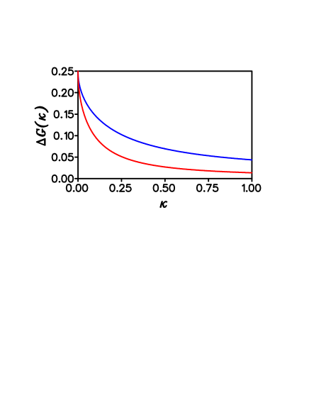
Figure 6: Weak localization versus absorption parameter $\kappa$. Lines correspond to $\gamma_{s}=25$ (blue) and $\gamma_{s}=64$ (red); $M=4$.

III Acknowledgments

We are very much obliged to Giuliano Benenti, Giulio Casati, and Yaroslav Kharkov with whom we had the advantage of cooperation over a period of years. V.V.S. is especially grateful to Vladimir Zelevinsky for long lasting friendship and collaboration. This work is supported by the Ministry of Education and Science of the Russian Federation (contract 14.B37.21.8408). Also we greatly appreciate countenance by the RAS Joint scientific program "Nonlinear dynamics and Solitons".

References

- [1] H. D. Abarbanel and J. D. Crawford. Strong coupling expansions for nonintegrable hamiltonian systems. Physica D: Nonlinear Phenomena, 5(2-3):307–321, Sep 1982.
- [2] G. Agarwal and E. Wolf. Calculus for functions of noncommuting operators and general phase-space methods in quantum mechanics. i. mapping theorems and ordering of functions of noncommuting operators. Physical Review D, 2(10):2161–2186, Nov 1970.
- [3] G. Agarwal and E. Wolf. Calculus for functions of noncommuting operators and general phase-space methods in quantum mechanics. ii. quantum mechanics in phase space. Physical Review D, 2(10):2187–2205, Nov 1970.
- [4] Y. Alhassid. The statistical theory of quantum dots. Reviews of Modern Physics, 72(4):895–968, Oct 2000.
- [5] H. Baranger and P. Mello. Mesoscopic transport through chaotic cavities: A random s-matrix theory approach. Physical Review Letters, 73(1):142–145, Jul 1994.
- [6] C. Beenakker. Random-matrix theory of quantum transport. Reviews of Modern Physics, 69(3):731–808, Jul 1997.
- [7] C. W. J. Beenakker and B. Michaelis. Stub model for dephasing in a quantum dot. Journal of Physics A: Mathematical and General, 38(49):10639–10646, Dec 2005.
- [8] G. Benenti, G. G. Carlo, and T. Prosen. Wigner separability entropy and complexity of quantum dynamics. Physical Review E, 85(5):051129, May 2012.
- [9] G. Benenti, G. Casati, and G. Veble. Decay of the classical loschmidt echo in integrable systems. Physical Review E, 68(3):036212, Sep 2003.
- [10] G. Benenti, G. Casati, and G. Veble. Stability of classical chaotic motion under a system’s perturbations. Physical Review E, 67(5):055202, May 2003.
- [11] E. Bogomolny. Smoothed wave functions of chaotic quantum systems. Physica D: Nonlinear Phenomena, 31(2):169–189, Jun 1988.
- [12] M. Büttiker. Role of quantum coherence in series resistors. Physical Review B, 33(5):3020–3026, Mar 1986.
- [13] M. Büttiker. Coherent and sequential tunneling in series barriers. IBM J. Res. Developm., 32:63–75, 1988.
- [14] N. Cerruti and S. Tomsovic. Sensitivity of wave field evolution and manifold stability in chaotic systems. Physical Review Letters, 88(5):054103, Jan 2002.
- [15] B. Chirikov. A universal instability of many-dimensional oscillator systems. Physics Reports, 52:263–379, 1979.
- [16] B. Eckhardt. Echoes in classical dynamical systems. Journal of Physics A: Mathematical and General, 36(2):371–380, Jan 2003.
- [17] K. Efetov. Temperature effects in quantum dots in the regime of chaotic dynamics. Physical Review Letters, 74(12):2299–2302, Mar 1995.
- [18] S. Gardiner, J. Cirac, and P. Zoller. Quantum chaos in an ion trap: The delta-kicked harmonic oscillator. Physical Review Letters, 79(24):4790–4793, Dec 1997.
- [19] R. Glauber. Coherent and incoherent states of the radiation field. Physical Review, 131(6):2766–2788, Sep 1963.
- [20] R. Glauber. Photon correlations. Physical Review Letters, 10(3):84–86, Feb 1963.
- [21] M. C. Gutzwiller. Chaos in Classical and Quantum Mechanics (Interdisciplinary Applied Mathematics) (v. 1). Springer, 1990.
- [22] F. Haake. Quantum Signatures of Chaos (Springer Series in Synergetics, Vol 54). Springer-Verlag, 1991.
- [23] E. Heller. Bound-state eigenfunctions of classically chaotic hamiltonian systems: Scars of periodic orbits. Physical Review Letters, 53(16):1515–1518, Oct 1984.
- [24] K. S. Ikeda. Time irreversibility of classically chaotic quantum dynamics. In G. Casati and B. Chirikov, editors, Quantum Chaos: Between Order and Disorder, pages 147–155. Cambridge University Press, 1995.
- [25] A. Iomin. Loschmidt echo for a chaotic oscillator. Physical Review E, 70(2):026206, Aug 2004.
- [26] F. M. Izrailev. Simple models of quantum chaos: Spectrum and eigenfunctions. Physics Reports, 196(5-6):299–392, Nov 1990.
- [27] P. Jacquod, P. Silvestrov, and C. Beenakker. Golden rule decay versus Lyapunov decay of the quantum loschmidt echo. Physical Review E, 64(5):055203(R), Oct 2001.
- [28] R. Jalabert, H. Baranger, and A. Stone. Conductance fluctuations in the ballistic regime: A probe of quantum chaos? Physical Review Letters, 65(19):2442–2445, Nov 1990.
- [29] C. Marcus, A. Rimberg, R. Westervelt, P. Hopkins, and A. Gossard. Conductance fluctuations and chaotic scattering in ballistic microstructures. Physical Review Letters, 69(3):506–509, Jul 1992.
- [30] L. Mehta. Random Matrices. Academic Press, 1991.
- [31] P. A. Mello, P. Pereyra, and T. H. Seligman. Information theory and statistical nuclear reactions. i. general theory and applications to few-channel problems. Annals of Physics, 161(2):254–275, May 1985.
- [32] A. Peres. Stability of quantum motion in chaotic and regular systems. Physical Review A, 30(4):1610–1615, Oct 1984.
- [33] T. Prosen and M. Znidaric. Stability of quantum motion and correlation decay. Journal of Physics A: Mathematical and General, 35(6):1455–1481, Feb 2002.
- [34] R. Z. Sagdeev, D. A. Usikov, and G. M. Zaslavsky. Nonlinear Physics: from pendulum to turbulence and chaos, volume 4. Harwood Academic, Chur, Switzerland, 1988.
- [35] P. G. Silvestrov and C. W. J. Beenakker. Ehrenfest times for classically chaotic systems. Phys. Rev. E, 65:035208(R), 2002.
- [36] V. Sokolov, G. Benenti, and G. Casati. Quantum dephasing and decay of classical correlation functions in chaotic systems. Physical Review E, 75(2):026213, Feb 2007.
- [37] V. Sokolov, B. Brown, and V. Zelevinsky. Invariant correlational entropy and complexity of quantum states. Physical Review E, 58(1):56–68, Jul 1998.
- [38] V. Sokolov and V. Zelevinsky. Simple mode on a highly excited background: Collective strength and damping in the continuum. Physical Review C, 56(1):311–323, Jul 1997.
- [39] V. Sokolov, O. Zhirov, G. Benenti, and G. Casati. Complexity of quantum states and reversibility of quantum motion. Physical Review E, 78(4):046212, Oct 2008.
- [40] V. V. Sokolov. Moments of the distributio function and kinetic equation for stochastic motion of a nonlinear oscillator. Theoretical and Mathematical Physics, 59(1):396–403, Apr 1984.
- [41] V. V. Sokolov. On the nature of the quantum corrections in the case of stochastic motion of a nolinear oscillator. Theoretical and Mathematical Physics, 61(1):1041–1048, Oct 1984.
- [42] V. V. Sokolov. Decay rates statistics of unstable classically chaotic systems. In NUCLEI AND MESOSCOPIC PHYSICS: Proc. Int. Workshop on Nuclei and Mesoscopic Physics WNMP 2007, volume 995 of AIP Conf. Proc., pages 85–91. American Institute of Physics, American Institute of Physics, 2008. East Lansing, Michigan, 20-22 October 2007.
- [43] V. V. Sokolov. Ballistic electron quantum transport in the presence of a disordered background. Journal of Physics A: Mathematical and Theoretical, 43(26):265102, Jul 2010.
- [44] V. V. Sokolov and O. V. Zhirov. How well a chaotic quantum system can retain memory of its initial state? EPL (Europhysics Letters), 84(3):30001, Nov 2008.
- [45] V. V. Sokolov, O. V. Zhirov, and Y. A. Kharkov. Quantum dynamics against a noisy background. EPL (Europhysics Letters), 88(6):60002, Dec 2009.
- [46] J. Verbaarschot, H. Weidenmüller, and M. Zirnbauer. Grassmann integration in stochastic quantum physics: The case of compound-nucleus scattering. Physics Reports, 129(6):367–438, Dec 1985.
- [47] G. Zaslavsky. Chaos in Dynamic Systems. Routledge, 1985.
- [48] W. H. Zurek. Decoherence, einselection, and the quantum origins of the classical. Reviews of Modern Physics, 75(3):715, 2003.