Shockwave Compression and Joule-Thomson Expansion

Abstract

Structurally-stable atomistic one-dimensional shockwaves have long been simulated by injecting fresh cool particles and extracting old hot particles at opposite ends of a simulation box. The resulting shock profiles demonstrate tensor temperature, $T_{xx}\neq T_{yy}$ and Maxwell’s delayed response, with stress lagging strainrate and heat flux lagging temperature gradient. Here this same geometry, supplemented by a short-ranged external “plug” field, is used to simulate steady Joule-Kelvin throttling flow of hot dense fluid through a porous plug, producing a dilute and cooler product fluid.

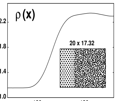
Figure 1: A typical shockwave snapshot. The motion is left-to-right with hot fluid exiting at the right boundary. Density snapshot uses Lucy’s weight function.

Stationary One-Dimensional Shockwaves—Shockwaves are arguably farther from equilibrium than are any other readily available states of a nonequilibrium fluidb1 ; b2 ; b3 ; b4 ; b5 ; b6 ; b7 ; b8 ; b9 . In just a few collision times, or mean free paths, the shock transforms cold equilibrium fluid (or solid) into a hot compressed stateb1 ; b2 ; b3 ; b4 ; b5 . Laboratory shockwaves at a few terapascals can compress condensed matter as much as threefold, to densities and pressures far greater than those at the center of the earthb6 . Because the shock transformation is a steady small-scale continuous process, converting kinetic energy to internal energy without any external heating, steady-state shockwave structures can be replicated with computer simulationsb2 ; b3 ; b4 ; b5 ; b7 ; b8 ; b9 . The inset of Figure 1 shows an interior snapshot of a typical simulation, with cold particles entering at the left and hot ones exiting to the right. The corresponding density profile snapshot using Lucy’s weight function for the spatial averagingb7 ; b8 ; b9 ; b10 ; b11 is the smooth curve. The shockwidth can be estimated from the maximum slope. It is just a few atomic spacings. Steady-state profiles generated in this way are fully consistent with the transient profiles generated with [1] shrinking periodic boundaries or [2] headon collisions of two similar blocks of cold materialb5 ; b7 ; b8 ; b9 .

Both experiments and simulations show that initially-sinusoidal shockfronts soon become planar. Steady shockwaves are accurately one-dimensionalb3 ; b5 ; b7 . Accordingly, the mass, momentum, and energy fluxes ( in the $x$ direction, the propagation direction ) are all constant in the comoving coordinate frame of Figure 1, the frame moving with the shockwaveb1 :

$$\left\{\ \rho u\ ;\ P_{xx}+\rho u^{2}\ ;\ (\rho u)[\ e+(P_{xx}/\rho)+(u^{2}/2)\ ]+Q_{x}\ \right\}\ ;\ {\rm All\ Three\ Fluxes\ Constant}\ .$$

Here $\rho(x)$ and $u(x)$ are the mass density and the flow velocity, $P_{xx}(x)$ is the pressure-tensor component in the propagation direction. $e(x)$ is the internal energy per unit mass and $Q_{x}$ is the heat flux vector, measuring the conductive flow of heat in the comoving frame.

The cold entrance velocity is $+u_{s}$ (the “shock velocity”) and the hot exit velocity is $+(u_{s}-u_{p})$ (where $u_{p}$ is the “particle velocity”) in the hot fluid. Away from the shockfront the cold and hot pressure and energy have their thermodynamic equilibrium values :

$$P_{xx}(x)\longrightarrow P_{\rm eq}\ ;\ e(x)\longrightarrow e_{\rm eq}\ .$$

Eliminating $u_{s}$ and $u_{p}$ from the three constant-flux equations gives the “Hugoniot Equation” or “shock adiabat”, $\Delta e=P\Delta v\$, where $P$ is the mean pressure, $[\ P_{\rm cold}+P_{\rm hot}\ ]/2$ , and $\Delta v$ is the overall change in volume per unit mass, $(1/\rho)_{\rm cold}-(1/\rho)_{\rm hot}$. Though there is no external heating there is heat flow within the shockwave structure. For weak shockwaves it is given by Fourier’s Law, $Q_{x}=-\kappa(dT/dx)$ .

The limiting values of the energy flux divided by the mass flux far from the shockwave are equal :

$$[\ e+(P/\rho)+(u_{s}^{2}/2)\ ]_{\rm cold}=[\ e+(P/\rho)+(1/2)(u_{s}-u_{p})^{2}\ ]_{\rm hot}\ .$$

In shockwaves the inflow is supersonic so that the kinetic energy cannot be ignored. Choosing the initial thermodynamic state along with the particle velocity determines the shock velocity as well as the pressure and energy of the resulting “hot” state.

Joule-Thomson “Throttling” Flows—In the 1850s Joule and Thomson (who became Lord Kelvin in 1892) collaborated on the design and analysis of experiments seeking to quantify the “mechanical equivalent of heat”. The “Joule-Thomson”, or “Joule-Kelvin”, experiment enforced the throttling of a high-pressure gas through a porous plug. A detailed description of the evolution of these experiments can be found in Reference 14 . Within the plug the inlet pressure is reduced to the smaller outlet pressure. As the flow rate approaches zero the experiment becomes isenthalpic, where the enthalpy is $E+PV$. Because there is no external heat flow the work added at the hot high-pressure side less that extracted on the cold low-pressure side is the energy change :

$$[\ e+(P/\rho)\ ]_{\rm high\ P}\stackrel{{\scriptstyle\rightarrow}}{{=}}[\ e+(P/\rho)\ ]_{\rm low\ P}\ .\ {\rm[\ Joule-Thomson\ ]}$$

By contrast to the supersonic shockwave experiment kinetic energy is negligible in the typical laboratory Joule-Kelvin experiment. The conductive heat flux (a maximum at the shock front) is likewise invisible in the throttling experiment, concealed by the irreversible details of the porous plug. Otherwise, the geometry and the thermodynamics and the constancy of the fluxes look identical to the usual one-dimensional shockwave analyses. In both experiment types there is necessarily a positive entropy change within the flow, as is required by the Second Law of Thermodynamics.

Joule-Thomson Simulations—The structural similarity of shockwave compression and Joule-Kelvin expansion experiments suggests the possibility of simulating Joule-Kelvin flows with molecular dynamics. Here we validate and illustrate that idea. Our model must incorporate a computational “porous plug” to slow compressed input fluid. Pores, holes, and confining passageways come to mind. But a little reflection suggests a simpler approach—erecting a smooth potential-energy barrier perpendicular to the flow. This approach is successful. Apart from the entrance and exit boundaries, the motion is entirely conservative and Newtonian. The entrance internal energy can be controlled by adding $y$ displacements and/or Maxwellian velocities $(v_{x}-u,v_{y})$ to particles as they enter.

Near the potential plug barrier an anisotropic far-from-equilibrium state results. The fluid is first slowed and then accelerated normal to the barrier, with the result that the pressure and temperature are briefly anisotropic with $P_{xx}>P_{yy}$ and $T_{xx}>T_{yy}$ . The details of the equilibration involve the same Maxwellianb13 time delays seen in shockwaves.

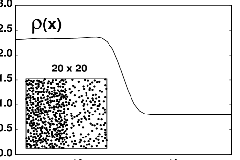
Figure 2: A Joule-Thomson snapshot. The motion is left-to-right with cooled fluid exiting at the right boundary. The density snapshot uses Lucy’s weight function, $(5/12)(1+|x|)[1-(|x|/3)]^{3}$ .

Figure 3: Time-averaged pressure tensor, velocity, and temperature tensor (left); time-averaged mass, momentum, and energy fluxes (right). The system dimensions are $200\times 40$ . The mass flux of unity is imposed by the rate at which fresh particles are inserted at the left boundary.

Figure 2 shows a typical Joule-Thomson steady-state particle snapshot, with similar pair and barrier potentials chosen to minimize integration errors using fourth-order Runge-Kutta molecular dynamics with a timestep $dt=0.01$ :

$$\phi_{\rm pair}(r<1)=[\ 1-r^{2}\ ]^{4}\ ;\ \phi_{\rm barrier}(-1<x<+1)=(1/4)[\ 1-x^{2}\ ]^{4}\ .$$

Although such a potential was perfectly satisfactory for the shockwave simulations of twofold compression it suggests the possibility of poor behavior at high density, where the force is a decreasing function of compression. Accordingly we compared results with a modified pair potential for which the force remains constant, with its maximum value $F_{\rm max}$ at separations less than $r_{\rm max}=\sqrt{(1/7)}=0.377964473$ :

$$\phi_{\rm max}(r<r_{\rm max})=(6/7)^{4}+F_{\rm max}(r-r_{\rm max})\ ;\ F_{\rm max}(r<r_{\rm max})=8(6/7)^{3}\sqrt{(1/7)}\ .$$

Joule-Thomson profiles including this $\phi_{\rm pair}$ precaution weren’t significantly changed from those with the unmodified potential.

Corresponding time-averaged density and velocity profiles are shown in Figure 3, along with the (necessarily constant) mass flux, $\rho u$ . Just as in our shock work the one-dimensional grid-profile averages were all computed using Lucy’s one-dimensional smooth-particle weight functionb7 ; b8 ; b9 ; b10 ; b11 , with $h=3$ :

$$\langle\ f(x_{g})\ \rangle=\sum_{x_{j}>x_{g}-h}^{x_{j}<x_{g}+h}f_{j}w_{gj}\ ;\ w_{gj}=(5/12)[\ 1+|x_{gj}|\ ][\ 1-(|x_{gj}|/3)\ ]^{3}\rightarrow\int_{-3}^{+3}w(|x|)dx\equiv 1\ .$$

With an input speed of 0.5, which quickly accelerates to 0.62, the velocity speeds up to 1.25 on passing through the plug potential. Straightforward Runge-Kutta simulation converges relatively simply and quickly to a flow satisfying slight modifications of the conservation relations which hold for shockwave simulations.

The longitudinal momentum flux drops at the barrier because the barrier force removes momentum. The overall flux drop exactly matches $(F_{\rm barrier}/L_{y})$ , with

$$[\ P+\rho u^{2}\ ]_{\rm left}=[\ P+\rho u^{2}\ ]_{\rm right}-(F/L_{y})\ [\ F\ {\rm negative}\ ]\ .$$

Mass, momentum, and energy fluxes are shown in Figure 3.

The energy flux is particularly interesting. Adding the contributions of pair interactions $(\frac{\dot{x}_{i}+\dot{x}_{j}}{2})x_{ij}F^{x}_{ij}$ to the “convective flux” gives perfect agreement between the entrance and exit flows. These contributions can be divided equally between Particles $i$ and $j$. Alternatively, they can be velocity-weighted: $(\frac{\dot{x}_{i}}{2})x_{ij}F^{x}_{ij}$ for $i$ and $(\frac{\dot{x}_{j}}{2})x_{ij}F^{x}_{ij}$ for $j$. The effect of this choice on the energy flux is insignificant, of order $0.001$. In shockwaves the total pressure-tensor component $P_{xx}$ includes the $\rho kT_{xx}$ which is absent in our Joule-Thomson flux. The derivations for these two slightly different expressions for the energy flux are both familiar textbook fareb15 . The reason for the difference is interesting. The $x$ component of the purely kinetic part of the energy flux (excluding the contributions from $\phi$ and $F$) involves local sums cubic in the velocity components. In the equilibrium case the cubic sum can be expressed in terms of the stream velocity and the deviations from it, which can in turn be expressed in terms of temperature :

$$\langle\ (v_{x}/2)(v_{x}^{2}+v_{y}^{2})\ \rangle=(1/2)\langle\ (u+\delta v_{x})^{3}+u(\delta v_{y})^{2}\ \rangle=(1/2)u^{3}+(3/2)ukT_{xx}+(1/2)ukT_{yy}\ .$$

The resulting “extra” $\rho ukT_{xx}$ can, if desired, be combined with the potential part of $uP_{xx}$ so as to agree with the continuum energy-flux expression. Far from equilibrium this simplification does not hold and the full cubic kinetic-theory sums must be evaluated.

In general, it is interesting to note that the hot and cold momentum fluxes don’t match in the Joule-Kelvin experiment though they do in the shockwave. (If both the fluxes, energy and momentum, were to match, either the shockwave or the throttling experiment would violate the Second Law!) The reason for the flux drop at the barrier is the latter’s contribution to the momentum flux, by exerting a nonzero compressive force on the hot fluid. In our demonstration problem the fluid is cooled substantially, in keeping with the familiar commercial mechanism using throttling as a model refrigerator. Like shockwaves, the present high-speed Joule-Thomson flows are contained by equilibrium thermodynamic boundaries. A series of Joule-Thomson states can be generated by using several plug barriers rather than just one. Accordingly, we believe that they will, like shockwaves, provide a useful source of computer-experimental constitutive information for flow states far from equilibrium and help in choosing the optimum weight function for correlating microscopic and macroscopic flow descriptions.

References

- (1) L. D. Landau and E. M. Lifshitz, Fluid Mechanics (Pergamon Press, New York, 1959). Chapter IX is devoted to shockwaves.
- (2) R. E. Duff, W. H. Gust, E. B. Royce, M. Ross, A. C. Mitchell, R. N. Keeler, and W. G. Hoover, “Shockwave Studies in Condensed Media”, in Behavior of Dense Media under High Dynamic Pressures, Proceedings of the 1967 Paris Conference, pages 397-406 (Gordon and Breach, New York, 1968).
- (3) V. Y. Klimenko and A. N. Dremin, “Structure of Shockwave Front in a Liquid”, pages 79-83 in Detonatsiya, Chernogolovka (Akademia Nauk, Moscow, 1978).
- (4) Wm. G. Hoover, “Structure of a Shockwave Front in a Liquid”, Physical Review Letters 42, 1531-1534 (1979).
- (5) Brad Lee Holian, Wm. G. Hoover, Bill Moran, and Galen K. Straub, “Shockwave Structure via Nonequilibrium Molecular Dynamics and Navier-Stokes Continuum Mechanics”, Physical Review A 22, 2798-2808 (1980).
- (6) C. E. Ragan, III, “Shockwave Experiments at Threefold Compression”, Physical Review A 29, 1391-1402 (1984).
- (7) Wm. G. Hoover and Carol G. Hoover, “Tensor Temperature and Shockwave Stability in a Strong Two-Dimensional Shockwave”, Physical Review E 80, 011128 (2009).
- (8) Wm. G. Hoover, Carol G. Hoover, and Francisco J. Uribe, “Flexible Macroscopic Models for Dense-Fluid Shockwaves: Partitioning Heat and Work; Delaying Stress and Heat Flux; Two-Temperature Thermal Relaxation” [ ariv:1005.1525 ].
- (9) Wm. G. Hoover and Carol G. Hoover, Computer Simulation, Time Reversiblity, Algorithms, and Chaos (World Scientific Publishing, Singapore, 2012). Chapter 6 is devoted to shockwaves.
- (10) L. B. Lucy, “A Numerical Approach to the Testing of the Fission Hypothesis”, The Astronomical Journal 82, 1013-1024 (1977).
- (11) Wm. G. Hoover, Smooth Particle Applied Mechanics—The State of the Art (World Scientific Publishers, Singapore, 2006).
- (12) William Thomson, “On the Thermal Effects of Fluids in Motion”, Philosophical Transactions of the Royal Society of London 143, 357-365 (1853).
- (13) J. C. Maxwell, “On the Dynamical Theory of Gases”, Philosophical Transactions of the Royal Society of London 157, 49-88 (1867).
- (14) J. S. Rowlinson, “James Joule, William Thomson and the Concept of a Perfect Gas”, Notes and Records of the Royal Society 64, 43-57 (2010).
- (15) Wm. G. Hoover, Molecular Dynamics (Springer-Verlag, Berlin, 1986), available without charge at [ http://williamhoover.info ] . See Sections II.B and II.C.