Mode spectrum and temporal soliton formation
in optical microresonators

Abstract

The formation of temporal dissipative solitons in optical microresonators enables compact, high repetition rate sources of ultra-short pulses as well as low noise, broadband optical frequency combs with smooth spectral envelopes. Here we study the influence of the resonator mode spectrum on temporal soliton formation. Using frequency comb assisted diode laser spectroscopy, the measured mode structure of crystalline MgF₂ resonators are correlated with temporal soliton formation. While an overal general anomalous dispersion is required, it is found that higher order dispersion can be tolerated as long as it does not dominate the resonator’s mode structure. Mode coupling induced avoided crossings in the resonator mode spectrum are found to prevent soliton formation, when affecting resonator modes close to the pump laser. The experimental observations are in excellent agreement with numerical simulations based on the nonlinear coupled mode equations, which reveal the rich interplay of mode crossings and soliton formation.

Temporal dissipative solitons Lugiato and Lefever (1987); Wabnitz (1993); Leo et al. (2010) can be formed in a Kerr-nonlinear optical microresonator Herr et al. (2012a) with anomalous dispersion that is driven by a monochromatic continuous wave pump laser. These temporal solitons are sech²-shaped ultra-short pulses of light circulating inside the microresonator, where the temporal width of the solitons is fully determined by the resonator dispersion and nonlinearity as well as the pump power and pump laser detuning Herr et al. (2012a); Coen and Erkintalo (2013). It has been shown that the pump laser parameters can be used to control the number of solitons circulating in the microresonator. In particular the single soliton state, where one single soliton is circulating continuously inside the resonator, is of high interest for applications. In the time domain soliton formation in microresonators allows for the generation of periodic ultra-short femto-second pulses, which in the frequency domain correspond to a frequency comb spectrum with smooth sech²-shaped spectral envelope. The free spectral range (FSR) of the resonator, typically in the range of tens to hundreds of GHz, determines the pulse repetition rate (equivalent to the frequency comb line spacing). Soliton formation is related to four-wave mixing based frequency comb generation in microresonators Del’Haye et al. (2007); Savchenkov et al. (2008); Grudinin et al. (2009); Razzari et al. (2010); Levy et al. (2010); Foster et al. (2011); Papp and Diddams (2011); Kippenberg et al. (2011); Liang et al. (2011); Wang et al. (2013), where low and high noise operating regimes Ferdous et al. (2011); Papp and Diddams (2011); Herr et al. (2012b) have been identified. Here, techniques such as $\delta-\Delta$-matching Herr et al. (2012b), self-injection locking Li et al. (2012); Haye et al. (2013) or parametric seeding Papp et al. (2013) can be used to achieve low noise operation. In contrast to these low noise four-wave mixing based combs (also termed Kerr combs), the transition to the soliton regime Herr et al. (2012b) offers a unique combination of features, such as intrinsic low noise performance, direct pulse generation in the microresonator Peccianti et al. (2012); Herr et al. (2012a); Saha et al. (2013), and smooth spectral envelope as shown in Figure 1. These properties are critical to applications in e.g. telecommunications Levy et al. (2012); Wang et al. (2012); Pfeifle et al. (2013), low phase noise microwave generation Savchenkov et al. (2004); Li et al. (2012), precision spectroscopy as well as frequency metrology Udem et al. (2002); Cundiff and Ye (2003).

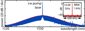
Figure 1: Measured optical spectrum with smooth sech²-shaped spectral envelope (red line) of a single temporal soliton generated in a continuous wave laser driven crystalline high-finesse MgF₂ microresonator. The spectral 3-dB width of 13 nm (1.62 THz) corresponds to a soliton pulse duration of 194 fs (full width at half maximum). The cw pump power is $\sim 3$0 mW at a wavelength of 1552 nm. The inset shows the resolution bandwidth (RBW) limited RF signal at a frequency of 14.09 GHz corresponding to the soliton pulse repetition rate.

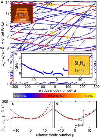
Figure 2: (a) Mode structure of a MgF₂ resonator with linewidths in the range of 50 to 500 kHz and an approximate FSR of 14.09 GHz, as measured by frequency comb assisted diode laser spectroscopyDel’Haye et al. (2009). Dots forming a continuous line represent a particular mode family. Different free spectral ranges correspond to different slopes of the lines, whereas dispersion and variation of the free spectral range show as curvature and bending of the lines. The dispersion can be strongly affected by mode crossings. Four specific mode families have been numbered by yellow labels. The color codes the measured resonance depth and helps to track particular mode families. (b) Comparable measurement of the fundamental TM11 mode in a Si₃N₄ microresonator with a resonator linewidth of $350$ MHz and approximate FSR of 76 GHz (consisting of a 800 nm high and 2 $\mu$m wide Si₃N₄waveguide embedded in SiO₂). The mode family shows signs of mode coupling to other mode families. (c) Illustration of higher order dispersion with $D_{3}>0$. The gray line indicates anomalous dispersion described by $D_{2}$ only. (d) Illustration of mode coupling induced mode frequency shift altering the dispersion properties locally. A simple parametrization using magnitude $a$ and position $b$ of the avoided mode crossing can be used for numerical modeling.

Temporal dissipative solitons in microresonators rely on the balance between Kerr-nonlinearity and anomalous group-velocity dispersion in the presence of a monochromatic pump laser and loss. Theory predicts that soliton formation is possible in any Kerr-nonlinear microresonator with anomalous dispersion for sufficiently high pump power Leo et al. (2010); Matsko et al. (2011); Herr et al. (2012a); Coen et al. (2013); Chembo and Menyuk (2013); Lamont et al. (2013). While high effective Kerr-nonlinearity and efficient non-linear frequency conversion is routinely achieved in a wide variety of resonator materials and geometries Del’Haye et al. (2007); Savchenkov et al. (2008); Grudinin et al. (2009); Razzari et al. (2010); Levy et al. (2010); Foster et al. (2011); Papp and Diddams (2011); Kippenberg et al. (2011); Liang et al. (2011); Wang et al. (2013), soliton formation has so far only been unambiguously demonstrated in MgF₂ microresonators Herr et al. (2012a) where the characteristic spectral sech²-shape envelope has been observed (cf. Figure 1). In this work we show that the decisive requirement for the generation of solitons is the anomalous resonator dispersion, which, in state of the art resonators, is affected by higher order dispersion and coupling of the optical modes Carmon et al. (2008); Del’Haye et al. (2009); Savchenkov et al. (2012); Grudinin et al. (2013). Understanding the formation of temporal dissipative solitons in the context of a complex mode-structure is not only an interesting and open scientific question, but essential to reliably reproduce soliton formation in other microresonator platforms such as SiN Levy et al. (2010); Foster et al. (2011).

The dispersion of a microresonator can be described in terms of its resonance frequencies $\omega_{\mu}$ using the parameters $D_{1}$, $D_{2}$, $D_{3}$ etc., which correspond to the free spectral range (FSR) in radians, the second order dispersion and higher order dispersion parameters, respectively Savchenkov et al. (2011); Herr et al. (2012b)

$$\omega_{\mu}=\omega_{0}+D_{1}\mu+\tfrac{1}{2}D_{2}\mu^{2}+\tfrac{1}{6}D_{3}\mu^{3}+...\hskip 10.00002pt.$$ (1)

Here, $\mu$ denotes the relative mode number with respect to the pump (designated by $\mu=0$). The parameter $D_{2}$ is related to the often employed group velocity dispersion (GVD) parameter $\beta_{2}$ via

$$D_{2}=-\frac{c}{n}D_{1}^{2}\beta_{2}\hskip 10.00002pt.$$ (2)

A positive $D_{2}$ corresponds to an anomalous resonator dispersion leading to a parabolic deviation of the resonance frequencies from an equidistant $D_{1}$-spaced grid (cf. grey curve in Figure 2c,d). This anomalous dispersion can be modified by higher order terms such as $D_{3}$ as illustrated schematically in Figure 2c. The dispersion coefficients $D_{2}$, $D_{3}$, etc. are typically estimated either analytically Schiller (1993); Gorodetsky and Ilchenko (1994); Gorodetsky and Fomin (2006, 2007); Demchenko and Gorodetsky (2013) or numerically Oxborrow (2007); Del’Haye et al. (2009); Riemensberger et al. (2012); Saha et al. (2012) by taking material and the geometrical dispersive effect into account. It is well known, that the coupling (e.g. via scattering) between mode families can additionally modify the mode frequencies Carmon et al. (2008); Del’Haye et al. (2009); Savchenkov et al. (2012); Grudinin et al. (2013) and lead to avoided crossings (illustrated schematically in Fig. 2d). In a simplified model the effect of a mode-crossing can be parametrized by its magnitude $a$ and position $b$ (details below). To investigate the dispersion requirements for soliton formation in an experimental system, broadband frequency comb assisted scanning laser spectroscopy Del’Haye et al. (2009) is used to precisely characterize the complex mode structure of a MgF₂ microresonator (FSR 14.09 GHz) Liang et al. (2010); Grudinin et al. (2012); Wang et al. (2013) over a spectral span exceeding 8 THz (including more than 600 FSR and several tens of mode families). From the recorded, frequency comb calibrated transmission spectra the resonance frequencies are determined. The measured mode structure is visualized in Figure 2 using a 2-dimensional representation. Here for each detected mode family and relative mode number $\mu$, the mode frequency is given with respect to a common equidistant frequency grid with a spacing of $\tilde{D_{1}}/2\pi=14.095$ GHz (close to the approximate average FSR, but chosen arbitrarily). The high number of optical modes and their complex mode-structure allow for investigation of different regimes of resonator dispersion and deriving empirical criteria for soliton formation.

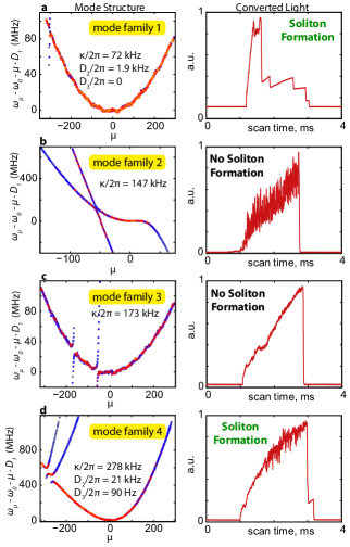
Figure 3: Experimental investigation of soliton formation in different dispersion scenarios in a MgF₂ microresonator. (a and d) Soliton formation is observed in the resonance families 1 and 4 of Figure 1, which show an almost ideal $D_{2}>0$ dominated anomalous dispersion. The soliton formation is detected by observation of the step signature in the converted light signal. (b and c) Soliton formation is not observed in the mode families 2 and 3 where strong deviations from $D_{2}$ dominated dispersion are present. The coupled pump power is $\mathcal{O}(1\mathrm{mW)}$ at a wavelength of 1552 nm.

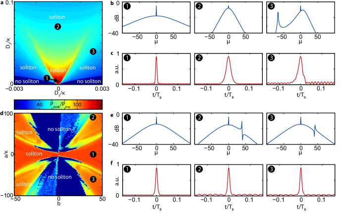
Figure 4: Numerical investigation of soliton formation in different dispersion scenarios. (a) The ratio $P_{\mathrm{peak}}/P_{\mathrm{avg}}$ of peak to average intracavity power is used as an indicator of soliton formation (which results in high peak power) for different combinations of $D_{2}$ and $D_{3}$. (b) Optical spectra for different parameters simulated in panel a (1,2,3) show narrow spectral width for high values of $D_{2}$ and asymmetric spectra, as well as dispersive wave phenomena (peak at $\mu=-65$), for nonzero $D_{3}$. (c) Temporal field envelope inside the microresonator corresponding to the spectra shown in panel b. The soliton pulse duration lengthens for larger values of $D_{2}$. Oscillatory features in the background field appear for nonzero $D_{3}$. (d) The high ratio of peak to average power is used as an indicator of soliton formation for different situations characterized by an avoided mode crossings that is parametrized by magnitude $a$ and distance $b$ from the pump laser (cf. Figure 2d). (e) Optical spectra for different simulation parameters in panel d (1,2,3) show the characteristic ’up-down’ feature induced by an avoided mode-crossing. (f) Temporal field envelope inside the microresonator corresponding to panel e. The pulses have the same duration but oscillatory features in the background field appear in the presence of avoided mode crossings.

Mode families with different free spectral range (corresponding to different radial and meridional mode numbers) that cross other mode families or that show modified dispersion due to avoided mode crossings can be observed. Some mode families exhibit normal other mode families anomalous dispersion. Moreover, mode coupling can locally alter the dispersion characteristics of a mode. The inset in Figure 2 shows that the effects of interacting modes are not only present in the case of a crystalline MgF₂ microresonator but also occur in a Si₃N₄ microresonator that due to its small cross-section supports only few higher order modes.

Next, the dispersion of four individual mode families is related to their potential of supporting temporal solitons. All four mode families allow for efficient non-linear frequency conversion. The latter is measured by detecting the parametrically frequency-converted laser light (i.e. the out-coupled optical comb spectrum with the pump wavelength filtered out, using a narrow-band fiber-Bragg grating) with a photo-detector. The converted light signal also provides direct means of detecting soliton formation. The latter exploits the fact that the formation of solitons coincides with discrete steps in the converted light signal (cf. Figure 3a,d, right column) that are observed when the pump laser is scanned over the resonance (see supplementary information in ref. Herr et al. (2012a)). The signals of the converted laser light for the four pumped modes ($\mu=0$) are shown in Figure 3 (right column) as function of the scan time. Despite significant nonlinear frequency conversion (and associated formation of comb-like broadband spectra) in all four mode families, only two mode families (1 and 4) exhibit soliton formation. To understand the reason, the dispersion properties of all four modes are investigated in detail based on the data shown in Figure 2a. Figure 3 (left column) shows the deviation of the resonance frequencies of the individual mode families from an equidistant frequency grid defined by the FSR (i.e. $D_{1}/2\pi$) of the mode family at the pumped resonance $\mu=0$. A perfectly anomalous dispersion, i.e. $D_{2}>0$ and vanishing higher order dispersion terms correspond to a convex, parabolic curve. This case is closely realized for mode family 1 ($D_{2}/2\pi=1.9$ kHz, $D_{3}/2\pi\approx 0$), which also shows the characteristic step signature Herr et al. (2012a) of soliton formation in Figure 3. Mode family 2 (Figure 3b) is not characterized by an anomalous dispersion and does not show signs of soliton formation. Mode family 3 (Figure 3c) exhibits an overall anomalous dispersion that is however disturbed locally by two avoided mode-crossings in the spectral proximity of the pumped mode. As a result no solitons are formed. In contrast, solitons are generated in mode family 4 (Figure 3d), which in addition to a dominating anomalous dispersion ($D_{2}/2\pi=21$ kHz) is characterized by a noticeable higher order contribution to its dispersion ($D_{3}/2\pi=90$ Hz). Moreover, the smooth dispersion curve is disturbed by two avoided mode crossings well separated in terms of mode number from the pumped mode. These measurements reveal that the formation of soliton is robust against a certain contribution of higher order dispersion as well as local mode frequency shift induced by mode coupling. However, an overall dispersion that is not generally anomalous (as in the case of mode family 2) or avoided mode-crossings too close to the pumped mode (as in the case of mode family 3) does prevent soliton formation. Note that a high optical finesse (i.e. narrow linewidth) is not a decisive requirement for soliton formation. Indeed the two soliton generating mode families (1 and 4) posses intermediate linewidths of $\kappa/2\pi=72$ kHz and 173 kHz compared to the mode families that do not support soliton formation (2 and 3) where $\kappa/2\pi=147$ kHz and 278 kHz. In short, the above experiments, correlating soliton formation with broadband precision dispersion mesurements, suggest that higher order dispersion and avoided mode-crossing are features that can prevent soliton formation. In the following we utilize numerical simulations to test and substantiate this experimentally motivated hypothesis.

The nonlinear physics in optical microresonators can be accurately modeled in the time or frequency domain, or via split-step methods combining both domains. Here we employ a split-step method implemented as an extension to the non-linearly coupled modes approachChembo and Yu (2010); Chembo and Menyuk (2013); Hansson et al. (2014). A key advantage of this method is that it allows for the definition of arbitrary mode frequencies $\omega_{\mu}$, enabling complex mode-structures to be readily simulated. To investigate whether a particular mode structure $\omega_{\mu}$ ($\mu=0,\pm 1,...$) allows for soliton formation, pump laser scans that can lead to the formation of solitons Herr et al. (2012a) are numerically simulated. To ensure deterministic computational evolution into a single soliton state the unperturbed analytical single soliton waveform Herr et al. (2012a) is used for seeding the simulation. For each simulated pump laser scan the maximum ratio of peak to average power inside the microresonator is computed. This ratio serves as a reliable indicator of soliton formation inside the microresonator. Throughout the simulation typical microresonator parameters of $\kappa/2\pi=1$ MHz, a FSR of $35$ GHz (roundtrip time $T_{R}\approx 29$ ps), an effective nonlinearity of $\gamma=4\times 10^{-4}$m^-1W^-1 and a pump power of $100$ mW at 1.55 $\mu$m wavelength are assumed. However all the simulations were performed in dimensionless units Herr et al. (2012a) and may be rescaled to other required sets of parameters.

First, to study the effect of higher order dispersion the optical modes are defined according to Equation 1 with varying $D_{2}$ and $D_{3}$ (Note that the offset $\omega_{0}$ and the linear term $D_{1}$ can be chosen arbitrarily). The numerical results in Figure 4a,b,c show that nonzero values of $D_{3}$ require a minimal magnitude of the coefficient $D_{2}$ to allow for soliton formation (consistent with our experimental observations). The maximum soliton peak intensities and shortest soliton pulse durations are achieved for vanishing $D_{3}$ and small values of $D_{2}>0.$ Figure 4a is a contour plot of the peak resonator intensities as a function of $D_{2}$ and $D_{3}$. It can be noted that the peak intensities are invariant under change of sign in $D_{3}$. The higher order dispersion $D_{3}$ causes the optical spectrum to become asymmetric and in the simulation is seen to result in dispersive wave formation Erkintalo et al. (2012); Coen et al. (2013); Lamont et al. (2013).

Second, the effect of avoided mode-crossings is studied in a simplified model. Here the mode frequencies are defined according to

$$\omega_{\mu}=\omega_{0}+D_{1}\mu+\tfrac{1}{2}D_{2}\mu^{2}+\frac{a/2}{\mu-b-0.5}$$ (3)

to phenomenologically mimic the effect of resonance frequency shifts induced by an avoided mode crossing. The parameters $a$ and $b$ specify the magnitude of this frequency shift and distance of the frequency from the pumped mode (cf. Figure 2d). Subtracting the value $0.5$ in the denominator of Equation 3 avoids an infinite mode shift for $\mu=b.$ As a result the maximum resonance frequency shift of $a$ occurs for the modes with modes numbers $\mu=b$ and $\mu=b+1$ towards smaller and higher frequency, respectively (The validity of the simple model has been verified in much slower direct simulation of mode coupling between two separate mode families, which led to similar results). The results of the simulations for various values of $a$ and $b$ are shown in Figure 4d,e,f. Here, Figure 4d shows the peak power as a function of the strength and location of the mode crossing. The contour plot exhibits a point symmetry, reflecting the equivalence of the mode shifts defined by $\{+a,+b\}$ and $\{-a,-b\}$, respectively. While Figure 4d reveals a rich and complex structure, it shows that generally, the larger the spectral separation $b$ of the mode crossing from the pumped mode ($\mu=0$), the higher the magnitude $a$ of the mode crossing can be without preventing soliton formation. The presence of crossing manifests itself in the optical spectrum as characteristic features,where the spectral intensities are increased on one side of the avoided crossing and decreased on the other cf. Figure 4e, trace 2 and 3 Grudinin et al. (2013). These features are evidenced experimentally in Figure 1c. Increasing the magnitude of the mode-crossing $a$ to larger values eventually inhibits the formation of solitons, in agreement with the experimental observations.

In summary, we have shown experimentally and numerically that a $D_{2}$ dominated anomalous resonator dispersion as well as a low number of mode crossings are essential prerequisites to the generation of temporal dissipative solitons in microresonators. A low number of avoided mode crossings can be achieved by reducing mode coupling and by designing single mode resonators.

Acknowledgements: This work was supported by the European Space Agency (V.B), a Marie Curie IIF (J.D.J), the Swiss National Science Foundation (T.H.), the Eurostars program and the DARPA QuASAR program, RFBR grant 13-02-00271 and state contract 07.514.12.4032 (M.L.G). The research leading to these results has received funding from the European Union Seventh Framework Programme (FP7/2007-2013) under grant agreement no. 263500.

References

- Lugiato and Lefever (1987) L. A. Lugiato and R. Lefever, Physical Review Letters 21, 2209 (1987).
- Wabnitz (1993) S. Wabnitz, Optics Letters 18, 601 (1993).
- Leo et al. (2010) F. Leo, S. Coen, P. Kockaert, S.-P. P. Gorza, P. Emplit, and M. Haelterman, Nature Photonics 4, 471 (2010).
- Herr et al. (2012a) T. Herr, V. Brasch, J. D. Jost, C. Y. Wang, N. M. Kondratiev, M. L. Gorodetsky, and T. J. Kippenberg, arXiv 1211.0733 (2012a).
- Coen and Erkintalo (2013) S. Coen and M. Erkintalo, Optics Letters 38, 1790 (2013).
- Del’Haye et al. (2007) P. Del’Haye, A. Schliesser, O. Arcizet, T. Wilken, R. Holzwarth, and T. Kippenberg, Nature 450, 1214 (2007).
- Savchenkov et al. (2008) A. A. Savchenkov, A. B. Matsko, V. S. Ilchenko, I. Solomatine, D. Seidel, and L. Maleki, Physical Review Letters 101, 93902 (2008).
- Grudinin et al. (2009) I. S. Grudinin, N. Yu, and L. Maleki, Optics Letters 34, 878 (2009).
- Razzari et al. (2010) L. Razzari, D. Duchesne, M. Ferrera, R. Morandotti, S. Chu, B. E. Little, and D. J. Moss, Nature Photonics 4, 41 (2010).
- Levy et al. (2010) J. S. Levy, A. Gondarenko, M. A. Foster, A. C. Turner-Foster, A. L. Gaeta, and M. Lipson, Nature Photonics 4, 37 (2010).
- Foster et al. (2011) M. A. Foster, J. S. Levy, O. Kuzucu, K. Saha, M. Lipson, and A. L. Gaeta, Optics Express 19, 14233 (2011).
- Papp and Diddams (2011) S. B. Papp and S. A. Diddams, Physical Reveiw A 84, 53833 (2011).
- Kippenberg et al. (2011) T. J. Kippenberg, R. Holzwarth, and S. A. Diddams, Science 332, 555 (2011).
- Liang et al. (2011) W. Liang, A. A. Savchenkov, A. B. Matsko, V. S. Ilchenko, D. Seidel, and L. Maleki, Optics Letters 36, 2290 (2011).
- Wang et al. (2013) C. Wang, T. Herr, P. Del’Haye, A. Schliesser, J. Hofer, R. Holzwarth, T. Hänsch, N. Picqué, and T. Kippenberg, Nature Communications 4, 1345 (2013).
- Ferdous et al. (2011) F. Ferdous, H. Miao, D. E. Leaird, K. Srinivasan, J. Wang, L. Chen, L. T. Varghese, and A. M. Weiner, Nature Photonics 5, 770 (2011).
- Herr et al. (2012b) T. Herr, K. Hartinger, J. Riemensberger, C. Y. Wang, E. Gavartin, R. Holzwarth, M. L. Gorodetsky, and T. J. Kippenberg, Nature Photonics 6, 480 (2012b).
- Li et al. (2012) J. Li, H. Lee, T. Chen, and K. J. Vahala, Physical Review Letters 109, 233901 (2012).
- Haye et al. (2013) P. D. Haye, S. B. Papp, and S. A. Diddams, arXiv 1307.4091, 1 (2013).
- Papp et al. (2013) S. B. Papp, P. D. Haye, and S. A. Diddams, arXiv 1305.3262 (2013).
- Peccianti et al. (2012) M. Peccianti, A. Pasquazi, Y. Park, B. E. Little, S. T. Chu, D. J. Moss, and R. Morandotti, Nature Communications 3, 765 (2012).
- Saha et al. (2013) K. Saha, Y. Okawachi, B. Shim, J. S. Levy, M. A. Foster, R. Salem, A. R. Johnson, M. R. E. Lamont, M. Lipson, and A. L. Gaeta, Optics Express 21, 1335 (2013).
- Levy et al. (2012) J. S. Levy, K. Saha, Y. Okawachi, M. a. Foster, A. L. Gaeta, and M. Lipson, IEEE Photonics Technology Letters 24, 1375 (2012).
- Wang et al. (2012) P.-H. Wang, F. Ferdous, H. Miao, J. Wang, D. E. Leaird, K. Srinivasan, L. Chen, V. Aksyuk, and A. M. Weiner, Optics Express 20, 29284 (2012).
- Pfeifle et al. (2013) J. Pfeifle, M. Lauermann, D. Wegner, V. Brasch, T. Herr, K. Hartinger, J. Li, D. Hillerkuss, R. Schmogrow, R. Holzwarth, et al., arXiv 1307.1037 (2013).
- Savchenkov et al. (2004) A. A. Savchenkov, A. B. Matsko, D. Strekalov, M. Mohageg, V. S. Ilchenko, and L. Maleki, Physical Review Letters 93, 243905 (2004).
- Udem et al. (2002) T. Udem, R. Holzwarth, and T. W. Hänsch, Nature 416, 233 (2002).
- Cundiff and Ye (2003) S. T. Cundiff and J. Ye, Reviews of Modern Physics 75, 325 (2003).
- Del’Haye et al. (2009) P. Del’Haye, O. Arciezt, M. L. Gorodetsky, R. Holzwarth, and T. J. Kippenberg, Nature Photonics pp. 529–533 (2009).
- Matsko et al. (2011) A. B. Matsko, A. A. Savchenko, W. Liang, V. S. Ilchenkko, S. D., and L. Maleki, Optics Letters 36, 2845 (2011).
- Coen et al. (2013) S. Coen, H. G. Randle, T. Sylvestre, and M. Erkintalo, Optics Letters 38, 37 (2013).
- Chembo and Menyuk (2013) Y. K. Chembo and C. R. Menyuk, Physical Reveiw A 87, 053852 (2013).
- Lamont et al. (2013) M. R. E. Lamont, Y. Okawachi, and A. L. Gaeta, Optics Letters 38, 3478 (2013).
- Carmon et al. (2008) T. Carmon, H. G. L. Schwefel, L. Yang, M. Oxborrow, A. D. Stone, and K. J. Vahala, Physical Review Letters 100, 103905 (2008).
- Savchenkov et al. (2012) A. A. Savchenkov, A. B. Matsko, W. Liang, V. S. Ilchenko, D. Seidel, and L. Maleki, Optics Express 20, 27290 (2012).
- Grudinin et al. (2013) I. S. Grudinin, L. Baumgartel, and N. Yu, arXiv 1309.4488, 1 (2013).
- Savchenkov et al. (2011) A. A. Savchenkov, A. B. Matsko, W. Liang, V. S. Ilchenko, D. Seidel, and L. Maleki, Nature Photonics 5, 293 (2011).
- Schiller (1993) S. Schiller, Applied Optics 32, 2181 (1993).
- Gorodetsky and Ilchenko (1994) M. L. Gorodetsky and V. S. Ilchenko, Optics Communications 113, 133 (1994).
- Gorodetsky and Fomin (2006) M. Gorodetsky and A. E. Fomin, IEEE Journal of Selected Topics in Quantum Electronics 12, 33 (2006).
- Gorodetsky and Fomin (2007) M. L. Gorodetsky and A. E. Fomin, Quantum Electronics 37, 167 (2007).
- Demchenko and Gorodetsky (2013) Y. A. Demchenko and M. L. Gorodetsky, Journal of the Optical Society of America B 30, 3056 (2013).
- Oxborrow (2007) M. Oxborrow, IEEE Transactions on Microwave Theory and Techniques 55, 1209 (2007).
- Riemensberger et al. (2012) J. Riemensberger, K. Hartinger, T. Herr, V. Brasch, R. Holzwarth, and T. J. Kippenberg, Optics Express 20, 770 (2012).
- Saha et al. (2012) K. Saha, Y. Okawachi, J. S. Levy, R. K. W. Lau, K. Luke, M. A. Foster, M. Lipson, and A. L. Gaeta, Optics Express 20, 26935 (2012).
- Liang et al. (2010) W. Liang, V. S. Ilchenko, A. A. Savchenko, A. B. Matsko, D. Seidel, and L. Maleki, Optics Letters 35, 2822 (2010).
- Grudinin et al. (2012) I. S. Grudinin, L. Baumgartel, and N. Yu, Optics Express 20, 6604 (2012).
- Chembo and Yu (2010) Y. K. K. Chembo and N. Yu, Physical Reveiw A 82, 33801 (2010).
- Hansson et al. (2014) T. Hansson, D. Modotto, and S. Wabnitz, Optics Communications 312, 134 (2014).
- Erkintalo et al. (2012) M. Erkintalo, Y. Q. Xu, S. G. Murdoch, J. M. Dudley, and G. Genty, Physical Reveiw Letters 109, 223904 (2012).