Preventing blue sky catastrophe in an array of $N$ identical Van-der-Pol oscillators coupled through nonlinear coupling

Preventing Blow-ups through Dynamic Random Links

Taming Blow-ups through Dynamic Random Links

Taming Explosive Growth through Dynamic Random Links

Abstract

We study the dynamics of a collection of nonlinearly coupled limit cycle oscillators, relevant to systems ranging from neuronal populations to electrical circuits, under coupling topologies varying from a regular ring to a random network. We find that the trajectories of this system escape to infinity under regular coupling, for sufficiently strong coupling strengths. However, when some fraction of the regular connections are dynamically randomized, the unbounded growth is suppressed and the system always remains bounded. Further we determine the critical fraction of random links necessary for successful prevention of explosive behaviour, for different network rewiring time-scales. These results suggest a mechanism by which blow-ups may be controlled in extended oscillator systems.

Collections of coupled dynamical systems were introduced as simple models capturing the essential features of large interactive systems cml . Research focussed around such distributed systems and complex networks has provided frameworks for understanding spatiotemporal patterns in problems ranging from Josephson junction arrays and multimode lasers, to microfluidic arrays and evolutionary biology ex1_cml -ex4_cml .

In this work we study the dynamics of a collection of nonlinearly coupled oscillators, relevant to systems ranging from neuronal populations to electrical circuits, under coupling topologies varying from a regular ring to a random network. We find that the trajectories of this system escape to infinity under regular coupling, for sufficiently strong coupling strengths, i.e. the amplitude of the oscillators grow explosively without bound. We term this phenomenon a blow-up. The surprising central result of this work is the following: when some fraction of the regular connections in this system are dynamically randomized, this unbounded growth is suppressed. Namely, random links successfully reign in the blow-ups in this complex dynamical network.

This counter-intuitive result is significant in the general context of taming infinities, as infinities arising in theoretical constructs of physical phenomena deeply concern scientists across disciplines popular . When physical quantities tend to infinite values in a model, it is often considered an indication of the failure of a theory, or symptoms of the limitations of the modelling. Removing infinities, for instance through theoretical tools such as renormalization, or through improvement of the underlying model of the physical process, has had much impact on physics in general. Further, from the point of view of potential applications, it is indeed crucial that no quantity grows without bound. So the drive to find mechanisms that can quell infinities in measurable quantities, stems from both methodological and pragmatic motivations popular . Specifically then, our observations in this work may yield methods to control and prevent blow-ups in extended oscillator systems, which are widely employed in a multitude of engineered devices. Lastly note that a certain degree of randomness in spatial links may be closer to physical reality, in many systems of biological, technological and physical significance Watts . So our finding that random links prevent un-physical blow-ups, suggests an underlying mechanism by which complex systems can avoid explosive growths.

Results

We start by considering a generic coupled system comprised of nonlinear local dynamics and a term modelling the coupling interaction. The isolated (uncoupled) dynamics at each node of the lattice/network is given by $\dot{{\bf X}}={\bf F}({\bf X})$, where X is a $m$-dimensional vector of dynamical variables and F(X) is the velocity field. A general form of a coupled system of such dynamical elements is given by following equations:

$$\dot{{\bf X}_{i}}={\bf F}({\bf X}_{i})+\epsilon\sum_{j=1}^{N}J_{ij}{\bf H}({\bf X}_{i},{\bf X}_{j}),\hskip 28.90755pti=1,...,N,$$ (1)

where $J_{ij}$ are the elements of a connectivity matrix, $\epsilon$ is the coupling strength, and ${\bf H}({\bf X}_{i},{\bf X}_{j})$ is a coupling function determined by the nature of interactions between dynamical elements i and j where $J_{ij}$ need not in general be symmetric matrix msf .

At the nodes, we first consider the prototypical Van der Pol oscillator vanderpol , with nonlinear damping, governed by the second-order differential equation:

$$\ddot{x}+\mu(x^{2}-1)\dot{x}+x=0$$

where $x$ is the dynamical variable and $\mu$ is a parameter determining the nature of the dynamics. Associating $\dot{x}=y$ gives:

$$\dot{x} = f(x,y)=y$$

$$\dot{y} = g(x,y)=-\mu(x^{2}-1)y-x$$ (2)

The relaxation oscillations arising in this system, for $\mu>0$, are characterised by slow asymptotic behavior and sudden discontinuous jumps. The Van der Pol equation above is very relevant in modelling phenomena in physical and biological sciences. Extensions of such oscillators have been used to model the electrical activity of the heart and the action potentials of neurons vdp_app1 . The equation has also been utilised in seismology to model the two plates in a geological fault vdp_app2 .

We now consider a nonlinearly coupled ring of $N$ such Van-der-Pol oscillators nlin_coup_1 -nlin_coup_blow_up , namely a specific form of Eqn. 1 (with $m=2$, ${\bf X}_{i}=\{x_{i},y_{i}\}$, ${\bf F}=\{f,g\}$ and ${\bf H}({\bf X}_{i},{\bf X}_{j})=\{f(x_{j},y_{j})-f(x_{i},y_{i}),g(x_{j},y_{j})-g(x_{i},y_{i})\}$ ) given as follows:

$${\dot{x}}_{i} = f(x_{i},y_{i})+\frac{\varepsilon}{2}[f(x_{i-1},y_{i-1})+f(x_{i+1},y_{i+1})-2f(x_{i},y_{i})]$$

$${\dot{y}}_{i} = g(x_{i},y_{i})+\frac{\varepsilon}{2}[g(x_{i-1},y_{i-1})+g(x_{i+1},y_{i+1})-2g(x_{i},y_{i})]$$ (3)

Here index $i$ specifies the site/node in the ring, with the nodal on-site dynamics being a Van der Pol relaxation oscillator. Starting with this regular ring, we construct increasingly random networks, with fraction of random links $p$ ($0\leq p\leq 1$), as specified in the methods section.

Additionally, we allow our links to dynamically switch at varying rates, i.e. our underlying web of connections can change over time dynamic_links1 ; dynamic_links2 . We implement this by rewiring the network at time intervals of $r$. So a new adjacency matrix, having the same fraction of random connections, is formed after a time period of $r$. Such dynamic rewiring is expected to be widely prevalent, for instance in response to environmental influences or internal adaptations dynamic1 ; dynamic2 . The parameter $r$ gives the time-scale of network switches, and as $r$ becomes larger the connections get more static, with the limit of $r\rightarrow\infty$ corresponding to the standard scenario of quenched random links.

We solved the $2N$ coupled non-linear ordinary differential equations (ODE) given by Eqns. 2,3 in order to get the dynamics of the complete system, under varying connection topologies and coupling strengths, for a large range of system sizes. We study the shapes and sizes of the limit cycles arising in networks with varying fractions of random links $p$, and network switching time periods $r$.

We first describe our principal observations for oscillators coupled to two nearest neighbours on a periodic lattice (i.e. $p=0$) under increasing coupling strengths. When the strength of coupling is in the range between $0$ and $\varepsilon_{c}$, the system yields regular bounded behaviour. However, when the coupling strength exceeds a critical value, i.e. $\varepsilon>\varepsilon_{c}$, there is a blow-up in the system. Namely, the amplitude of the oscillations grows explosively in an unbounded fashion nlin_coup_blow_up ,blowup_example -ex2 . For instance, in a typical blow-up, the magnitude of the amplitude grows from $O(1)$ to $O(10^{4})$ in time $\sim 10^{-3}$.

Now, very different behaviour from that described above, ensues when the links are rewired randomly. As mentioned before, we consider dynamically changing links, and introduce a time scale for the random rewiring. The time period for changing links in the network is $r$. Namely, a new adjacency matrix is formed, with the same fraction of random links ($p>0$), at time intervals of $r$.

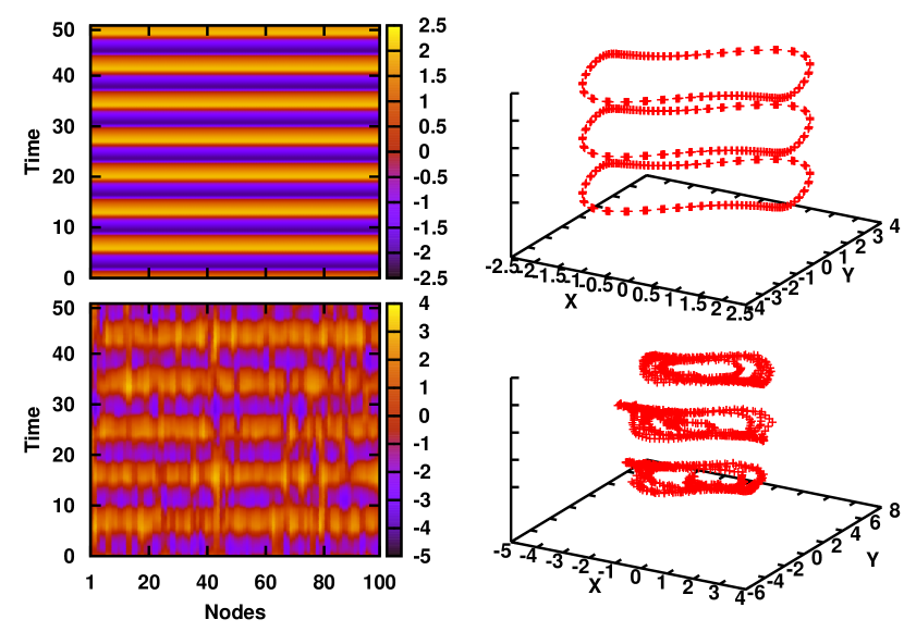
Figure 1: Evolution of $x_{i}(t)$ of all the oscillators ($i=1,\dots 100$), after a transient time of $15000$ (left), and the limit cycles of three representative oscillators stacked one above the other (right), for network rewiring period $r$ equal to $0.01$ (top row) and $0.1$ (bottom row). Here coupling strength $\varepsilon=0.6$ (which is significantly greater than $\varepsilon_{c}$) and the fraction of random links $p$ is $0.8$. Blow-up is prevented in both the cases, but faster rewiring leads to a synchronized state (top row) whereas slower rewiring leads to de-synchronization and distortion in the shape of the limit cycles (right panel, bottom row). Note that for this value of coupling strength, regular nearest neighbour coupling ($p=0$) would lead to a blow-up.

We show our results for representative values of $p$ and $r$ in Figure 1. Notice that the coupling strengths shown in the figure are greater than the critical value $\epsilon_{c}$, i.e. for these coupling strengths the limit cycles grow explosively for regular nearest neighbour coupling. However, it is clearly evident from the figure that the blow-up has been tamed when some fraction of the regular links are replaced by random links (i.e $p>0$). Namely, for sufficiently random networks, all oscillators remain confined in a bounded region of phase space.

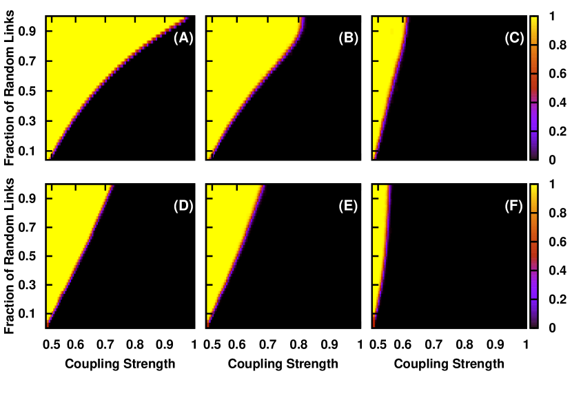
Figure 2: Transition between bounded and unbounded dynamics in a system of $100$ coupled oscillators, as reflected in the variation of the boundedness order parameter $Z_{bound}$ (see text) with increasing coupling strength $\varepsilon$ and fraction of random links $p$, for directed networks with network switching time period $r$ equal to (A) $0.01$, (B) $0.1$ and (C) $1$, and for undirected networks with $r$ equal to (D) $0.01$, (E) $0.1$ and (F) $1$.

In order to characterize the bounded-unbounded transitions quantitatively, we introduce a “boundedness order parameter”, $Z_{bound}$, which is given simply as the fraction of initial conditions for which the dynamics remained bounded. Thus $Z_{bound}$ gives the probability of successful prevention of blow-ups. Fig. 2 displays this quantity over a range of $p$ and $\varepsilon$. It is evident from Fig. 2, that for fraction of random links $p$ greater than a critical value, we always get a bounded state.

The fraction of random links necessary to obtain bounded dynamics with probability close to $1$ depends on the network switching time period $r$ and coupling strength $\varepsilon$ as indicated in Fig. 2. In general, for fast switching links, namely small $r$, the critical number of random links needed to suppress a blow-up is small. For very slow network changes however, one may not be able to quell explosive growth even with a large fraction of random links. So it is clear that rapidly changing links is the key to controlling the dynamics more efficiently.

Further, we studied the case of undirected networks (where $J$ in Eqn. 1 is a symmetric matrix). Qualitatively, similar results are obtained, though with reduced range for blow-up control (see lower panel of Fig. 2).

Now, in order to broadly rationalize this behavior we consider the dynamics of an individual oscillator in the system as a sum of the nodal dynamics and the coupling contributions of the form $c_{1}(t)$ and $c_{2}(t)$, whose strength is given by coupling constant $\epsilon$.

$$\dot{x} = y+\epsilon c_{1}(t)$$

$$\dot{y} = -\mu(x^{2}-1)y-x+\epsilon c_{2}(t)$$ (4)

When $c_{1}=0$ and $c_{2}=0$, the equations reduce to a single Van der-Pol oscillator, with a stable limit cycle and an unstable spiral repellor at the origin ($x^{*}=0,y^{*}=0$). When $c_{1}\neq 0$, $c_{2}\neq 0$, the effective dynamics of each oscillator in the network (Eqn. 4) can be seen as an oscillator with fluctuating parameters $c_{1}$ and $c_{2}$ fuzzy . Note that when $c_{1}\neq 0$ one obtains the fixed point solutions to be:

$$x^{*} = \frac{1\pm\sqrt{1-4\mu\epsilon^{2}c_{1}(c_{2}-\mu c_{1})}}{2\epsilon\mu c_{1}}$$

$$y^{*} = -\epsilon c_{1}$$ (5)

This implies that we get two fixed point solutions for each oscillator in the coupled system. For very weak coupling ($\varepsilon\rightarrow 0$) the additional fixed point sits at infinity. As coupling strength increases this fixed point migrates towards the limit cycle, and at some critical coupling strength collides with it, undergoing a saddle node bifurcation. This global bifurcation leads to the destruction of the attracting limit cycle and consequent blow-up. Now for noisy parameters $c_{1}$ and $c_{2}$, such a collision leading to an annihilation of the limit cycle occurs for sufficiently large fluctuations in $c_{1}$ and $c_{2}$ fuzzy . Since the magnitude of fluctuations is governed directly by coupling strength, this implies that blow-ups may occur for sufficiently large $\varepsilon$.

In this scenario, the underlying mechanism that allows the control of blow-up for random links is the following: when the links are changed rapidly (i.e. $r$ is small), to first approximation, the terms $c_{1}(t)$ and $c_{2}(t)$ in Eqn. 4, averages to zero, as it is a sum of uncorrelated random inputs. This effectively yields the condition for a single Van der Pol oscillator, namely no blow-up. Alternately, one can argue that for rapid random switching of coupling connections, the deviations from the single oscillator dynamics, is essentially a sum of uncorrelated contributions, which to first approximation average out to zero.

Synchronization of the Bounded State

Returning to the space-time plots displayed in Fig.1 we notice an additional feature. In the figure two cases with different network rewiring time periods are shown: a fast rewiring case and the slow network change scenario. While there is no blow-up in either case, the emergent bounded state is different for networks rewiring at different rates. When the underlying network changes rapidly one obtains a synchronized state barahona -hong , as evident in the representative example in the upper panel of Fig. 1. However, slow network changes yield bounded dynamics that is not synchronized, as typically seen in the representative example in the lower panel of Fig. 1.

So we will now investigate, in detail, the synchronization properties of the system. Specifically we attempt to answer the following question: when random coupling prevents a blow-up, does it yield a state that is synchronized, or not? In order to quantify the degree of synchronization in the network, we compute an average error function as the synchronization order parameter, defined as the mean square deviation of the instantaneous states of the nodes:

$$Z=\frac{1}{N}\sum_{i=1}^{N}\{[x_{i}(t)-\langle x(t)\rangle]^{2}\},$$ (6)

where, $\langle x(t)\rangle$ is the space average at time $t$. This quantity $Z$, averaged over time $n$ and over different initial conditions, is denoted as $Z_{sync}$. When $Z_{sync}=0$, we have complete synchronization.

Note that the time needed to reach synchronization is not simply monotonic with respect to fraction of random links intermediatep . Instead we observe a region, at intermediate values of $p$, where the transience becomes large. This kind of behavior is reminiscent of the long persistence of transience arising for intermediate values of network connectivity transience . So, in our calculation of the relevant order parameters we have left sufficiently long transience ($\sim 15000$).

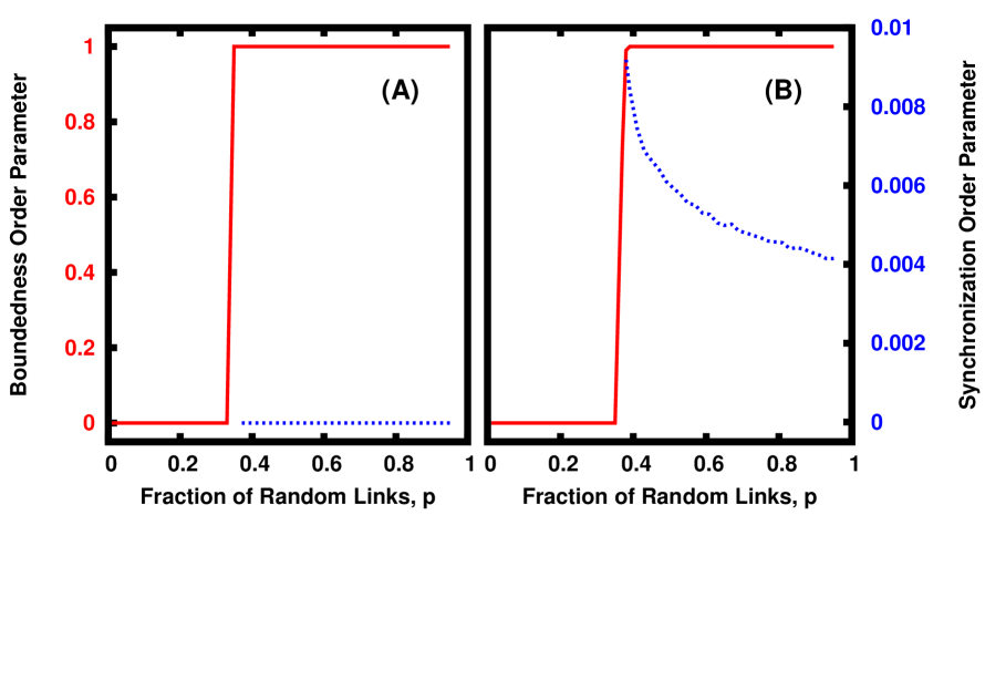
Figure 3: Variation of the Boundedness Order Parameter $Z_{bound}$ (solid red curve) and the Synchronization Order Parameter $Z_{sync}$ (dotted blue curve), averaged over $100$ initial conditions, with respect to fraction of random links $p$ for network rewiring time period (A) $r=0.01$ and (B) $r=0.1$. Here system size $N=100$ and coupling strength $\epsilon=0.6$, which is significantly greater than $\varepsilon_{c}$.

It is evident from Fig. 3 that in this particular system, for $p=0$, namely a regular ring, there is no synchronization, even at the largest allowed coupling strengths before blow-up, i.e. no $\epsilon<\epsilon_{c}$ yields a synchronized state. However for networks that change connections fast (i.e. $r$ is sufficiently small) the bounded state that arises after random rewiring is also synchronized. This is evident, quantitatively, through the vanishingly small synchronization error ($Z_{sync}\sim 0$) in networks where blow-ups have been completely suppressed (i.e. $Z_{bound}=1$). On the other hand, for slowly changing networks, the synchronization error is significant, even when the dynamics is bounded, i.e. $Z_{sync}$ is not close to zero even when $Z_{bound}=1$, as evident in Fig. 3b. So infrequent network changes have led to a state which is bounded but not synchronized, i.e. slowly switching random links are effective in reigning in the unbounded dynamics, but they do not manage to produce synchronization.

This relaxation oscillator network then yields three kinds of dynamical states: (i) bounded synchronized motion; (ii) bounded un-synchronized dynamics; and (iii) unbounded dynamics. The nature of the dynamics depends on the interplay of the coupling strength $\varepsilon$, rewiring probability $p$ and network switching time $r$.

Probabilistic Switching of Links

Now, periodic switching of links occurs in situations where the connections are determined by a global external periodic influence. However this is not always the most realistic scenario, as the interaction patterns may not change periodically in time. In such cases we must consider a probabilistic model of link switching, such as in Vazquez2010_1 ; Vazquez2010_2 . So in this subsection we study such randomly switched networks in order to determine if the ability to tame explosive growth is robust to the manner in which the links change. Namely, we verify the generality of our observations above by investigating the dynamics on a network whose underlying links switch randomly and asynchronously in time.

Specifically now, at each instant of time, a link has a probability $p_{r}$ of being rewired (the “link rewiring probability”). So when $p_{r}$ is higher the links are switched around more often. Note that as before, when a node rewires, it links to its nearest neighbours with probability $1-p$ and to some random site with probability $p$.

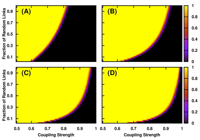
Figure 4: Transition between bounded and unbounded dynamics in a system of $100$ coupled oscillators with probabilistically switched links, as reflected in the variation of the boundedness order parameter $Z_{bound}$ (see text) with increasing coupling strength $\varepsilon$ and fraction of random links $p$. The link switching probability $p_{r}$ is: (A) $0.1$, (B) $0.3$ (C) $0.6$ and (D) $0.9$.

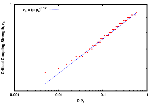
Figure 5: Variation of the critical coupling strength at which blow-up occurs, $\varepsilon_{c}$, with respect to the product of the link rewiring probability $p_{r}$ and fraction of random links $p$. The points are data from a wide range of $p$ and $p_{r}$, and they collapse to the scaling form shown by the line: $\epsilon_{c}\sim(p\ p_{r})^{\beta}$ with $\beta=0.12$.

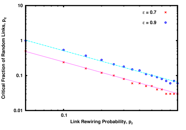
Figure 6: Variation of the minimum fraction of random links necessary to prevent blow-ups vs link rewiring probability $p_{r}$, at coupling strengths $\epsilon=0.7$ (red) and $0.9$ (blue). The straight lines show the fit to the scaling form: $p_{c}\sim p_{r}^{-1}$

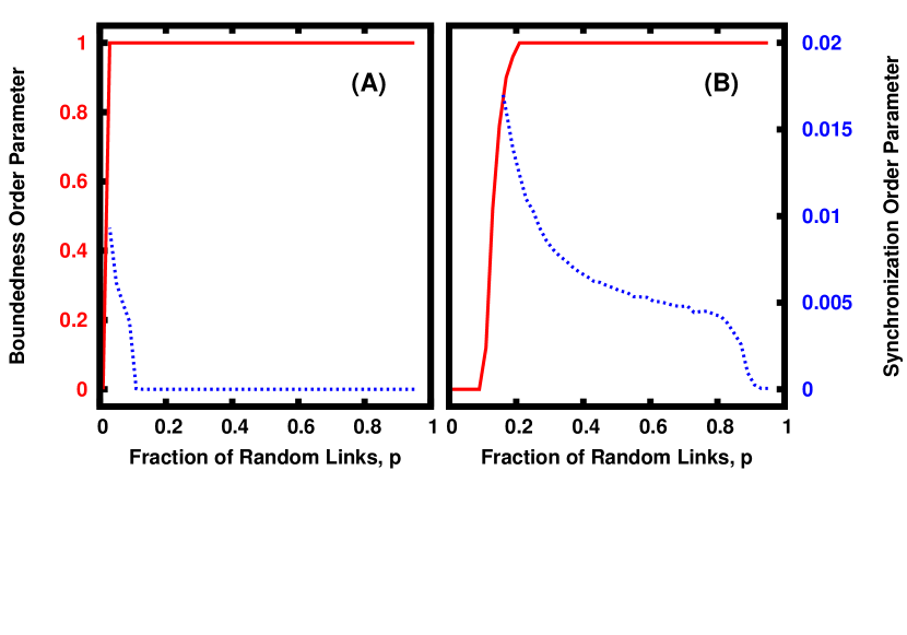
Figure 7: Variation of the Boundedness Order Parameter $Z_{bound}$ (solid red curve) and the Synchronization Order Parameter $Z_{sync}$ (dotted blue curve), averaged over $100$ initial conditions, with respect to fraction of random links $p$ for link rewiring probability (A) $p_{r}=0.9$ and (B) $p_{r}=0.1$. Here system size $N=100$ and coupling strength $\epsilon=0.6$, which is significantly greater than $\varepsilon_{c}$.

The results are displayed in Figs. 4-7. As in the case of periodically changing networks, here too random links manage to control the explosive growth in the system, for sufficiently large fraction of random links. Also, clearly, when the probability of rewiring the links is larger, namely when the network changes more often, the critical coupling strength at which blow-up occurs is pushed back, yielding a larger region of bounded dynamics.

Further, we observe that for networks that change connections fast (i.e. when $p_{r}$ is large) the bounded state that arises after random rewiring is also synchronized, as evident quantitatively through the vanishingly small synchronization error in these networks (cf. Fig. 7a). However, for slowly changing networks (i.e. when $p_{r}$ is small), the synchronization error is quite significant, even when the dynamics is bounded (cf. Fig. 7b), namely, slowly changing links yield a state that is bounded but not synchronized.

Inspecting further the interplay of the fraction of random links $p$, and the link rewiring probability $p_{r}$, reveals some interesting scaling relations. Notice first that the critical coupling strength $\epsilon_{c}$ beyond which blow-ups occur, scales with the link rewiring probability $p_{r}$ and fraction of random link $p$ as:

$$\epsilon_{c}\ \ \sim\ \ (p\ p_{r})^{\beta}$$

with $\beta\sim 0.12$. This is clearly evident, quantitatively, in the data collapse displayed in Fig. 5. This scaling relation implies that as the connections change more frequently, and there is larger fraction of random links in the connectivity matrix, the range over which bounded dynamics is obtained becomes larger. Also notice that the effective quantity that is relevant in the scaling relation is the product of $p$ and $p_{r}$, i.e. $p$ and $p_{r}$ may vary, but the emergent phenomena is the same if their product remains the same.

Further calculating the minimum fraction of random links $p_{c}$ necessary to prevent blow-ups, for a fixed coupling strength, at different link rewiring probabilities $p_{r}$ (cf. Fig. 6) reveals that

$$p_{c}\ \ \sim\ \ p_{r}^{-1}$$

Namely, when the system has large spatial randomness, infrequent changes of links manages to suppress blow-ups, while in a system with few spatially random connections, the links need to change more often in order to effect containment of blow-ups. This again implies (as did the scaling form in Fig. 5) that blow-ups can actually be tamed at quite small link rewiring probabilities and in networks with small fraction of random links, underscoring the broader relevance of our observations.

Generality of our central result

Finally, in order to further gauge the generality of the above findings, we investigated different coupling forms and local dynamics. For instance, we studied some other forms of nonlinear coupling, such as:

$${\dot{x}}_{i} = f(x_{i}+\frac{\varepsilon}{2}[x_{i-1}+x_{i+1}-2x_{i}],y_{i}+\frac{\varepsilon}{2}[y_{i-1}+y_{i+1}-2y_{i}])$$

$${\dot{y}}_{i} = g(x_{i}+\frac{\varepsilon}{2}[x_{i-1}+x_{i+1}-2x_{i}],y_{i}+\frac{\varepsilon}{2}[y_{i-1}+y_{i+1}-2y_{i}])$$ (7)

and

$${\dot{x}}_{i} = f(x_{i},y_{i})+\frac{\varepsilon}{2}[x_{i-1}^{2}+x_{i+1}^{2}-2x_{i}^{2}])$$

$${\dot{y}}_{i} = g(x_{i},y_{i})+\frac{\varepsilon}{2}[y_{i-1}^{2}+y_{i+1}^{2}-2y_{i}^{2}])$$ (8)

We also investigated the case where only one dynamical equation is coupled:

$${\dot{x}}_{i} = f(x_{i},y_{i})+\frac{\varepsilon}{2}[f(x_{i-1},y_{i-1})+f(x_{i+1},y_{i+1})-2f(x_{i},y_{i})]$$

$${\dot{y}}_{i} = g(x_{i},y_{i})$$ (9)

Since $f(x,y)=y$ in the Van der Pol oscillator, this coupling is similar to linear coupling of conjugate or dissimilar variables. The stability of the synchronized state in this system is amenable to analysis through the master stability function formalism msf and shows the following: the maximum Floquet multiplier remains positive for at least one eigen-mode, for all coupling strengths, implying that the synchronized solution is not stable under this form of coupling in regular networks.

Now, simulating all these different coupling forms above (Eqns. 7, 8 and 9), with some fraction of links randomized, displayed the same qualitative phenomena: After a certain critical coupling strength we encountered a blow-up in a regular ring of these oscillators, with the blow-ups occurring very early in some systems (e.g. $\epsilon_{c}<0.1$ in Eqn. 8). However, as observed in the earlier systems, dynamically randomizing the links in the network suppressed this explosive growth yielding bounded dynamics over a larger range of coupling strengths. Note that the range of the bounded region depends on the specifics of the coupling form and the local dynamics, as well as the fraction and frequency of change of the random links.

Lastly, we have also investigated the global behaviour of the system under different nodal dynamics. For instance, we investigated collections of nonlinearly coupled Stuart-Landau oscillators, where the local dynamics was given by:

$$\dot{z}=(1+i\omega-|z|^{2})z$$ (10)

where $\omega$ is the frequency, and $z(t)=x(t)+iy(t)$.

We also studied nonlinearly coupled networks of FitzHugh-Nagumo oscillators, modelling neuronal populations, described by the local dynamics fn1 ; fn2 :

$$\dot{x} = x-x^{3}/3-y+I$$

$$\dot{y} = \varPhi(x+a-by)$$ (11)

where x is the membrane potential, y is the recovery variable and I is the magnitude of stimulus current.

Further, we have explored the heterogeneous case where the nonlinearity parameter $\mu$ is distributed over a range of positive values for the local Van der Pol oscillators.

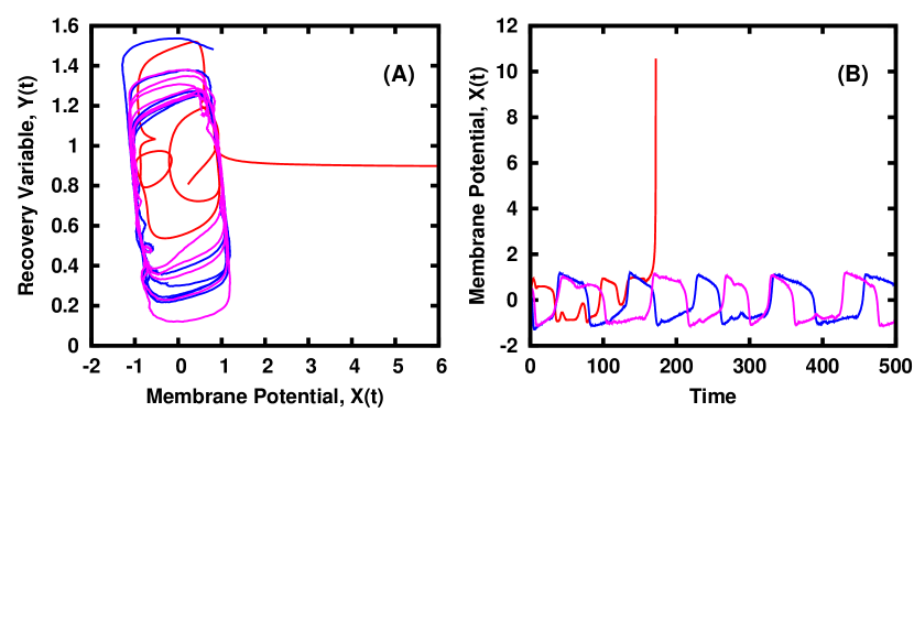
Figure 8: Phase portrait(left) and Time evolution of the membrane potential (right) for three representative FitzHugh-Nagumo model neurons in the network given by Eqn. 11, with fraction of random links $p=0.5$, time period of changing the links $r=0.01$, and coupling strength $\epsilon=0.54$ (cyan and blue curves). The case of a static regular network, exhibiting blow-up, is shown alongside as well (red curve). Note that the bounded orbits obtained under dynamic random links are not synchronized (cyan and blue curves).

Our extensive numerical simulations showed qualitatively similar behaviour for all of the above systems (see Fig. 8 for representative examples). This strongly suggests that the phenomenon of prevention of blow-ups through dynamic random links is quite general.

Conclusions

In summary, we have studied the dynamics of a collection of relaxation oscillators, under varying coupling topologies, ranging from a regular ring to a random network. We find that the system blows up under regular ring topology, for sufficiently strong coupling strength. However, when some fraction of the links are randomized dynamically, this blow-up is suppressed and the system remains bounded. So our results suggest an underlying mechanism by which complex systems can avoid a catastrophic blow-up. Further, from the stand point of potential applications, our observations indicate a method to control and prevent blow-ups in coupled oscillators that are commonplace in a variety of engineered systems.

Methods

We first present the method for changing the connectivity of the network.

Algorithm for Periodically Switching Networks:

1. We start with a $1$ dimensional ring, with $N$ nodes, where $N$ is the system size. Each node $i$ ($i=1,\dots N$) has $2$ links. In the network, a fraction $p$ of the links are to random nodes in the ring, and fraction $(1-p)$ are to nearest neighbours. So this network corresponds to a standard small world network Watts with degree $2$, with fraction of random links given by $p$.

2. After time $r$, change the $2$ existing connections for all nodes $i$. The new links are chosen such that, again, with probability $p$ they go to random neighbours, and with probability $(1-p)$ they are to nearest neighbours. So the changed network is also a standard small world network with degree $2$, with fraction of random links given by $p$.

3. Repeat step 2 again after every $r$ time steps.

So, while the fraction of random links is always $p$, the connectivity matrix of the system changes every $r$ steps. That is, $r$ is the network rewiring period.

Algorithm for Stochastically Switching Networks:

1. Again start with a $1$ dimensional ring, with $N$ nodes, where each node $i$ ($i=1,\dots N$) has $2$ links, and a fraction $p$ of the links are to random nodes, and fraction $(1-p)$ are to nearest neighbours.

2. Now at every instant of time, a node $i$ has probability $p_{r}$ to change its links. That is, $p_{r}$ gives the link rewiring probability of each individual node.

3. If the $2$ links of a certain node are changing, the new links are chosen such that, again, with probability $p$ they connect to random neighbours, and with probability $(1-p)$ they connect to nearest neighbours.

So in the above algorithm, the nodes change their links independently and stochastically, with probability $p_{r}$. That is, at any given time, fraction $p_{r}$ of the links change on an average, and $(1-p_{r})$ retain their existing links. The probability of the new links being random or regular is determined by $p$, as in the first algorithm (and as in the standard small-world scenario.)

Please note that in the first algorithm $r$ is the time period of link changes which occur globally throughout the network, while in the second algorithm the change occurs at the local level with probability $p_{r}$.

Our simulations show, that these two very different ways of varying the network, both yield the same qualitative phenomena: namely changing links helps to suppress blow-ups in the system.

Method for simulating the dynamics of the system: We solved the $2N$ coupled non-linear ordinary differential equations (ODE), given for instance by Eqns. 3, 7, 8, 9, by integrating the ODEs with the fourth order Runge-Kutta algorithm. We have checked that the results are qualitatively same over a large range of step sizes ($\sim 10^{-3}$ to $10^{-7}$), in order to rule out artefacts arising from the stiffness problem in such differential equations.

Using the above, we obtained the shapes and sizes of the limit cycles arising in this network under varying fraction of random links $p$ ($0\leq p\leq 1$) and a large range of network switching time periods $r$ ($0.01\leq r\leq 1$), for system sizes ranging from $N=10$ to $N=10^{3}$.

System Parameters : In the system given by Eqns. 2 and 3, we have investigated a range of nonlinearity parameters $\mu$, and we present the representative case of $\mu=1.5$ in the examples displayed in this paper. In the system given by Eqn. 11, parameters $\varPhi,a,b$ are taken to be $0.08,0.7,0.8$ respectively, in our simulations.

Acknowledgements

AC and VK acknowledge research fellowship from CSIR, India.

Author contributions

SS conceived the problem, and AC and VK performed all the numerical simulations. SS, AC and VK discussed the results and wrote the manuscript together.

The authors declare no competing financial interests.

References

- (1) Crutchfield, J., Kaneko, K. in Directions In Chaos, [Hao, B. L.(ed.)] (World Scientific, Singapore, 1987).
- (2) Wiesenfeld, K., Colet, P., Strogatz, S.H. Synchronization transitions in a disordered Josephson series array. Phys. Rev. Lett. 76, 404 (1996)
- (3) Perez, G., Pando-Lambruschini, C., Sinha, S., Cerdeira, H.A. Nonstatistical behavior of coupled optical systems. Phys. Rev. A 45, 5469(1992)
- (4) Zanette, D.H., Mikhailov, A.S. Condensation in globally coupled populations of chaotic dynamical systems. Phys. Rev. E 57, 276 (1998)
- (5) Wang, W., Kiss, I.Z., Hudson, J.L. Experiments on arrays of globally coupled chaotic electrochemical oscillators: Synchronization and clustering. Chaos 10, 248 (2000)
- (6) Barrow, J.D., The Infinite Book: A Short Guide To The Boundless, Timeless And Endless (Vintage, 2005).
- (7) Watts, D.J., Strogatz, S.H. Collective dynamics of âsmall-worldânetworks. Nature 393, 440 (1998).
- (8) Pecora, L.M., Carroll, T.L. Master stability functions for synchronized coupled systems. Phys. Rev. Lett. 80, 2109 (1998).
- (9) Van der Pol, B. On ârelaxation-oscillationsâ. The London, Edinburgh, and Dublin Philosophical Magazine and Journal of Science 2(11), 978-992 (1926)
- (10) Van der Pol, B., Van der Mark, J. Frequency demultiplication. Nature 120, 363-364 (1927).
- (11) Van der Pol, B., Van der Mark, J. The heartbeat considered as a relaxation oscillation, and an electrical model of the heart. The London, Edinburgh, and Dublin Philosophical Magazine and Journal of Science 6(38), 763-775 (1928)
- (12) FitzHugh, R. Impulses and physiological states in theoretical models of nerve membrane. Biophysical Journal 1(6), 445-466 (1961)
- (13) Nagumo, J., Arimoto, S., Yoshizawa, S. An active pulse transmission line simulating nerve axon. Proceedings of the Institute of Radio Engineers 50, 2061-2070 (1962)
- (14) Cartwright, J.H., Eguiluz, V.M., Hernandez-Garcia, E. & Piro,O. Dynamics of elastic excitable media. Internat. J. Bifur. Chaos Appl. Sci. Engrg. 9, 2197â2202 (1999).
- (15) Prasad, A., Dhamala, M., Adhikari, B.M., Ramaswamy, R. Amplitude death in nonlinear oscillators with nonlinear coupling. Phys. Rev. E 81, 027201 (2010).
- (16) Fitzgibbon, W.E., Walker, H.F., Nonlinear diffusion (Pitman, 1977).
- (17) Friston, K.J. Book Review: Brain Function, Nonlinear Coupling, and Neuronal Transients The Neuroscientist 7, 406-418 (2001)
- (18) Chen, C-C. et al, Nonlinear Coupling in the Human Motor System . J. of Neurosci. 30, 8393 (2010).
- (19) Muller-Stoffels, M., Wackerbauer, R. Regular network model for the sea ice-albedo feedback in the Arctic. Chaos 21, 013111 (2011).
- (20) Pastor, I., Perez-Garcia, V.M., Encinas, F., Guerra, J.M. Ordered and chaotic behavior of two coupled van der Pol oscillators. Phys. Rev. E 48, 171â182 (1993).
- (21) Sinha, S. Random coupling of chaotic maps leads to spatiotemporal synchronization. Phys. Rev. E 66, 016209 (2002)
- (22) Mondal, A., Sinha, S., Kurths, J. Rapidly switched random links enhance spatiotemporal regularity. Phys. Rev. E 78, 066209 (2008).
- (23) Varela, F., Lachaux, J.P., Rodriguez, E., Martinerie, J. The brainweb: phase synchronization and large-scale integration. Nat. Rev. Neurosci. 2, 229 (2001)
- (24) Brezina, V., Orekhova, I.V., Weiss, K.R. The neuromuscular transform: the dynamic, nonlinear link between motor neuron firing patterns and muscle contraction in rhythmic behaviors. J Neurophysiol. 83, 207 (2000).
- (25) Von der Malsburg, C. Handbook of Brain Theory and Neural Networks,[Dynamic Link Architecture, p.365] (MIT Press, 2002).
- (26) Sturis, J., Brøns, M. Local and global bifurcations at infinity in models of glycolytic oscillations. Journal of Mathematical Biology 36(2), 119â132 (1997)
- (27) Abraham, R.H., Bruce Stewart, H. A chaotic blue sky catastrophe in forced relaxation oscillations. Physica D 21, 394-400 (1986).
- (28) Hong, L., Sun, J.Q. A fuzzy blue sky catastrophe. Nonlinear Dynamics 55, 261-267 (2009).
- (29) McCann, K., Yodzis, P. Nonlinear dynamics and population disappearances. The American Naturalist 144, 873 (1994)
- (30) Ghosh, D., Banerjee, S., Chowdhury, A.R. Synchronization between variable time-delayed systems and cryptography. Euro. Phys. Letts. 80, 30006 (2007)
- (31) Barahona, M., Pecora, L.M. Synchronization in small-world systems. Phys. Rev. Lett. 89, 054101 (2002)
- (32) Matthews, P.C., Mirollo, R.E., Strogatz, S.H. Dynamics of a large system of coupled nonlinear oscillators. Physica D 52, 293 (1991)
- (33) Hong, H., Choi, M.Y., Kim, B.J. Synchronization on small-world networks. Phys. Rev. E 65, 026139 (2002)
- (34) Poria, S., Shrimali, M.D., Sinha, S. Enhancement of spatiotemporal regularity in an optimal window of random coupling. Phys. Rev. E 78, 035201 (2008).
- (35) Zumdieck, A., Timme, M., Geisel, T., and Wolf, F. Long chaotic transients in complex networks. Phys. Rev. Lett. 93, 244103 (2004)
- (36) Vazquez, F., Zanette, D.H. Epidemics and chaotic synchronization in recombining monogamous populations. Physica D 239, 1922-1928 (2010)
- (37) Zanette, D.H., Gusmán, S.R. Infection spreading in a population with evolving contacts. J. Biol. Phys. 34, 135 (2008)