The theory of the double preparation: discerned and indiscerned particles

Abstract

In this paper we propose a deterministic and realistic quantum mechanics interpretation which may correspond to Louis de Broglie’s "double solution theory". Louis de Broglie considers two solutions to the Schrödinger equation, a singular and physical wave u representing the particle (soliton wave) and a regular wave representing probability (statistical wave). We return to the idea of two solutions, but in the form of an interpretation of the wave function based on two different preparations of the quantum system. We demonstrate the necessity of this double interpretation when the particles are subjected to a semi-classical field by studying the convergence of the Schrödinger equation when the Planck constant tends to 0. For this convergence, we reexamine not only the foundations of quantum mechanics but also those of classical mechanics, and in particular two important paradox of classical mechanics: the interpretation of the principle of least action and the the Gibbs paradox. We find two very different convergences which depend on the preparation of the quantum particles: particles called indiscerned (prepared in the same way and whose initial density is regular, such as atomic beams) and particles called discerned (whose density is singular, such as coherent states). These results are based on the Minplus analysis, a new branch of mathematics that we have developed following Maslov, and on the Minplus path integral which is the analog in classical mechanics of the Feynman path integral in quantum mechanics. The indiscerned (or discerned) quantum particles converge to indiscerned (or discerned) classical particles and we deduce that the de Broglie-Bohm pilot wave is the correct interpretation for the indiscerned quantum particles (wave statistics) and the Schrödinger interpretation is the correct interpretation for discerned quantum particles (wave soliton). Finally, we show that this double interpretation can be extended to the non semi-classical case.

I Introduction

For Louis de Broglie, the correct interpretation of quantum mechanics was the "theory of the double solution" introduced in 1927 Broglie1927 and for which the pilot-wave was just a low-level product Broglie : I introduced as a ’double solution theory’ the idea that it was necessary to distinguish two different solutions but both linked to the wave equation, one that I called wave $u$ which was a real physical wave but not normalizable having a local anomaly defining the particle and represented by a singularity, the other one as the Schrödinger $\Psi$ wave, which is normalizable without singularities and being a probability representation.

Louis de Broglie distinguishes two solutions to the Schrödinger equation, a singular and physical wave $u$ representing the particle (soliton wave) and a regular wave $\Psi$ representing probability (statistical wave). But, de Broglie don’t have never find a consistent "double solution theory". We return to the idea of two solutions, but in the form of a double interpretation of the wave function based on different preparations of the quantum system. We demonstrate the necessity of this double interpretation when the particles are subjected to a semi-classical field by studying the convergence of the Schrödinger equation when the Planck constant tends to 0 Gondran2011 ; Gondran2012a . This convergence of quantum to classical mechanics poses three types of difficulty that seem insurmountable:

• a physical difficulty, because h is a constant and therefore its convergence to 0 is not physical;

• a conceptual difficulty: in quantum mechanics, particles are regarded as indistinguishable whereas they are considered to be distinguishable in classical mechanics;

• mathematical difficulties of convergence of equations.

The physical difficulty is the easiest to solve: it is only mathematically, not physically, that we decrease the Planck constant to 0; numerically we obtain the same results if we increase the mass $m$ of the particle to infinity.

The conceptual difficulty forces us into reexamining not only the foundations of quantum mechanics but also those of classical mechanics. It is necessary to understand and solve two important paradoxes of classical mechanics: the interpretation of the principle of least action where the "final causes" seem to be substituted for the "efficient causes"; the Gibbs paradox where the entropy calculation of a mixture of two identical gases by classical mechanics with distinguishable particles leads to an entropy twice as big as expected. We solve the conceptual difficulty by showing that it is natural to introduce the concepts of discerned and indiscerned particles both in classical mechanics and in quantum mechanics.

The mathematical difficulties will be greatly simplified by considering two types of initial conditions (discerned and indiscerned particles) which yield very different mathematical convergences. They are also simplified by the Minplus analysis Gondran_1996 ; GondranMinoux , a new branch of mathematics that we have developed following Maslov Maslov ; Maslov2 . The paper is organized as follows. In section II, we will show that the difficulties of interpretation of the principle of least action concerning the "final causes" come from the "Euler-Lagrange action" (or classical action) $S_{cl}(\textbf{x},t;\textbf{x}_{0})$, which links the initial position $\textbf{x}_{0}$ and its position x at time t and not from the "Hamilton-Jacobi action" $S(\textbf{x},t)$, which depends on an initial action $S_{0}(\textbf{x})$. These two actions are solutions to the same Hamilton-Jacobi equation, but with very different initial conditions: smooth conditions for the Hamilton-Jacobi action, singular conditions for the Euler-Lagrange action.

In section III, we show how Minplus analysis, a new branch of nonlinear mathematics, explains the difference between the Hamilton-Jacobi action and the Euler-Lagrange action. We obtain the equation between these two actions, which we call the Minplus path integral: it is the analog in classical mechanics of the Feynman path integral in quantum mechanics. We show that it is the key to understanding the principle of least action.

In section IV, we introduce in classical mechanics the concept of indiscerned particles through the statistical Hamilton-Jacobi equations. The discerned particles in classical mechanics correspond to a deterministic action $S(\textbf{x},t;\textbf{x}_{0},\textbf{v}_{0})$, which links a particle in initial position $\textbf{x}_{0}$ and initial velocity $\textbf{v}_{0}$ to its position x at time $t$ and verifies the deterministic Hamilton-Jacobi equations. And the Gibbs paradox is solved by the indiscerned particles in classical mechanics.

In section V, we study the convergence of quantum mechanics to classical mechanics when the Planck constant tends to 0 by considering two cases : the first corresponds to the convergence to an indiscerned classical particle, and the second corresponds to the convergence to a classical discerned particle. Gondran2011 ; Gondran2012a Based on these convergences, we propose a new interpretation of quantum mechanics, the "theory of the double preparation", a response that corresponds to Louis de Broglie’s "theory of the double solution".

In section VI, we generalize this interpretation when the semi-classical approximation is not valid. Following de Muynck Muynck , we show that it is possible to construct a deterministic field quantum theory that extends the previous double semi-classical interpretation to the non semi-classical case.

II The Euler-Lagrange and Hamilton-Jacobi actions

The intense debate on the interpretation of the wave function in quantum mechanics for eighty years has in fact left the debate on the interpretation of the action and the principle of least action in classical mechanics in the dark, since their introduction in 1744 by Pierre-Louis Moreau de Maupertuis Maupertuis1744 : "Nature, in the production of its effects, does so always by the simplest means […] the path it takes is the one by which the quantity of action is the least". Maupertuis understood that, under certain conditions, Newton’s equations are equivalent to the fact that a quantity, which he calls the action, is minimal. Indeed, one can verify that the trajectory realized in Nature is that which minimizes (or renders extremal) the action, which is a function depending on the different possible trajectories.

However, this principle has often been viewed as puzzling by many scholars, including Henri Poincaré, who was nonetheless one of its most intensive users Poincare : "The very enunciation of the principle of least action is objectionable. To move from one point to another, a material molecule, acted on by no force, but compelled to move on a surface, will take as its path the geodesic line, i.e., the shortest path. This molecule seems to know the point to which we want to take it, to foresee the time it will take to reach it by such a path, and then to know how to choose the most convenient path. The enunciation of the principle presents it to us, so to speak, as a living and free entity. It is clear that it would be better to replace it by a less objectionable enunciation, one in which, as philosophers would say, final effects do not seem to be substituted for acting causes."

We will show that the difficulties of interpretation of the principle of least action concerning the "final causes" or the "efficient causes" come from the existence of two different actions: the "Euler-Lagrange action" $S_{cl}(\textbf{x},t;\textbf{x}_{0})$ and the "Hamilton-Jacobi action" $S(\textbf{x},t)$.

Let us consider a system evolving from the position $\textbf{x}_{0}$ at initial time to the position x at time $t$ where the variable of control u(s) is the velocity:

$$\frac{d\textbf{x}\left(s\right)}{ds}=\mathbf{u}(s),\qquad\forall s\in\left[0,t\right]$$ (1)

$$\textbf{x}(0)=\mathbf{x}_{0},\qquad\textbf{x}(t)=\mathbf{x}.$$ (2)

If $L(\textbf{x},\dot{\textbf{x}},t)$ is the Lagrangian of the system, when the two positions $\textbf{x}_{0}$ and x are given, the Euler-Lagrange action $S_{cl}(\mathbf{x},t;\textbf{x}_{0})$ is the function defined by:

$$S_{cl}(\textbf{x},t;\mathbf{x}_{0})=\min_{\textbf{u}\left(s\right),0\leq s\leq t}\int_{0}^{t}L(\textbf{x}(s),\textbf{u}(s),s)ds,$$ (3)

where the minimum (or more generally an extremum) is taken on the controls $\mathbf{u}(s)$, $s\in$ $\left[0,t\right]$, with the state $\textbf{x}(s)$ given by equations (1) and (2). This is the principle of least action defined by Euler Euler1744 in 1744 and Lagrange Lagrange in 1755.

The solution $(\widetilde{\textbf{x}}(s),\widetilde{\textbf{u}}(s))$ of (3), if the Lagrangian $L(\textbf{x},\dot{\textbf{x}},t)$ is twice differentiable, satisfies the Euler-Lagrange equations on the interval $[0,t]$:

$$\frac{d}{ds}\frac{\partial L}{\partial\dot{\textbf{x}}}(\textbf{x}(s),\dot{\textbf{x}}(s),s)-\frac{\partial L}{\partial\textbf{x}}(\textbf{x}(s),\dot{\textbf{x}}(s),s)=0,\quad\forall s\in\left[0,t\right]$$ (4)

$$\textbf{x}(0)=\mathbf{x}_{0},~{}~{}~{}~{}\textbf{x}(t)=\mathbf{x}.$$ (5)

For a non-relativistic particle in a linear potential field with the Lagrangian $L(\mathbf{x},\mathbf{\dot{x}},t)=\frac{1}{2}m\mathbf{\dot{x}}^{2}+\textbf{K}.\textbf{x}$, equation (4) yields $\frac{d}{ds}(m\dot{\textbf{x}}(s))-\textbf{K}=0$. The trajectory minimizing the action is $\widetilde{\textbf{x}}(s)=\textbf{x}_{0}+\frac{s}{t}(\textbf{x}-\textbf{x}_{0})-\frac{\textbf{K}}{2m}ts+\frac{\textbf{K}}{2m}s^{2}$, and the Euler-Lagrange action is equal to

$$S_{cl}(\mathbf{x},t;\textbf{x}_{0})=m\frac{(\textbf{x}-\textbf{x}_{0})^{2}}{2t}+\frac{K.(\textbf{x}+\textbf{x}_{0})}{2}t-\frac{K^{2}}{24m}t^{3}.$$ (6)

Figure 1 shows different trajectories going from $x_{0}$ at time $t=0$ to $x$ at final time $t$. The parabolic trajectory $\widetilde{x}(s)$ corresponds to this which realizes the minimum in the equation (3).

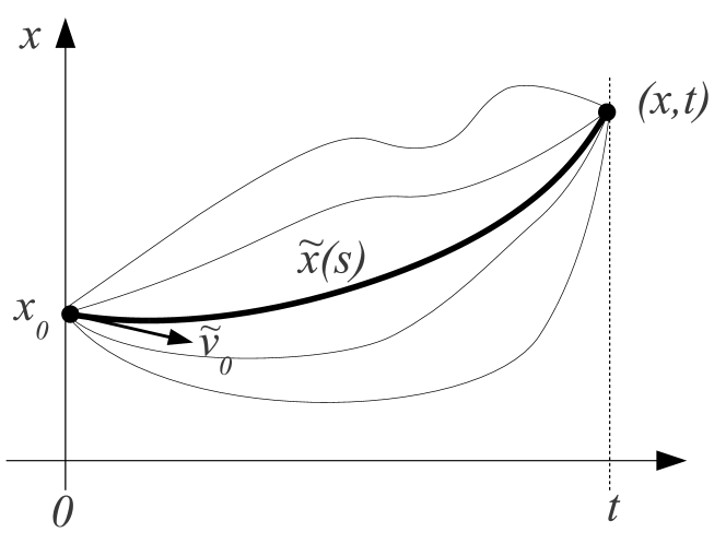
Figure 1: Different trajectories $x(s)$ ($0\leq s\leq t$) between $(x_{0},0)$ and $(x,t)$ and the optimal trajectory $\widetilde{x}(s)$ with $\widetilde{\textbf{v}}_{0}=\frac{\textbf{x}-\textbf{x}_{0}}{t}-\frac{Kt}{2m}$.

Equation (3) seems to show that, among the trajectories which can reach ($\textbf{x},t$) from the initial position $\textbf{x}_{0}$, the principle of least action allows to choose the velocity at each time. In reality, the principle of least action used in equation (3) does not choose the velocity at each time $s$ between $0$ and $t$, but only when it arrives at x at time $t$. The knowledge of the velocity at each time $s$ ($0\leq s\leq t$) requires the resolution of the Euler-Lagrange equations (4,5) on the whole trajectory. In the case of a non-relativistic particle in a linear potential field, the velocity at time $s$ ($0\leq s\leq t$) is $\widetilde{\textbf{v}}(s)=\frac{\textbf{x}-\textbf{x}_{0}}{t}-\frac{Kt}{2m}+\frac{Ks}{m}$ with the initial velocity

$$\widetilde{\textbf{v}}_{0}=\frac{\textbf{x}-\textbf{x}_{0}}{t}-\frac{Kt}{2m}.$$ (7)

Then, $\widetilde{\textbf{v}}_{0}$ depends on the position x of the particle at the final time $t$. This dependence of the "final causes" is general. This is the Poincaré’s main criticism of the principle of least action: "This molecule seems to know the point to which we want to take it, to foresee the time it will take to reach it by such a path, and then to know how to choose the most convenient path."

One must conclude that, without knowing the initial velocity, the Euler-Lagrange action answers a problem posed by an observer, and not by Nature: "What would be the velocity of the particle at the initial time to arrive in x at time $t$?" The resolution of this problem implies that the observer solves the Euler-Lagrange equations (4,5) after the observation of x at time $t$. This is an a posteriori point of view.

But from 1830, Hamilton Hamilton proposes to consider the action $S$ as a function of the coordinates and of the time $S(\textbf{x},t)$. It is customary to call it Hamilton’s principal functionLandau ; Goldstein ; Butterfield . In the following, we refer to it as the Hamilton-Jacobi action. Indeed, for the Lagrangian $L(\mathbf{x},\mathbf{\dot{x}},t)=\frac{1}{2}m\mathbf{\dot{x}}^{2}-V(\textbf{x},t)$, this action satisfies the Hamilton-Jacobi equations:

$$\frac{\partial S}{\partial t}+\frac{1}{2m}(\triangledown S)^{2}+V(\textbf{x},t)=0$$ (8)

$$S(\textbf{x},0)=S_{0}(\textbf{x}).$$ (9)

The initial condition $S_{0}(\textbf{x})$ is essential to defining the general solution to the Hamilton-Jacobi equations (8,9) although it is ignored in the classical mechanics textbooks such as those of Landau Landau chap.7 § 47 and Goldstein Goldstein chap. 10. However, the initial condition $S_{0}(\textbf{x})$ is mathematically necessary to obtain the general solution to the Hamilton-Jacobi equations. Physically, it is the condition that describes the preparation of the particles. We will see that this initial condition is the key to understanding the principle of least action.

The main property of the Hamilton-Jacobi action is that the velocity of a non-relativistic classical particle is given for each point $\left(\mathbf{x,}t\right)$ by:

$$\mathbf{v}\left(\mathbf{x,}t\right)=\frac{\mathbf{\nabla}S\left(\mathbf{x,}t\right)}{m}.$$ (10)

In the general case where $S_{0}(\textbf{x})$ is a regular function, for example differentiable, equation (10) shows that the solution $S\left(\mathbf{x,}t\right)$ of the Hamilton-Jacobi equations yields the velocity field for each point ($\textbf{x},t$) from the velocity field $\frac{\nabla S_{0}(\textbf{x})}{m}$ at the initial time. In particular, if at the initial time, we know the initial position $\textbf{x}_{init}$ of a particle, its velocity at this time is equal to $\frac{\nabla S_{0}(\textbf{x}_{init})}{m}$. From the solution $S\left(\mathbf{x,}t\right)$ of the Hamilton-Jacobi equations, we deduce with (10) the trajectories of the particle. The Hamilton-Jacobi action $S\left(\mathbf{x,}t\right)$ is then a field which "pilots" the particle.

There is another solution to the Hamilton-Jacobi equation; it is the Euler-Lagrange action. Indeed, $S_{cl}(\textbf{x},t;\textbf{x}_{0})$ satisfies the Hamilton-Jacobi (8) with the initial condition

$$S(\textbf{x},0)=\{0~{}\text{ if }~{}\textbf{x}=\textbf{x}_{0},+\infty~{}\text{ if not}\}$$ (11)

which is a very singular function. Mathematical analysis will help us to interpret the solution to the Hamilton-Jacobi equations and the principle of least action.

III Minplus analysis and the Minplus path integral

There exists a new branch of mathematics, Minplus analysis, which studies nonlinear problems through a linear approach, cf. Maslov Maslov ; Maslov2 and Gondran Gondran_1996 ; GondranMinoux . The idea is to substitute the usual scalar product $\int_{X}f(x)g(x)dx$ with the Minplus scalar product:

$$(f,g)=\inf_{x\in X}\left\{f(x)+g(x)\right\}$$ (12)

In the scalar product we replace the field of the real number $(\mathbb{R},+,\times)$ with the algebraic structure Minplus $(\mathbb{R}\cup\{+\,\infty\},\min,+)$, i.e. the set of real numbers (with the element infinity $\{+\infty\}$) endowed with the operation Min (minimum of two reals), which remplaces the usual addition, and with the operation + (sum of two reals), which remplaces the usual multiplication. The element $\{+\,\infty\}$ corresponds to the neutral element for the operation Min, Min$(\{+\infty\},a)=a$ $\forall a\in\mathbb{R}$. This approach bears a close similarity to the theory of distributions for the nonlinear case; here, the operator is "linear" and continuous with respect to the Minplus structure, though nonlinear with respect to the classical structure $\left(\mathbb{R},+,\times\right)$. In this Minplus structure, the Hamilton-Jacobi equation is linear, because if $S_{1}(\textbf{x},t)$ and $S_{2}(\textbf{x},t)$ are solutions to (8), then $\min\{\lambda+S_{1}(\textbf{x},t),\mu+S_{2}(\textbf{x},t)\}$ is also a solution to the Hamilton-Jacobi equation (8).

The analog to the Dirac distribution $\delta(\textbf{x})$ in Minplus analysis is the nonlinear distribution $\delta_{\min}(\textbf{x})=\{0~{}\text{ if }~{}\textbf{x}=\textbf{0},+\infty~{}\text{ if not}\}$. With this nonlinear Dirac distribution, we can define elementary solutions as in classical distribution theory. In particular, we obtain:

The classical Euler-Lagrange action $S_{cl}(\textbf{x},t;\textbf{x}_{0})$ is the elementary solution to the Hamilton-Jacobi equations (8)(9) in the Minplus analysis with the initial condition

$$S(\textbf{x},0)=\delta_{\min}(\textbf{x}-\textbf{x}_{0})=\{0~{}\text{ if }~{}\textbf{x}=\textbf{x}_{0},~{}+\infty~{}\text{ if not}\}.$$ (13)

The Hamilton-Jacobi action $S(\textbf{x},t)$ is then given by the Minplus integral

$$S(\textbf{x},t)=\inf_{\textbf{x}_{0}}\{S_{0}(\textbf{x}_{0})+S_{cl}(\textbf{x},t;\textbf{x}_{0})\}.$$ (14)

that we call the Minplus path integral. It is an equation similar to the Hopf-Lax formulaLions ; Evans . This equation is in analogy with the solution to the heat transfer equation given by the classical integral:

$$S(x,t)=\int S_{0}(x_{0})\frac{1}{2\sqrt{\pi t}}e^{-\frac{\left(x-x_{0}\right)^{2}}{4t}}dx_{0},$$ (15)

which is the product of convolution of the initial condition $S_{0}(x)$ with the elementary solution to the heat transfer equation $e^{-\frac{x^{2}}{4t}}$.

This Minplus path integral yields a very simple relation between the Hamilton-Jacobi action, the general solution to the Hamilton-Jacobi equation, and the Euler-Lagrange actions, the elementary solutions to the Hamilton-Jacobi equation. We can also consider that the Minplus integral (14) for the action in classical mechanics is analogous to the Feynmann path integral for the wave function in quantum mechanics. Indeed, in the Feynman paths integral Feynman_1965 (p. 58), the wave function $\Psi(\textbf{x},t)$ at time $t$ is written as a function of the initial wave function $\Psi_{0}(\textbf{x})$:

$$\Psi(\textbf{x},t)=\int F(t,\hbar)\exp\left(\frac{i}{\hbar}S_{cl}(\textbf{x},t;\textbf{x}_{0}\right)\Psi_{0}(\textbf{x}_{0})d\textbf{x}_{0}$$ (16)

where $F(t,\hbar)$ is an independent function of x and of $\textbf{x}_{0}$.

For a particle in a linear potential $V(\textbf{x})=-\textbf{K}.\textbf{x}$ with the initial action $S_{0}(\textbf{x})=m\textbf{v}_{0}\cdot\textbf{x}$, we deduce from equation (14) that the Hamilton-Jacobi action is equal to $S\left(\mathbf{x},t\right)=m\textbf{v}_{0}\cdot\textbf{x}-\frac{1}{2}m\textbf{v}_{0}^{2}t+\textbf{K}.\textbf{x}t-\frac{1}{2}\textbf{K}.\textbf{v}_{0}t^{2}-\frac{\textbf{K}^{2}t^{3}}{6m}$.

Figure 2 shows the classical trajectories (parabols) going from different starting points $x^{i}_{0}$ at time $t=0$ to the point $x$ at final time $t$. The Hamilton-Jacobi action is compute with these trajectories in the Minplus path integral (14).

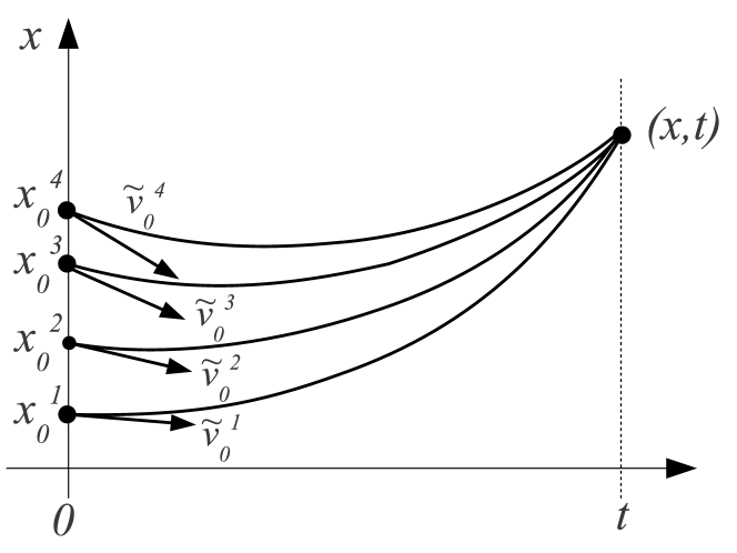
Figure 2: Classical trajectories $\widetilde{x}(s)$ ($0\leq s\leq t$) between the different initial positions $x^{i}_{0}$ and the position $x$ at time $t$. We obtain $\widetilde{\textbf{v}}^{i}_{0}=\frac{\textbf{x}-\textbf{x}^{i}_{0}}{t}-\frac{Kt}{2m}$.

Finally, we can write the Minplus paths integral as follows:

$$S(\mathbf{x},t)=\min_{\textbf{x}_{0};\mathbf{u}\left(s\right),0\leq s\leq t}\left\{S_{0}\left(\mathbf{x}_{0}\right)+\int_{0}^{t}L(\textbf{x}(s),\mathbf{u}(s),s)ds\right\}$$ (17)

where the minimum is taken on all initial positions $\textbf{x}_{0}$ and on the controls $\mathbf{u}(s)$, $s\in$ $\left[0,t\right]$, with the state $\textbf{x}(s)$ given by equations (1) and (2). This is possible because $S_{0}(\textbf{x}_{0})$ does not play a role in (17) for the minimization on $\textbf{u}(s)$.

Equation (17) seems to show that, among the trajectories which can reach ($\textbf{x},t$) from an unknown initial position and a known initial velocity field, Nature chooses the initial position and at each time the velocity that yields the minimum (or the extremum) of the Hamilton-Jacobi action.

Equations (10), (8) and (9) confirm this interpretation. They show that the Hamilton-Jacobi action $S(\mathbf{x},t)$ does not solve only a given problem with a single initial condition $\left(\mathbf{x}_{0},\frac{\mathbf{\nabla}S_{0}\left(\mathbf{x}_{0}\right)}{m}\right)$, but a set of problems with an infinity of initial conditions, all the pairs $\left(\mathbf{y},\frac{\mathbf{\nabla}S_{0}\left(\mathbf{y}\right)}{m}\right)$. It answers the following question: "If we know the action (or the velocity field) at the initial time, can we determine the action (or the velocity field) at each later time?" This problem is solved sequentially by the (local) evolution equation (8). This is an a priori point of view. It is the problem solved by Nature with the principle of least action.

For a particle in a linear potential $V(\textbf{x})=-\textbf{K}.\textbf{x}$ with the initial action $S_{0}(\textbf{x})=m\textbf{v}_{0}\cdot\textbf{x}$, the initial velocity field is constant, $\textbf{v}(\textbf{x},0)=\frac{\mathbf{\nabla}S_{0}\left(\mathbf{x}\right)}{m}=\textbf{v}_{0}$ and the velocity field at time $t$ is also constant, $\textbf{v}(\textbf{x},t)=\frac{\mathbf{\nabla}S\left(\mathbf{x},t\right)}{m}=\textbf{v}_{0}+\frac{\textbf{K}t}{m}$. Figure 3 shows these velocity fields.

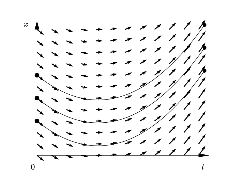
Figure 3: Velocity field that corresponds to the Hamilton-Jacobi action $S\left(\mathbf{x},t\right)=m\textbf{v}_{0}\cdot\textbf{x}-\frac{1}{2}m\textbf{v}_{0}^{2}t+\textbf{K}.\textbf{x}t-\frac{1}{2}\textbf{K}.\textbf{v}_{0}t^{2}-\frac{\textbf{K}^{2}t^{3}}{6m}$ ($\textbf{v}(\textbf{x},t)=\frac{\mathbf{\nabla}S\left(\mathbf{x},t\right)}{m}=\textbf{v}_{0}+\frac{\textbf{K}t}{m}$) and three trajectories of particles piloted by this field.

IV Discerned and indiscerned particles in classical mechanics

We show that the difficulties interpreting the action and the wave function result from the ambiguity in the definition of the conditions for the preparation of particles, which entails an ambiguity concerning the initial conditions. This ambiguity is related to the notion of indiscernibility which has never been well defined in the literature. It is responsible in particular for the Gibbs paradox: when calculating the entropy of a mixture of two identical gases in equilibrium, calculation by classical mechanics with distinguishable particles leads to an entropy twice as big as expected. If we replace these particles with indistinguishable particles, then the factor related to the indiscernibility yields the correct result.

In almost all textbooks on statistical mechanics, it is considered that this paradox stated by Willard Gibbs in 1889, was "solved" by quantum mechanics over thirty-five years later, thanks to the introduction of the indistinguishability postulate for identical quantum particles. Indeed, it was Einstein who, in 1924, introduced the indistinguishability of molecules of an ideal gas at the same time as the Bose-Einstein statistics. Nonetheless, as pointed out by Henri Bacry, "history might have followed a different path. Indeed, quite logically, we could have applied the principle of indiscernibility to save the Gibbs paradox. […] This principle can be added to the postulates of quantum mechanics as well as to those of classical mechanics". Bacry

This same observation has been made by a large number of other authors. In 1965 Landé Lande_1965 demonstrated that this indiscernability postulate of classical particles is sufficient and necessary in order to explain why entropy vanished. In 1977, Leinaas and Myrheim Leinaas_1976 used it for the foundation of their identical classical and quantum particles theory. Moreover, as noted by Greiner et al. Greiner_1999 , in addition to the Gibbs paradox, several cases where it is needed to consider indistinguishable particles in classical mechanics and distinguishable particles in quantum mechanics can be found: "Hence, the Gibbs factor $\frac{1}{N!}$ is indeed the correct recipe for avoiding the Gibbs paradox. From now on we will therefore always take into account the Gibbs correction factor for indistinguishable states when we count the microstates. However, we want to emphasize that this factor is no more than a recipe to avoid the contradictions of classical statistical mechanics. In the case of distinguishable objects (e.g., atoms which are localized at certain grid points), the Gibbs factor must not be added. In classical theory the particles remain distinguishable. We will meet this inconsistency more frequently in classical statistical mechanics." Greiner_1999 p.134

We propose an accurate definition of both discernability and indiscernability in classical mechanics and a way to avoid ambiguities and paradoxes. Here, we only consider the case of a single particle or a system of identical particles without interactions and prepared in the same way.

In classical mechanics, a particle is usually considered as a point and is described by its mass $m$, its charge if it has one, as well as its position $x_{0}$ and velocity $v_{0}$ at the initial instant. If the particle is subject to a potential field $V(x)$, we can deduce its path because its future evolution is given by Newton’s or Lorentz’s equations. This is why classical particles are considered distinguishable. We will show, however, that a classical particle can be either non-discerned or discerned depending on how it is prepared.

We now consider a particle within a stationary beam of classical identical particles such as electronic, atomic or molecular beams ($CO_{2}$ or $C_{60}$). At a very macroscopic level, one can consider a tennis ball canon. Let us note that there is an abuse of language when one talks about a classical particle. One should instead speak of a particle that is studied in the framework of classical mechanics.

For a particle of this beam, we do not know at the initial instant the exact position or the exact velocity, only the characteristics describing the beam, that is to say, an initial probability density $\rho_{0}\left(\mathbf{x}\right)$ and an initial velocity field $\mathbf{v}_{0}(\textbf{x})$ known through the initial action $S_{0}(\textbf{x})$ by the equation $\mathbf{v}_{0}(\textbf{x})=\frac{\nabla S_{0}(\textbf{x})}{m}$ where $m$ is the particle mass. This yields the following definition:

Definition 1 (Indiscerned prepared Particle)

- A classical particle is said to be indiscerned prepared when only the characteristics of the beam from which it comes (initial probability density $\rho_{0}\left(\textbf{x}\right)$ and initial action $S_{0}(\textbf{x})$) are defined at the initial time.

In contrast, we have:

Definition 2 (Discerned prepared Particle)

- A classical particle is said to be discerned prepared, if one knows, at the initial time, its position $\textbf{x}_{0}$ and velocity $\textbf{v}_{0}$.

The notion of indiscernibility that we introduced does not depend on the observer’s knowledge, but is related to the mode of preparation of the particle.

Let us consider $N$ indiscerned particles, that is to say $N$ identical particles prepared in the same way, each with the same initial density $\rho_{0}\left(\textbf{x}\right)$ and the same initial action $S_{0}(\textbf{x})$, subject to the same potential field $V(\textbf{x})$ and which will have independent behaviors. This is particularly the case of identical classical particles without mutual interaction and prepared the same way. It is also the case of identical classical particles such as electrons, prepared in the same way and which, although they may interact, will have independent behaviors if they are generated one by one in the system.

We called these particles indiscerned, and not indistinguishable, because if we knew their initial positions, their trajectories would be known.

The difference between discerned and indiscerned particles depends on the preparation style. A device prepares either discerned or indiscerned particles. By way of example a tennis ball machine randomly launches balls in different directions. Therefore it prepares some indiscerned particles; only the characteristics of the balls’ beams are known: probability of presence and velocity (action). A tennis player plunged into complete darkness that uses this machine knows only the presence probability of balls. However it is possible to discern indiscerned particles, if we knew their initial positions. This is what happens during the day: the tennis player is able to make successive measurements of the ball position by watching it. In this case, the player is able to plan the trajectory. It is important to note that without measurements, the balls remain indiscerned. In this specific case, the position measurement changes neither the state of the particle nor its trajectories. This is not always the case in quantum mechanics. It is therefore easy for the observer to identify the indistinguishability of indiscerned particles. However the tennis ball machine still produces indiscerned particles. A shotgun that fires a number of small spherical pellets also produces a beam of indiscerned particules. The positions of the pellets are unknown, only their probability densities are known as well as their velocities. If the precision of the shotgun is very high and if one uses a bullet (instead of pellets), the initial position $\textbf{x}_{0}$ of the bullet and its velocity $\textbf{v}_{0}$ are known with exactitude. Therefore the bullet is a discerned prepared particle. The trajectories of the bullets will be always the same. How the particles are prepared is fundamental.

Based on the previous definitions, we may state the following:

1. An indiscerned prepared particule whose initial position $x_{0}$ is also known is a discerned prepared particule.

2. An indiscerned prepared particule whose initial probability density $\rho_{0}(x)$ is equal to a Dirac distribution $\rho_{0}(x)=\delta(x-x_{0})$ is a discerned prepared particule.

This means that the indiscerned particules can be distinguishable. Furthermore, in their enumerations indiscerned particules have the same properties that are usually granted to indistinguishable particles. Thus, if we select $N$ identical particles at random from the initial density $\rho_{0}\left(\textbf{x}\right)$, the various permutations of the $N$ particles are strictly equivalent and correspond, as for indistinguishable particles, to only one configuration. In this framework, the Gibbs paradox is no longer paradoxical as it applies to $N$ indiscerned particles whose different permutations correspond to the same configuration as for indistinguishable particles. This means that if $X$ is the coordinate space of an indiscerned particle, the true configuration space of $N$ indiscerned particles is not $X^{N}$ but rather $X^{N}/S_{N}$ where $S_{N}$ is the permutation group.

For indiscerned particles, we have the following theorem:

THEOREM 1

- The probability density $\rho\left(\mathbf{x},t\right)$ and the action $S\left(\mathbf{x,}t\right)$ of classical particles prepared in the same way, with initial density $\rho_{0}(\textbf{x})$, with the same initial action $S_{0}(\textbf{x})$, and evolving in the same potential $V(\textbf{x})$, are solutions to the statistical Hamilton-Jacobi equations:

$$\frac{\partial S\left(\textbf{x},t\right)}{\partial t}+\frac{1}{2m}(\nabla S(\textbf{x},t))^{2}+V(\textbf{x})=0$$ (18)

$$S(\textbf{x},0)=S_{0}(\textbf{x})$$ (19)

$$\frac{\partial\mathcal{\rho}\left(\textbf{x},t\right)}{\partial t}+div\left(\rho\left(\textbf{x},t\right)\frac{\nabla S\left(\textbf{x},t\right)}{m}\right)=0$$ (20)

$$\rho(\mathbf{x},0)=\rho_{0}(\mathbf{x}).$$ (21)

Let us recall that the velocity field is $\textbf{v}(\textbf{x},t)=\frac{\nabla S\left(\textbf{x},t\right)}{m}$ and that the Hamilton-Jacobi equation (18) is not coupled to the continuity equation (20).

The difference between discerned and indiscerned particles will provide a simple explanation to the "recipes" denounced by Greiner et al. Greiner_1999 that are commonly presented in manuals on classical statistical mechanics. However, as we have seen, this is not a principle that must be added. The nature of this discernability of the particle depends on the preparation conditions of the particles, whether discerned or indiscerned.

Can we define an action for a discerned particle in a potential field $V(\mathbf{x})$? Such an action should depend only on the starting point $\mathbf{x}_{0}$, the initial velocity $\mathbf{v}_{0}$ and the potential field $V(\mathbf{x})$.

THEOREM 2

- If $\xi(t)$ is the classical trajectory in the field $V(\textbf{x})$ of a particle with the initial position $\textbf{x}_{0}$ and with initial velocity $\textbf{v}_{0}$, then the function

$$S\left(\mathbf{x},t;\textbf{x}_{0},\textbf{v}_{0}\right)=m\frac{d\xi(t)}{dt}\cdot\textbf{x}+g(t)$$ (22)

where $\frac{dg(t)}{dt}=-\frac{1}{2}m(\frac{d\xi(t)}{dt})^{2}-V(\xi(t))-m\frac{d^{2}\xi(t)}{dt^{2}}\cdot\xi(t)$, is called the deterministic action, and is a solution to deterministic Hamilton-Jacobi equations:

$$0=\frac{\partial S\left(\textbf{x},t;\textbf{x}_{0},\textbf{v}_{0}\right)}{\partial t}|_{\textbf{x}=\xi(t)} + \frac{1}{2m}(\nabla S(\textbf{x},t;\textbf{x}_{0},\textbf{v}_{0}))^{2}|_{\textbf{x}=\xi(t)}$$ (23)

$$+ V(\textbf{x})|_{\textbf{x}=\xi(t)}$$

$$\frac{d\xi(t)}{dt}=\frac{\nabla S(\xi(t),t;\textbf{x}_{0},\textbf{v}_{0})}{m}$$ (24)

$$S(\textbf{x},0;\textbf{x}_{0},\textbf{v}_{0})=m\textbf{v}_{0}\textbf{x}~{}\text{ and }~{}\xi(0)=\textbf{x}_{0}.$$ (25)

The deterministic action $S(\textbf{x},t;\textbf{x}_{0},\textbf{v}_{0})$ satisfies the Hamilton-Jacobi equations only along the trajectory $\xi(t)$. The interest of such an action related to a single localized trajectory is above all theoretical by proposing a mathematical framework for the discerned particle. This action will take on a meaning in the following section where we show that it corresponds to the limit of the wave function of a quantum particle in a coherent state when one makes the Planck constant $h$ tend to $0$.

As for the Hamilton-Jacobi action, the deterministic action only depends on the initial conditions ($\textbf{x}_{0},\textbf{v}_{0}$), the "efficient causes". In the end, we have three actions in classical mechanics, an epistemological action (the Euler-Lagrange action $S(\textbf{x},t;\textbf{x}_{0})$) and two ontological actions, the Hamilton-Jacobi action $S(\textbf{x},t)$ for the indiscerned particles and the deterministic action $S(\textbf{x},t;\textbf{x}_{0},\textbf{v}_{0})$ for the discerned particles.

V The two limits of the Schrödinger equation

Let us consider the case semi-classical where the wave function $\Psi(\textbf{x},t)$ is a solution to the Schrödinger equation :

$$i\hbar\frac{\partial\Psi}{\partial t}=\mathcal{-}\frac{\hbar^{2}}{2m}\triangle\Psi+V(\mathbf{x},t)\Psi$$ (26)

$$\Psi(\mathbf{x},0)=\Psi_{0}(\mathbf{x}).$$ (27)

With the variable change $\Psi(\mathbf{x},t)=\sqrt{\rho^{\hbar}(\mathbf{x},t)}\exp(i\frac{S^{\hbar}(\textbf{x},t)}{\hbar})$, the Schrödinger equation can be decomposed into Madelung equations Madelung_1926 (1926):

$$\frac{\partial S^{\hbar}(\mathbf{x},t)}{\partial t}+\frac{1}{2m}(\nabla S^{\hbar}(\mathbf{x},t))^{2}+V(\mathbf{x},t)-\frac{\hbar^{2}}{2m}\frac{\triangle\sqrt{\rho^{\hbar}(\mathbf{x},t)}}{\sqrt{\rho^{\hbar}(\mathbf{x},t)}}=0$$ (28)

$$\frac{\partial\rho^{\hbar}(\mathbf{x},t)}{\partial t}+div\left(\rho^{\hbar}(\mathbf{x},t)\frac{\nabla S^{\hbar}(\mathbf{x},t)}{m}\right)=0$$ (29)

with initial conditions:

$$\rho^{\hbar}(\mathbf{x},0)=\rho^{\hbar}_{0}(\mathbf{x})\qquad\text{and}\qquad S^{\hbar}(\mathbf{x},0)=S^{\hbar}_{0}(\mathbf{x}).$$ (30)

We consider two cases depending on the preparation of the particles Gondran2011 ; Gondran2012a .

Definition 3 (Semi-Classical indiscerned particle)

- A quantum particle is said to be semi-classical indiscerned prepared if its initial probability density $\rho^{\hbar}_{0}(\mathbf{x})$ and its initial action $S^{\hbar}_{0}(\mathbf{x})$ are regular functions $\rho_{0}(\mathbf{x})$ and $S_{0}(\mathbf{x})$ not depending on $\hbar$.

It is the case of a set of non-interacting particles all prepared in the same way: a free particle beam in a linear potential, an electronic or $C_{60}$ beam in the Young’s slits diffraction, or an atomic beam in the Stern and Gerlach experiment.

Definition 4 (Semi-Classical discerned particle)

- A quantum particle is said to be semi-classical discerned prepared if its initial probability density $\rho^{\hbar}_{0}(\mathbf{x})$ converges, when $\hbar\to 0$, to a Dirac distribution and if its initial action $S^{\hbar}_{0}(\mathbf{x})$ is a regular function $S_{0}(\mathbf{x})$ not depending on $\hbar$.

This situation occurs when the wave packet corresponds to a quasi-classical coherent state, introduced in 1926 by Schrödinger Schrodinger_26 . The field quantum theory and the second quantification are built on these coherent states Glauber_65 . The existence for the hydrogen atom of a localized wave packet whose motion is on the classical trajectory (an old dream of Schrödinger’s) was predicted in 1994 by Bialynicki-Birula, Kalinski, Eberly, Buchleitner and Delande Bialynicki_1994 ; Delande_1995 ; Delande_2002 , and discovered recently by Maeda and Gallagher Gallagher on Rydberg atoms.

V.1 Semi-Classical indiscerned quantum particles

THEOREM 3

Gondran2011 ; Gondran2012a For semi-classical indiscerned quantum particles, the probability density $\rho^{\hbar}(\textbf{x},t)$ and the action $S^{\hbar}(\textbf{x},t)$, solutions to the Madelung equations (28)(29)(30), converge, when $\hbar\to 0$, to the classical density $\rho(\textbf{x},t)$ and the classical action $S(\textbf{x},t)$, solutions to the statistical Hamilton-Jacobi equations (18)(19)(20)(21).

We give some indications on the demonstration of this theorem and we propose its interpretation. Let us consider the case where the wave function $\Psi(\textbf{x},t)$ at time $t$ is written as a function of the initial wave function $\Psi_{0}(\textbf{x})$ by the Feynman paths integral Feynman_1965 (16). For a semi-classical indiscerned quantum particle, the wave function is written $\Psi(\textbf{x},t)=F(t,\hbar)\int\sqrt{\rho_{0}(\mathbf{x}_{0})}\exp(\frac{i}{\hbar}(S_{0}(\textbf{x}_{0})+S_{cl}(\textbf{x},t;\textbf{x}_{0}))d\textbf{x}_{0}$. The theorem of the stationary phase shows that, if $\hbar$ tends towards 0, we have $\Psi(\textbf{x},t)\sim\exp(\frac{i}{\hbar}min_{\textbf{x}_{0}}(S_{0}(\textbf{x}_{0})+S_{cl}(\textbf{x},t;\textbf{x}_{0}))$, that is to say that the quantum action $S^{h}(\textbf{x},t)$ converges to the function

$$S(\textbf{x},t)=min_{\textbf{x}_{0}}(S_{0}(\textbf{x}_{0})+S_{cl}(\textbf{x},t;\textbf{x}_{0}))$$ (31)

which is the solution to the Hamilton-Jacobi equation (18) with the initial condition (19). Moreover, as the quantum density $\rho^{h}(\textbf{x},t)$ satisfies the continuity equation (29), we deduce, since $S^{h}(\textbf{x},t)$ tends towards $S(\textbf{x},t)$, that $\rho^{h}(x,t)$ converges to the classical density $\rho(\textbf{x},t)$, which satisfies the continuity equation (20). We obtain both announced convergences.

Figure 4: 100 electron trajectories for the Jönsson experiment.

For a semi-classical indiscerned quantum particle, the Madelung equations converge to the statistical Hamilton-Jacobi equations, which correspond to indiscerned classical particles. We use now the interpretation of the statistical Hamilton-Jacobi equations to deduce the interpretation of the Madelung equations. For these indiscerned classical particles, the density and the action are not sufficient to describe a classical particle. To know its position at time $t$, it is necessary to know its initial position. It is logical to do the same in quantum mechanics. We consider this indiscerned quantum particle as the classical particle.

We conclude that a semi-classical indiscerned quantum particle is not completely described by its wave function. It is necessary to add its initial position and it becomes natural to introduce the de Broglie-Bohm interpretation Broglie1927 ; Bohm_52 . In this interpretation, the two first postulates of quantum mechanics, describing the quantum state and its evolution, must be completed. At initial time $t=0$, the state of the particle is given by the initial wave function $\Psi_{0}(\textbf{x})$ (a wave packet) and its initial position $\textbf{X}(0)$; it is the new first postulate. The second new postulate gives the evolution on the wave function and on the position. For a single, spin-less particle in a potential $V(\textbf{x})$, the evolution of the wave function is given by the usual Schrödinger equation (26)(27) and the evolution of the particle position is given by

$$\frac{d\textbf{X}(t)}{dt}=\frac{1}{m}\nabla S^{\hbar}(\textbf{x},t)|_{\textbf{x}=\textbf{X}(t)}.$$ (32)

In the case of a particle with spin, as in the Stern and Gerlach experiment, the Schrödinger equation must be replaced by the Pauli or Dirac equations.

The other quantum mechanics postulates which describe the measurement are not necessary. One can demonstrate that the three postulates of measurement can be explained on each example; see the double-slit, Stern-Gerlach and EPR-B experimentsGondran_2013 . These postulates are remplaced by a single one, the "quantum equilibrium hypothesis", that describes the interaction between the initial wave function $\Psi_{0}(\textbf{x})$ and the probabilty distribution of the initial particle position $\textbf{X}(0)$:

$$P[\textbf{X}(0)=\textbf{x}]=|\Psi_{0}(\textbf{x})|^{2}.$$ (33)

One deduces that for all times

$$P[\textbf{X}(t)=\textbf{x}]=|\Psi(\textbf{x},t)|^{2}.$$ (34)

This is the "equivariance" property of the $|\Psi(\textbf{x},t)|^{2}$ probability distribution Durr_1992 which yields the Born probabilistic interpretation. Let us note the minimality of the de Broglie-Bohm interpretation.

Figure 4 shows a simulation of the de Broglie-Bohm trajectories in the double slit experiment of Jönsson Jonsson_1961 where an electron gun emits electrons one by one through a hole with a radius of a few micrometers. The electrons, prepared similarly, are represented by the same initial wave function, but not by the same initial position. In the simulation, these initial positions are randomly selected in the initial wave packet. We have represented only the quantum trajectories through one of two slits.

Figure 5: .Convergence of 100 electron trajectories when h is divided by 10, 100, 1 000 and 10 000.

Figure 5 shows the 100 previous trajectories when the Planck constant is divided by 10, 100, 1000 and 10000 respectively. We obtain, when h tends to 0, the convergence of quantum trajectories to classical trajectories.

V.2 Semi-Classical discerned quantum particles

The convergence study of the semi-classical discerned quantum particle is mathematically very difficult. We only study the example of a coherent state where an explicit calculation is possible.

For the two dimensional harmonic oscillator, $V(\textbf{x})=\frac{1}{2}m\omega^{2}\textbf{x}^{2}$, coherent states are built CT_1977 from the initial wave function $\Psi_{0}(\textbf{x})$ which corresponds to the density and initial action $\rho^{\hbar}_{0}(\mathbf{x})=(2\pi\sigma_{\hbar}^{2})^{-1}e^{-\frac{(\textbf{x}-\textbf{x}_{0})^{2}}{2\sigma_{\hbar}^{2}}}$ and $S_{0}(\mathbf{x})=S^{\hbar}_{0}(\mathbf{x})=m\textbf{v}_{0}\cdot\textbf{x}$ with $\sigma_{\hbar}=\sqrt{\frac{\hbar}{2m\omega}}$. Here, $\textbf{v}_{0}$ and $\textbf{x}_{0}$ are constant vectors and independent from $\hbar$, but $\sigma_{\hbar}$ will tend to $0$ as $\hbar$. With initial conditions, the density $\rho^{\hbar}(\textbf{x},t)$ and the action $S^{\hbar}(\textbf{x},t)$, solutions to the Madelung equations (28)(29)(30), are equal to  CT_1977 : $\rho^{\hbar}(\textbf{x},t)=\left(2\pi\sigma_{\hbar}^{2}\right)^{-1}e^{-\frac{(\textbf{x}-\xi(t))^{2}}{2\sigma_{\hbar}^{2}}}$ and $S^{\hbar}(\textbf{x},t)=+m\frac{d\xi(t)}{dt}\cdot\textbf{x}+g(t)-\hbar\omega t$, where $\xi(t)$ is the trajectory of a classical particle evolving in the potential $V(\textbf{x})=\frac{1}{2}m\omega^{2}\textbf{x}^{2}$, with $\textbf{x}_{0}$ and $\textbf{v}_{0}$ as initial position and velocity and $g(t)=\int_{0}^{t}(-\frac{1}{2}m(\frac{d\xi(s)}{ds})^{2}+\frac{1}{2}m\omega^{2}\xi(s)^{2})ds$.

THEOREM 4

Gondran2011 ; Gondran2012a - For the harmonic oscillator, when $\hbar\to 0$, the density $\rho^{\hbar}(\textbf{x},t)$ and the action $S^{\hbar}(\textbf{x},t)$ converge to

$$\rho(\textbf{x},t)=\delta(\textbf{x}-\xi(t))~{}\text{ and }~{}S(\textbf{x},t)=m\frac{d\xi(t)}{dt}\cdot\textbf{x}+g(t)$$ (35)

where $S(\textbf{x},t)$ and the trajectory $\xi(t)$ are solutions to the deterministic Hamilton-Jacobi equations (23)(24)(25).

Therefore, the kinematic of the wave packet converges to the single harmonic oscillator described by $\xi(t)$, which corresponds to a discerned classical particle. It is then possible to consider, unlike for the semi-classical indiscerned particles, that the wave function can be viewed as a single quantum particle. Then, we consider this discerned quantum particle as the classical particle. The semi-classical discerned quantum particle is in line with the Copenhagen interpretation of the wave function, which contains all the information on the particle. A natural interpretation was proposed by Schrödinger Schrodinger_26 in 1926 for the coherent states of the harmonic oscillator: the quantum particle is a spatially extended particle, represented by a wave packet whose center follows a classical trajectory. In this interpretation, the first two usual postulates of quantum mechanics are maintened. The others are not necessary. Then, the particle center is the mean value of the position ($X(t)=\int x|\Psi(\textbf{x},t)|^{2}dx$) and satisfies the Ehrenfest theorem Ehrenfest . Let us note the minimality of the Schrödinger interpretation.

VI The non semi-classical case

The de Broglie-Bohm and Schrödinger interpretations correspond to the semi-classical approximation. They correspond to the two interpretations proposed in 1927 at the Solvay congress Solvay by de Broglie and Schrödinger. But there exist situations in which the semi-classical approximation is not valid. It is in particular the case of state transitions in a hydrogen atom. Indeed, since Delmelt’experiment Delmelt_1986 in 1986, the physical reality of individual quantum jumps has been fully validated. The semi-classical approximation, where the interaction with the potential field can be described classically, is no longer possible and it is necessary to use electromagnetic field quantization since the exchanges occur photon by photon. In this situation, the Schrödinger equation cannot give a deterministic interpretation and the statistical Born interpretation is the only valid one. It was the third interpretation proposed in 1927 at the Solvay congress. These three interpretations are considered by Einstein in one of his last articles (1953), "Elementary Reflexion on Interpreting the Foundations of Quantum Mechanics" in a homage to Max Born Einstein :

"The fact that the Schrödinger equation associated with the Born interpretation does not lead to a description of the "real states" of an individual system, naturally incites one to find a theory that is not subject to this limitation. Up to now, the two attempts have in common that they conserve the Schrödinger equation and abandon the Born interpretation. The first one, which marks de Broglie’s comeback, was continued by Bohm…. The second one, which aimed to get a "real description" of an individual system and which might be based on the Schrödinger equation is very late and is from Schrödinger himself. The general idea is briefly the following : the function $\psi$ represents in itself the reality and it is not necessary to add it to Born’s statistical interpretation.[…] From previous considerations, it results that the only acceptable interpretation of the Schrödinger equation is the statistical interpretation given by Born. Nevertheless, this interpretation doesn’t give the "real description" of an individual system, it just gives statistical statements of entire systems."

Thus, Einstein retained de Broglie’s and Schrödinger’s attempts to interpret the "real states" of a single system: these are our two semi-classical quantum particles (indiscerned and discerned). But as de Broglie and Schrödinger retained the Schrödinger equation, Einstein, who considered this equation as fundamentally statistical, refuted each of their interpretations. We will see that he went too far in his rebuttal.

The novelty of our approach is to consider that each of these three interpretations depends on the preparation of the particles. The de Broglie-Bohm interpretation concerns the semi-classical indiscerned quantum particles, the Schrödinger interpretation concerns the semi-classical discerned quantum particles, and the Born interpretation concerns the statistic of the semi-classical indiscerned quantum particles, but also the statistic of the transitions in a hydrogen atom.

This does not mean that we should abandon determinism and realism, but that at this scale, Schrödinger’s statistical wave function is not the effective equation to obtain an individual behavior of a particle, in particular to investigate the instant of transition in a deterministic manner. An individual interpretation needs to use the creation and annihilation operators of quantum field theory, but this interpretation still remains statistical.

We assume that it is possible to construct a deterministic quantum field theory that extends to the non semi-classical interpretation of the double semi-classical preparation. First, as shown by de Muynck Muynck , we can construct a theory with discerned (labeled) creation and annihilation operators in addition to the usual indiscerned creation and annihilation operators. But, to satisfy the determinism, it is necessary to search, at a lower scale, the mechanisms that allow the emergence of the creation operator.

VII Conclusion

The introduction into classical mechanics of the concepts of indiscerned particles verifying the statistical Hamilton-Jacobi equations and of discerned particles verifying the deterministic Hamilton-Jacobi equations can provide a simple answer to the Gibbs paradox of classical statistical mechanics. Furthermore, the distinction between the Hamilton-Jacobi and Euler-Lagrange actions, based on the Minplus path integral makes it easier to understand the principle of least action. The study of the convergence of the Madelung equations when $h$ tends to $0$ leads us to consider the following two cases:

1. Semi-classical indiscerned quantum particles, which are prepared in the same way and without mutual interaction, for which the evolution equations converge to the statistical Hamilton-Jacobi equations of indiscerned classical particles. The wave function is therefore not sufficient to represent quantum particles and it is mandatory to add their initial positions, just as for indiscerned classical particles. Subsequently, the interpretation of the de Broglie-Bohm pilot wave is necessary.

2. The semi-classical discerned quantum particle for which the evolution equations converge to the deterministic Hamilton-Jacobi equations of a discerned classical particle. The interpretation of the Broglie-Bohm pilot wave is no longer necessary because the wave function is sufficient to represent the particles as in the Copenhagen interpretation. Subsequently, the Schrödinger interpretation where the wave function represents an extended particle, is the most natural.

We can consider the previous interpretation which depends on a double preparation of the quantum particle (discerned or non-discerned) as a response to the "theory of the double solution" that Louis de Broglie was seeking in 1927. We call it "the theory of the double preparation".

In the case where the semi-classical approximation is no longer valid, the interpretation needs to use the creation and annihilation operators of the quantum field. W. M. de Muynck Muynck shows that is possible to construct a theory with discerned (labeled) creation and annihilation operators in addition to the usual non-discerned creation and annihilation operators. But, to satisfy the determinism, it is necessary to search, at a lower scale, the mechanisms that allow the emergence of the creation operator.

This interpretation of quantum mechanics following the preparation of the system can explain the discussions between the founding fathers, in particular the discussion of the Solvay Congress of 1927. Indeed, one may consider that the misunderstanding between them may have come from the fact that they each had an element of truth: Louis de Broglie’s pilot-wave interpretation for the semi-classical indiscerned particle, Schrödinger’s interpretation for the semi-classical discerned particle and Born’s interpretation for the non-semi-classical case. But each applied his particular case to the general case and they consequently made mutually incompatible interpretations.

References

- (1) de Broglie, L.: La mécanique ondulatoire et la structure atomique de la matière et du rayonnement. J. de Phys. 8, 225-241 (1927).
- (2) de Broglie, L., Andrade e Silva, J.L.: La Réinterprétation de la mécanique ondulatoire. Gauthier-Villars (1971).
- (3) de Broglie, L. : Une interprétation causale et non linéaire de la mécanique quantique: la théorie de la double solution. Gauthier-Villars (1956); English translation, Elsevior, Amsterdam (1960).
- (4) Gondran, M., Gondran, A.: Discerned and non-discerned particles in classical mechanics and convergence of quantum mechanics to classical mechanics. Annales de la Fondation Louis de Broglie, 36, 117-135 (2011).
- (5) Gondran, M., Gondran, A.: The two limits of the Schrödinger equation in the semi-classical approximation : discerned and non-discerned particles in classical mechanics. Foundations of Probability and Physics-6, AIP Conf. Proc. 1424,111-115 (2012).
- (6) Gondran,M.: Analyse MinPlus. C. R. Acad. Sci. Paris 323, 371-375 (1996).
- (7) Gondran, M., Minoux, M.: Graphs, Dioïds and Semi-rings: New models and Algorithms. Springer, Operations Research/Computer Science Interfaces, chap.7 (2008).
- (8) Maslov, V.P., Samborski, S.N.: Idempotent Analysis. Advancesin Soviet Mathematics, 13, American Math Society, Providence (1992).
- (9) Kolokoltsov, V.N., Maslov, V.P.: Idempotent Analysis and its applications. Klumer Acad. Publ. (1997).
- (10) de Muynck, W.M.: Distinguishable-and Indistinguishable-Particle; Descriptions of Systems of Identical Particles. International Journal of Theoretical Physics 14, n° 5, 327-346 (1975).
- (11) de Maupertuis, P.L.: Accord de différentes lois de la nature qui avaient jusqu’ici paru incompatibles. Mémoires de l’Académie Royale des Sciences, p.417-426 (Paris,1744); reprint in: Oeuvres, 4, 1-23 Reprografischer Nachdruck der Ausg. Lyon (1768).
- (12) Poincaré, H.: La Science et l’Hypothèse. Flammarion, (1902); Translated in: The Foundations of Sciences: Science and Hypothesis, The value of Science, Science and Method. New York: Science Press (1913).
- (13) Euler, L.: Methodus Inveniendi Lineas Curvas Maximi Minive Proprietate Gaudentes. Bousquet, Lausanne et Geneva (1744). Reprint in: Leonhardi Euleri Opera Omnia: Series I vol 24 C. Cartheodory (ed.) Orell Fuessli, Zurich (1952).
- (14) Lagrange, J.L.: Mécanique Analytique. Gauthier-Villars, 2nd ed., Paris (1888); translated in: Analytic Mechanics, Klumer Academic, Dordrecht (2001).
- (15) Hamilton, W. R.: On a general method in dynamics, by which the study of the motions of all free systems of attracting or repelling points is reduced to the search and differentiation of one central Relation or characteristic Function. Philos. Trans; R. Soci. PartII, 247-308 (1834).
- (16) Goldstein, H.: Classical mechanics. Addison-Wesley (1966).
- (17) Butterfield, J.: David Lewis Meets Hamilton and Jacobi. in: Philosophy of Science Assoc; 18th Biennal Mtg-PSA (2002).
- (18) Landau, L.D., Lifshitz, E.M.: Mechanics, Course of Theoretical Physics. chap.1, Buttreworth-Heinemann, London (1976).
- (19) Lions, P. L.: Generalized Solutions of Hamilton-Jacobi Equations. Pitman (1982).
- (20) Evans, L. C.: Partial Differential Equations, p.123-124. Graduate Studies in Mathematics 19, American Mathematical Society (1998). .
- (21) Feynman, R., Hibbs, A.: Quantum Mechanics and Integrals. McGraw-Hill (1965).
- (22) Bacry, H.; Introduction aux concepts de la Physique Statistique. Ellipses, Paris (1992).
- (23) Landé, A.: New Foundations of Quantum Mechanics, p. 68. Cambridge (1965).
- (24) Leinaas, J. M.; Myrheim, J.: On the Theory of Identical Particles. Il Nuovo Cimento, 37 B, 1-23 (1977).
- (25) Greiner, W., Neise, L., Stöcker, H.: Thermdynamics and Statistical Mechanics. Springer (1999).
- (26) Madelung, E.: Quantentheorie in hydrodynamischer Form. Zeit. Phys. 40, 322-6 (1926).
- (27) Schrödinger, E.: Der stetige bergang von der Mikro-zur Makromechanik. Naturwissenschaften 14, 664-666 (1926).
- (28) Glauber, R. J.: in: Quantum Optics and Electronics, Les Houches Lectures 1964, C. deWitt, A. Blandin and C. Cohen-Tanoudji eds., Gordon and Breach, New York (1965).
- (29) Bialynicki-Birula, I., Kalinski, M., Eberly, J. H.: Lagrange Equilibrium Points in Celestial Mechanics and Nonspreading Wave Packets for Strongly Driven Rydberg Electrons. Phys. Rev. Lett. 73, 1777 (1994).
- (30) Buchleitner, A., Delande, D.: Non-dispersive electronic wave packets in multiphoton processus. Phys. Rev. Lett. 75, 1487 (1995).
- (31) Buchleitner, A., Delande, D., Zakrzewski, J.: Non-dispersive wave packets in periodically driven quantum systems. Physics Reports 368, 409-547 (2002).
- (32) Cohen-Tannoudji, C., Diu, B., Laloë, F.: Quantum Mechanics. Wiley, New York (1977).
- (33) Maeda, H., Gallagher, T.F.: Non dispersing Wave Packets. Phys. Rev. Lett. 92, 133004-1 (2004).
- (34) Gondran, M., Gondran, A., Kenoufi, A.: Decoherence time and spin measurement in the Stern-Gerlach experiment. Foundations of Probability and Physics-6 (Växjö, Sweden, Juin 2011), AIP Conf. Proc. 1424, pp.116-120 (2012).
- (35) Dürr, D., Golstein, S., Zanghi, N.: Quantum equilibrium and the origin of absolute uncertainty. J. Stat. Phys. 67, 843-907 (1992).
- (36) Bohm, D.: A suggested interpretation of the quantum theory in terms of ”hidden” variables. Phys. Rev. 85, 166-193 (1952).
- (37) Jönsson, C.: Elektroneninterferenzen an mehreren künstlich hergestellten Feinspalten. Z. Phy. 161, 454-474 (1961), English translation: Electron diffraction at multiple slits. Am. J. Phys. 42, 4-11 (1974).
- (38) Gondran, M., Gondran, A.: Numerical simulation of the double-slit interference with ultracold atoms. Am. J. Phys. 73, 507-515 (2005).
- (39) Bohm, D., Hiley, B.J.: The Undivided Universe. Routledge, London and New York (1993).
- (40) Holland, P.R.: The quantum Theory of Motion. Cambridge University Press (1993).
- (41) Ehrenfest, P.: Bemerkung über die angenäherte Gültigkeit der klassischen Mechanik innerhalb der Quantenmechanik. Zeitschriflt für Physik 45 (7-8), 455-457 (1927).
- (42) Bacciagaluppi, G., Valentini, A.: Quantum Theory at the Crossroads: Reconsidering the 1927 Solvay Conference. Cambridge University Press (2009).
- (43) Nagournay, W., Sandberg, J., Dehmelt, H.: Shelved optical electron amplifier: Observation of quantum jumps. Phys. Rev. Lett.56, 2797-2799 (1986).
- (44) Einstein, A.: Elementary Reflexion on Interpreting the Foundations of Quantum Mechanics . in: Scientific Papers presented to Max Born. Edimbourg, Olivier and Boyd (1953).