Liquid-glass transition in equilibrium

Abstract

We show in numerical simulations that a system of two coupled replicas of a binary mixture of hard spheres undergoes a phase transition in equilibrium at a density slightly smaller than the glass transition density for an unreplicated system. This result is in agreement with the theories that predict that such a transition is a precursor of the standard ideal glass transition. The critical properties are compatible with those of an Ising system. The relations of this approach to the conventional approach based on configurational entropy are briefly discussed.

Glass forming materials display a rapid growth of the viscosity upon cooling Ediger et al. (1996). Dynamics is dramatically slowed down, but this fact is not accompanied by any obvious structural or thermodynamic change Leheny et al. (1996). As a consequence, below certain temperature, the liquid gets trapped in a solid like amorphous configuration for a very long time. From the experimental point of view, these systems live permanently out of equilibrium: it is natural to ask whether this phenomenon is a consequence of a thermodynamic transition or, in contrast, whether it is just a pure dynamical arrest process Berthier and Biroli (2011). Different mean field approaches, from the Adam-Gibbs theory Adam and Gibbs (1965), to the mode coupling theory Gotze and Sjogren (1992) or the spin-glass theory Mézard et al. (1987) agree on the existence of an “ideal structural glass transition” in the infinite time limit, but the validity of this claim for realistic systems is still under debate; other interpretations of the phenomenon where no transition is present have been proposed Chandler and Garrahan (2010).

Under the mean field approximations, supercooled liquids undergo a random first order transition (RFOT) Kirkpatrick and Wolynes (1987); Kirkpatrick et al. (1989), which corresponds to “one-step replica symmetry breaking” Mézard et al. (1987). In this scheme, below certain temperature $T_{\mathrm{c}}$, the ergodicity is lost due to the appearance of an exponentially large number of metastable states. The system gets trapped in one of them (not necessarily the thermodynamic) and the large relaxation times are thus related to the escape times. The Kauzmann-like entropy crisis may take place at $T_{\mathrm{K}}(<T_{\mathrm{c}})$, the point where the ideal glass phase becomes the thermodynamic one.

The properties of this transition can be studied (at fixed density $\rho$) by considering the replica potential $W(q)$ (i.e., the free energy) as a function of the degree of similarity between all the possible amorphous configurations Franz and Parisi (1997). In analogy with spin glasses, the chosen order parameter is the “overlap” ($q$) between the configurations of two equilibrium systems (“replicas”). A key prediction of the theory is that one can observe a precursor of the phase transition in the shape of this potential still deep in the liquid phase. Indeed, the glass transition is characterized by a sharp decrease of the number of available states, which should be detected by the appearance of second minima in $W(q)$ at large $q$. In contrast to ordinary first order transitions, these two minima are not related to different phases but to similar and completely different configurations. In the RFOT approach this transition should survive in the limit of zero coupling: in other approaches this transition may exist at non-zero coupling, but it would disappear at zero coupling as stressed by Garrahan (2013).

Since $T_{\mathrm{K}}$ is well below $T_{\mathrm{c}}$, detecting directly the two-well structure in $W(q)$ in a numerical simulation is very difficult in practice. However, the situation improves if one adds an external field $\epsilon$ conjugate to $q$ that couples the two replicas,

$$H_{\mathrm{tot}}(\bm{R}_{1},\bm{R}_{2})=H(\bm{R}_{1})+H(\bm{R}_{2})-\epsilon\,q(\bm{R}_{1},\bm{R}_{2}),$$ (1)

$\bm{R}_{\alpha}$ being the shorthand for the whole set of particle positions in replica $\alpha$, $H_{\mathrm{tot}}$ the total Hamiltonian, and $H$ the internal interaction at each replica. The free energy density $f(\epsilon)\equiv F(\epsilon)/N$ is given by

$$f(\epsilon)=\min_{q}W(q)-\epsilon q\ .$$ (2)

In the presence of this external field, the glass transition point becomes a coexistence line $\epsilon(T)$ separating the low and high $q$ regions, that extends to higher temperatures, terminating in a critical point (exactly as in the more mundane gas-liquid transition). Strong evidences for the existence of such a coexistence line beyond mean field have been presented recently Cammarota et al. (2010); Berthier (2013).

We are interested here in studying this critical point where the first order line appears in a system of hard spheres. In this case, the density (not the temperature) will play the role of control parameter. At least in mean field, where the replica potential $W(q)$ is an analytic function of $q$ and of the other parameters (such as density or temperature), the critical point is fixed by the condition

$$W^{\prime\prime}(q^{*})=0,$$ (3)

$$W^{\prime\prime\prime}(q^{*})=0\,,$$ (4)

which is equivalent to

$$W(q)=W(q^{*})+W^{\prime}(q^{*})(q-q*)+\frac{g}{4}(q-q*)^{4}$$

$$+O\left({(q-q*)^{5}}\right)\,.$$ (5)

At first sight the physics looks very similar to a gas liquid transition and thus, should be in the same universality class of the Ising ferromagnetic phase transition. However a more careful analysis shows that the situation is more subtle and crucially depends on the details. As shown in Franz and Parisi (1998) we can introduce two slightly different potentials: the quenched potential, where the field $\epsilon$ acts only on one of the replicas and the annealed potential, where the field $\epsilon$ acts on both replicas. It can be shown that the first case is in the universality class of the ferromagnetic Ising model with a random quenched random magnetic field (see also Franz and Parisi (2013); Biroli et al. (2013)), while the second case corresponds to a pure Ising case. We expect that the second case should be much easier to simulate since the random ferromagnetic Ising model approaches equilibrium very slowly. In this paper we consider this second case (the annealed one), which is not common in numerical studies (in particular is different to the one considered in Cammarota et al. (2010)), but has been recently studied in Berthier (2013).

The study of $W(q)$ has traditionally been inaccessible for computer simulations. Indeed, in practice, the two separate configurations decorrelate quickly, which leaves little time to sample the high overlap region of the probability distribution function $p(q)$. However, in the last years, constrained Monte Carlo (MC) methods have been proposed as a solution to compute this $W(q)$ Cammarota et al. (2010); Berthier (2013). Here we propose a recent constrained MC method, the tethered method , originally proposed for spin lattice systems Martin-Mayor (2007); Fernandez et al. (2009); Martin-Mayor et al. (2011) but recently applied to hard spheres Fernández et al. (2012). This method presents a major simplification of standard umbrella sampling method Torrie and Valleau (1974, 1977); Bartels (2000) since the potential differences are very precisely computed from a thermodynamic integration, thus avoiding the tedious multi histogram reweightings.

We study the model introduced in Brambilla et al. (2009): a $50:50$ binary mixture of hard spheres (HSs) where the diameter of the larger particle, $d_{B}$, is $1.4$ times the diameter $d_{A}$ of the smaller one. This high dispersion between particles sizes prevents the crystallization. We study systems of $N=62,\ 124,\ 250,\text{ and }500$ particles. In addition, all the simulations reported here are performed at constant volume, parametrized through the volume fractions $\phi=\pi N\left({d_{A}^{3}+d_{B}^{3}}\right)/12V$. The simulation box is cubic, $V=L^{3}$ with periodic boundary conditions.

As discussed before, we are interested in studying the degree of similarity between different configurations as a function of $\phi$. For this reason, in the following, we will consider simultaneously two copies of the system labeled $\alpha=1,2$. The distance between these two configurations can be measured with the overlap $q_{1,2}$. There are two possible definitions. The first one, introduced in Franz and Parisi (1998); Mézard and Parisi (1999), is

$$q_{1,2}=\frac{1}{N}\sum_{i}\ v\left({|\bm{r}^{(1)}_{i}-\bm{r}^{(2)}_{i}|}\right)\,,$$ (6)

where $\bm{r}^{(\alpha)}_{i}$ represents the position of the $i$th particle in the replica $\alpha$, and $v$ is a function that is 1 at short distances and goes very fast to $0$ at distances greater than some fraction of the interparticle distance.

Here, for practical reasons, we prefer to use a different but very similar, definition of the overlap, that is the same used in Cammarota et al. (2010) [Ref. Berthier (2013) uses the previous definition of the overlap, following verbatim Cardenas et al. (1999), i.e., $v(r)=\theta(r-a)$ using the same value of $a=0.3$]. We divide our simulation box into $N_{c}$ small cubic boxes. To each box $i$ in the replica $\alpha$, we assign an occupation variable $n_{i,\;T}^{(\alpha)}=1$ in the case where it contains a particle of type $T(=A,B)$, and $n_{i,\;T}^{(\alpha)}=0$ if it does not. The linear size of the cell, $\ell$, is chosen to guarantee that two different particles can never occupy the same cell. This condition is fulfilled by taking the largest possible number of cells, $N_{\mathrm{c}}$, compatible with the constraint $\ell<d_{A}/\sqrt{3}$ (i.e. the largest diagonal of the cube is smaller than $d_{A}$) . Our overlap is then defined as

$$q_{1,2}=\frac{1}{N_{\mathrm{c}}}\sum_{i=1}^{N_{\mathrm{c}}}n_{i,\;A}^{(1)}\,n_{i,\;A}^{(2)}+n_{i,\;B}^{(1)}\,n_{i,\;B}^{(2)}.$$ (7)

Within this definition, the overlap between two identical configurations is $q_{1,2}=1$, while for two completely uncorrelated configurations it is $q_{1,2}=q_{0}=N/2N_{\mathrm{c}}$ .

The free energy cost of maintaining the two thermalized replicas of the system at a given $q$ is

$$W(q)=-\frac{1}{N}\,\log{\int\int\mathrm{d}\bm{R}_{1}\mathrm{d}\bm{R}_{2}\ \mathcal{H}(\bm{R}_{1})\mathcal{H}(\bm{R}_{2})\ \delta\left({q-q_{1,2}}\right)}\,,$$ (8)

where $\mathcal{H}(\bm{R}_{\alpha})=0$ if any pair of spheres in the replica $i$ overlaps, or 1 otherwise ($\bm{R}_{\alpha}$ being the abbreviation for $\{\bm{r}_{i}^{(\alpha)}\}_{i=1}^{N}$, the set of all the $N$ particle positions in the replica $\alpha$). We propose a slight variation of this last definition. Instead, we consider its convolution with a strongly peaked Gaussian centered on $q$ with variance $(kN)^{-1}$ :

$$\hat{W}(q)=-\frac{1}{N}\,\log{\int\int\mathrm{d}\bm{R}_{1}\mathrm{d}\bm{R}_{2}\ \mathcal{H}(\bm{R}_{1})\mathcal{H}(\bm{R}_{2})\,\mathrm{e}^{-\frac{kN}{2}{}\left({q-q_{1,2}}\right)^{2}}}\,.$$ (9)

These two definitions are equivalent in the thermodynamic limit, but this latter is better from a MC simulation point of view. To explain why, let us take the derivative of Eq. (9) with respect to $q$:

$$\hat{W}^{\prime}(q)=\frac{\int\int\mathrm{d}\bm{R}_{1}\mathrm{d}\bm{R}_{2}\ k\left[{q-q_{1,2}}\right]\omega_{N}(\bm{R}_{1},\bm{R}_{2},V;q)}{\int\int\mathrm{d}\bm{R}_{1}\mathrm{d}\bm{R}_{2}\ \omega_{N}(\bm{R}_{1},\bm{R}_{2},V;q)},$$ (10)

with

$$\omega_{N}(\bm{R}_{1},\bm{R}_{2},\phi;q)=\mathcal{H}(\bm{R}_{1})\mathcal{H}(\bm{R}_{2})\,\mathrm{e}^{-\frac{kN}{2}\left[{q-q_{1,2}(\bm{R}_{1},\bm{R}_{2})}\right]^{2}}.$$ (11)

That means that the replica field can be understood as the MC thermal average obtained with the tethered measure (11),

$$\hat{W}^{\prime}(q)=\left\langle{\hat{\epsilon}}\right\rangle_{q},\ \hat{\epsilon}=k\left({q-q_{1,2}}\right).$$ (12)

With this idea, we build a new ensemble, where not only the volume and number of particles are fixed, but there is also an additional soft constraint for the averaged overlap $\left\langle{q_{1,2}}\right\rangle_{q}\approx q$. Once the field is obtained as function of $q$, the replica potential $W(q)$ can be easily computed by a thermodynamic integration. It is interesting to point out that although the new weight is formally equal to that of traditional umbrella sampling (and so are the simulations), we skip the step of reconstructing the unbiased probability distribution function of $q$ and its tedious multi histogram reweightings (see  Berthier (2013) for an example of this procedure in a similar problem). Indeed, in the umbrella sampling approach, one needs to compute $p(q)$ to obtain the overlap potential [$W(q)=-\frac{1}{N}\log P(q)$], which is much costlier in time and less precise than only recording the central point of the distribution and performing a line integral with it.

We run simulations at $0.3\leq\phi\leq 0.57$ at $21$ values of $q$ evenly spaced between 0 and 1. In addition, we consider five (100 for $N=500$ and 50 for $N=250$ for $0.54\leq\phi\leq 0.57$) realizations of each experiment, and results presented here are averaged over all these samples. The set up is the following. We start with a thermalization of each of the two replicas. We consider thermalizations of $\tau_{0}$ elementary MC steps (EMCSs), defining EMCS as $N$ attempts at ordinary individual random particle moves. Only once the initial configurations are thermalized, we run the tethered simulations at fixed $q$ using the weight (11). In order to ensure the thermalization, we consider two alternative experiments. On the one hand, we move sequentially from $q=1$ to $0$ in steps of $0.05$, and on the other, we consider the reverse procedure. At each value of $q$ we remain $\tau_{\mathrm{int}}=0.1\tau_{0}$ EMCS, and using the latter $0.05\tau_{0}$ EMCS in the analysis. We completely avoid hysteresis effects for $\phi\leq 0.57$. We have systematically checked that both cycles are compatible, but the results presented in this paper correspond only to the $q$-descending cycle.

The generalization of this formalism to the presence of an external field $\epsilon$ coupling the two replicas is straightforward. Indeed, the probability distribution density for $q$ at a given $\epsilon$ is just the free one, multiplied by a constant exponential factor, i.e., $P_{\epsilon}(q)\propto\exp\left[{-\left({NW(q)-\epsilon q}\right)}\right]$. Furthermore Martin-Mayor (2007),

$$\log\hat{P}_{\epsilon}(q_{2})-\log\hat{P}_{\epsilon}(q_{1})=N\int_{q_{1}}^{q_{2}}\mathrm{d}q\left[{\left\langle{\hat{\epsilon}}\right\rangle_{q}-\epsilon}\right],$$ (13)

with $\left\langle{\hat{\epsilon}}\right\rangle_{q}=\hat{W}^{\prime}(q)$ given by (9). Thus, one just needs to simulate the $\epsilon=0$ case, and the results for $\epsilon>0$ are obtained by displacing $\left\langle{\hat{\epsilon}}\right\rangle_{q}$ precisely by $\epsilon$. We display in the main panel of Fig. 1 the replica field $W^{\prime}(q)$ obtained at different values of $\phi$. In the thermodynamically stable region $\hat{W}^{\prime}(q)$ is monotonically growing from zero, and the equilibrium state (the maximum of $P_{\epsilon}$) is given by the single root $\hat{W}^{\prime}(q)=\epsilon$. The situation is rather different when metastability begins. In finite systems, the phase separation has the direct consequence of the apparition of spinoidals in $\hat{W}^{\prime}(q)$ corresponding to the low and high overlap regions. The coexistence condition $P_{\epsilon_{\text{co}}}(q_{\text{ low}})=P_{\epsilon_{\text{co}}}(q_{\text{high}})$, as can be directly obtained from (13), is equivalent to a Maxwell construction. We show the inset of Fig. 1 the phase diagram obtained with this process.

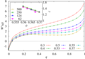
Figure 1: (Color online) Derivative of the replica potential, $\hat{W}^{\prime}(q)$ obtained as  (9) at different packing fractions. Inset: Phase diagram $(\epsilon,\phi)$ extracted from the Maxwell construction for different system sizes. The errors are computed using the jackknife method.

As was discussed before, the first order transition line is expected to extend within the liquid phase in the presence of an external field but terminates in a critical point. This point cannot be detected by the Maxwell construction so we propose a different approach. Besides, the coexistence line can be extended beyond the critical point by what is known as the Widom line Widom (1965) that is characterized by $W^{\prime\prime\prime}(q)=0$. With this idea in mind, we look for the $\epsilon$ value that makes the distribution $P_{\epsilon}(q)$ balanced. In particular, we seek the $\epsilon$ that causes the skewness to vanish. In the metastability region, the $\epsilon(\phi)$ line obtained with this method (see Fig. 3) is numerically indistinguishable from the one computed using the Maxwell construction (as we would expect in the infinite volume limit). Indeed, it finds the field at which the probability distribution function has two peaks of equal probability. Once it is understood that this line contains the second order transition point, we can try to infer its location by seeking universal behavior. At least in mean field, this point should belong to the $d=3$ Ising model universality class Franz and Parisi (1998), which means that its critical exponents are known Pelissetto and Vicari (2002), thus making easier the computation of $\phi_{\mathrm{c}}$.

We start with the static susceptibility $\chi=N[\left\langle{q^{2}}\right\rangle-\left\langle{q}\right\rangle^{2}]$. As usual in the vicinity of a second order transition, it should scale as $\chi\propto|\phi-\phi_{\mathrm{c}}|^{-\gamma}$, in this case with $\gamma=1.2372$. As can be seen in Fig.  2 (top) we find a collapse of the data at different system sizes below $\phi_{\mathrm{c}}$ using this scaling (at least for $N\geq 124$). We obtain $\phi_{\mathrm{c}}^{N}$ from an extrapolation to a second order polynomial (see Table 1 for the fitting details). These values agree with the area of $\phi$ where the kurtosis of the distribution,

$$\kappa=\frac{\left\langle{m}\right\rangle^{4}}{\left\langle{m^{2}}\right\rangle^{2}} m=q-\left\langle{q}\right\rangle,$$ with (14)

intersects for increasing $N$, as shown in Fig. 2 (bottom). Indeed, the kurtosis is related to the Binder cumulant Binder (1982), by $B=1-\kappa/3$. Like this cumulant, the kurtosis is universal at the critical point, and its value is known $\kappa=1.6043(10)$ Blote et al. (1995). Within the precision, we can say that the data are compatible with both statements.

Figure 2: (Color online) Top: static susceptibility at different $N$ scaled as $\chi^{-1/\gamma}$ with $\gamma=1.2372$. We include the extrapolations of $\phi_{\mathrm{c}}$. Bottom: kurtosis at different $N$, the dotted line indicates the universal value for the kurtosis $\kappa=1.6043(10)$ at the critical point Blote et al. (1995).

$N$	$\phi^{N}_{\mathrm{c}}$	$\chi^{2}/\mathrm{dof}$	$\phi^{N}_{\mathrm{K}}$	$\chi^{2}/\mathrm{dof}$
62	0.5766(3)(15)	2.5/6	0.626(2)	12/11
124	0.567(3)(4)	1.7/6	0.620(2)	19.5/11
250	0.5644(13)(16)	8.5/6	0.6209(12)	8.8/11
500	0.5633(6)(17)	8.5/6	0.6187(7)	5.7/11

Table 1: Extrapolations for $\phi_{\mathrm{c}}$ and $\phi_{\mathrm{K}}$ obtained from the fits of $\chi$ (displayed in Fig. 2) and $\epsilon(\phi)$ (in Fig. 3). In both cases, data at each $N$ are obtained by fitting to a second order polynomial in $\phi$. For the fit of $\phi_{\mathrm{c}}$, we have only considered the interval $\phi\in[0.52,0.55]$, while for obtaining $\phi_{\mathrm{K}}$, we used $\phi\in[0.5275,0.57]$. The two errors in the extrapolation of $\phi_{\mathrm{c}}$ correspond to the negative and positive errors.

The quantity $\epsilon(\phi)$ carries similar information as the configurational entropy and should go to zero at the Kauzmann transition (see Berthier and Coslovich (2014) for a recent similar approach). Indeed, in the quenched case, $S_{\text{c}on}\propto q\ \epsilon$ near the transition. The approach followed here has the advantage that it is ambiguity free Angelani and Foffi (2007). The extrapolation at $\phi_{K}$ should not present problems in the quenched case (at least in the mean field limit). In the present annealed case a more careful analysis should be done. We can try to infer the location of $\phi_{\mathrm{K}}^{N}$ from a second order polynomial regression (in analogy with mean field computations Franz and Parisi (1998)), searching the point where $\epsilon(\phi)=0$ (see Fig. 3 and Table 1). Of course, this approach leads to a very crude estimation for $\phi_{\mathrm{K}}$ (the simulated values of $\phi$ are still too far away to obtain a precise limit). Nevertheless, our extrapolations seem to suggest values quite smaller than the $\phi_{\mathrm{K}}=0.635(2)$ obtained in Flenner et al. (2011) using divergence of correlation times.

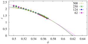
Figure 3: (Color online) Values of $\epsilon$ that guarantee a balanced distribution of $P_{\epsilon}(q)$, as function of $\phi$. We also included the fits of these curves to a second order polynomial in $\phi$. The extrapolations of $\phi_{\mathrm{K}}$ using these fits are collected in Table 1.

We have studied the equilibrium liquid-glass transition in a system of hard spheres using a tethered Monte Carlo simulation. This constrained algorithm allows us to directly compute the replica potential common in the mean field analytic computations. Using the same formalism, we are able to present clear evidences of the existence of a first order transition line in the presence of an attractive coupling between the replicas. In addition, we have investigated the critical point, showing that it belongs to the Ising model universality class as mean field calculations predicted. The emerging picture of this study is that real glass formers seem to reproduce the same schematic phase diagram as much simpler models.

We would like to thank in particular S. Franz and V. Martín-Mayor for interesting discussions. The research leading to these results has received funding from the European Research Council under the European Union’s Seventh Framework Program (FP7/2007-2013)/ERC Grant Agreement No. [247328].

References

- Ediger et al. (1996) M. D. Ediger, C. A. Angell, and S. R. Nagel, The Journal of Physical Chemistry 100, 13200 (1996).
- Leheny et al. (1996) R. L. Leheny, N. Menon, S. R. Nagel, D. L. Price, K. Suzuya, and P. Thiyagarajan, The Journal of chemical physics 105, 7783 (1996).
- Berthier and Biroli (2011) L. Berthier and G. Biroli, Rev. Mod. Phys. 83, 587 (2011).
- Adam and Gibbs (1965) G. Adam and J. H. Gibbs, The journal of chemical physics 43, 139 (1965).
- Gotze and Sjogren (1992) W. Gotze and L. Sjogren, Reports on Progress in Physics 55, 241 (1992).
- Mézard et al. (1987) M. Mézard, G. Parisi, and M. Virasoro, Spin Glass Theory and Beyond, Lecture Notes in Physics Series (Singapore: World scientific, 1987).
- Chandler and Garrahan (2010) D. Chandler and J. P. Garrahan, Annu. Rev. Phys. Chem. 61, 191 (2010).
- Kirkpatrick and Wolynes (1987) T. R. Kirkpatrick and P. G. Wolynes, Phys. Rev. B 36, 8552 (1987).
- Kirkpatrick et al. (1989) T. R. Kirkpatrick, D. Thirumalai, and P. G. Wolynes, Phys. Rev. A 40, 1045 (1989).
- Franz and Parisi (1997) S. Franz and G. Parisi, Phys. Rev. Lett. 79, 2486 (1997).
- Garrahan (2013) J. P. Garrahan, (2013), arXiv:1311.5827v1 .
- Cammarota et al. (2010) C. Cammarota, A. Cavagna, I. Giardina, G. Gradenigo, T. S. Grigera, G. Parisi, and P. Verrocchio, Phys. Rev. Lett. 105, 055703 (2010).
- Berthier (2013) L. Berthier, Phys. Rev. E 88, 022313 (2013).
- Franz and Parisi (1998) S. Franz and G. Parisi, Physica A 261, 317 (1998).
- Franz and Parisi (2013) S. Franz and G. Parisi, J. Stat. Mech. 2013, P11012 (2013).
- Biroli et al. (2013) G. Biroli, C. Cammarota, G. Tarjus, and M. Tarzia, (2013), arXiv:1309.3194 .
- Martin-Mayor (2007) V. Martin-Mayor, Phys. Rev. Lett. 98, 137207 (2007).
- Fernandez et al. (2009) L. Fernandez, V. Martin-Mayor, and D. Yllanes, Nuclear Physics B 807, 424 (2009).
- Martin-Mayor et al. (2011) V. Martin-Mayor, B. Seoane, and D. Yllanes, Journal of Statistical Physics 144, 554 (2011).
- Fernández et al. (2012) L. A. Fernández, V. Martín-Mayor, B. Seoane, and P. Verrocchio, Phys. Rev. Lett. 108, 165701 (2012).
- Torrie and Valleau (1974) G. M. Torrie and J. P. Valleau, Chemical Physics Letters 28, 578 (1974).
- Torrie and Valleau (1977) G. Torrie and J. Valleau, Journal of Computational Physics 23, 187 (1977).
- Bartels (2000) C. Bartels, Chemical Physics Letters 331, 446 (2000).
- Brambilla et al. (2009) G. Brambilla, D. El Masri, M. Pierno, L. Berthier, L. Cipelletti, G. Petekidis, and A. B. Schofield, Phys. Rev. Lett. 102, 085703 (2009).
- Mézard and Parisi (1999) M. Mézard and G. Parisi, Phys. Rev. Lett. 82, 747 (1999).
- Cardenas et al. (1999) M. Cardenas, S. Franz, and G. Parisi, The Journal of chemical physics 110, 1726 (1999).
- Widom (1965) B. Widom, The Journal of Chemical Physics 43, 3892 (1965).
- Pelissetto and Vicari (2002) A. Pelissetto and E. Vicari, Physics Reports 368, 549 (2002).
- Binder (1982) K. Binder, Phys. Rev. A 25, 1699 (1982).
- Blote et al. (1995) H. W. J. Blote, E. Luijten, and J. R. Heringa, Journal of Physics A: Mathematical and General 28, 6289 (1995).
- Berthier and Coslovich (2014) L. Berthier and D. Coslovich, (2014), arXiv:1401.5260v1 .
- Angelani and Foffi (2007) L. Angelani and G. Foffi, Journal of Physics: Condensed Matter 19, 256207 (2007).
- Flenner et al. (2011) E. Flenner, M. Zhang, and G. Szamel, Phys. Rev. E 83, 051501 (2011).
- Speedy (1993) R. J. Speedy, Molecular Physics 80, 1105 (1993).