Quantum Spin Hall Effect as $\mathbb{Z}_{2}$ Global Gauge Anomaly

Abstract

We study the relation between the quantum spin Hall effect(QSHE) and the $\mathbb{Z}_{2}$ global gauge anomaly and discover that there exists an one-to-one correspondence between them. By constructing a two dimensional non-abelian gauge theory whose non-abelian gauge field is the Berry connection induced by the Bloch wave function of the quantum spin Hall system, we prove that if the quantum spin Hall system is topologically nontrivial, the corresponding 2D gauge theory has a global gauge anomaly. We further generalize our discussion of the zero modes of the Dirac operator which play a central role in our analysis. We find that the classical ”spin” Hall effect also contains a $\mathbb{Z}_{2}$ topological invariant which is not noticed before as far as we know.

I Introduction

Topological insulator (TI) discovered by C. L. Kane and E. J. MeleKane is a new state of matter whose bulk behaves like an insulator while its edge behaves like a metal. The mechanism under-lying the phenomenon is the time-reversal symmetry. The edge, where the energy gap is closed, is robust against perturbations as long as the time-reversal symmetry is preserved. This is the reason why it is named a symmetry-protected-topological(SPT) state more precisely. Each TI system is labelled by a topological invariant, which indicates its topological properties. Transition between states with different topological invariants happens only if the energy gap closes. The reader can refer to Refs. Qi-Zhang ; Qi-Zhang2 ; Hasan-Kane and references therein for a complete review.

Now, many progress on the topological insulators have been made, among which the discovery of the $\mathbb{Z}_{2}$ topological property of the quantum spin Hall states is a landmark. This $\mathbb{Z}_{2}$ topological property differs greatly from those ordinary quantum Hall effects which are $\mathbb{Z}$ classified. It states that in the Brillouin zone, there can stably exist only one or zero Dirac-cone-like point which will be defined more precisely below. The presence of more than one such point is non-stable, implying that we can perturb the parameters so that they can be annihilated and created in pairs, until there are only one pair or none remains in the Brillouin zone. Then, the authors of QHZ proposed another formalism to describe the quantum spin Hall effects, and made a generalization to high dimensional topological insulators using a Chern-Simons field theory. The method is mainly dimensional reduction, and they acquired a seemingly different set of topological invariants. WangZ.Wang proved that in three dimensions, the two set of topological invariants are equivalent, which unified the two different approaches.

All above achievements are based on non-interacting systems, and the band structure analysis is valid. However, when interaction is taken into consideration, many of the above discussion fail. Some results have been acquired by using Green functionWang ; Wang1 ; Wang2 . But much more are still unknown. Another way to understand the interacting phenomena is to study anomalies related to topological states since anomalies are not restricted to non-interacting systems. It has long been believed that various anomalies and topological phases are in one-to-one correspondence. In Ref.Ryu , the authors made a summary of the correspondence between $\mathbb{Z}$ topological states and anomalies, but the situation for most $\mathbb{Z}_{2}$ states is unclear. This is our primary motivation in this work and we propose a relationship between the quantum spin Hall effect (QSHE) $\mathbb{Z}_{2}$ invariant and the global gauge anomaly.

The article is organized as follows. In Sec.II, we give a brief review according to Kane-Mele’s workKane-Mele on a $\mathbb{Z}_{2}$ topological invariant. In Sec.III, we summarize some main features of the global gauge anomaly which are relevant to our discussion. In Sec.IV, the relationship between the gauge anomaly and the $\mathbb{Z}_{2}$ topological invariant is established. As an application of our formalism, in Sec.V, we discuss the Morse theory associated to the Dirac operator and find a bonus, which indicates that the classical ”spin” Hall effect also have a $\mathbb{Z}_{2}$ internal topological invariant as in the quantum case predicted nearly a decade ago. Finally, we give some discussion and conclusion, and propose some further topics to be investigated in Sec.VI.

II Topological $\mathbb{Z}_{2}$ invariants of a $2+1$ dimensional quantum spin Hall system

Before studying the relation between the quantum spin hall effect and the global gauge anomaly, it is beneficial to give a brief review on both theories.

According to the work by C. L. Kane and E.J. MeleKane-Mele , we first consider a two spatial dimensional system, without interaction, with a Hamiltonian $H(k)$. The corresponding Bloch wave functions $|k,\alpha\rangle$ are given by the eigen-equation

$$H(k)|k,\alpha\rangle=E_{\alpha}|k,\alpha\rangle.$$ (1)

We require the Hamiltonian to be the time-reversal invariant: $\Theta H(k)\Theta^{\dagger}=H(-k)$, where the time-reversal operator is $\Theta=TK$ and $K$ is a complex conjugate operator. Due to such a symmetry, both $|-k,\alpha\rangle$ and $\Theta|k,\alpha\rangle$ are solutions of an eigen-equation with an eigenvalue $E_{\alpha}$. They may be related by fixing the gauge condition as $|-k,\alpha\rangle=\Theta|k,\alpha\rangle$.

In order to define topological invariants, it is convenient to introduce two concepts: an odd space and an even space. The even space is a set of points in momentum space satisfying the condition: $\Theta H(k)\Theta^{\dagger}=H(-k)=H(k)$, which means that $\Theta|k,\alpha\rangle$ and $|k,\beta\rangle$ are not perpendicular to each other, while the odd space is a set that the two vectors are mutually orthonormal. The two space can be distinguished by considering whether the matrix $\langle k,\alpha|\Theta|k,\beta\rangle$ equals to zero(an odd space) or not(an even space).

Now, we list some properties of the matrix $\langle k,\alpha|\Theta|k,\beta\rangle$:

1. It is anti-symmetric, $i.e.~{}\langle k,\alpha|\Theta|k,\beta\rangle=-\langle k,\beta|\Theta|k,\alpha\rangle$. And we can define its Pfaffian as $P(k)=Pf(\langle k,\alpha|\Theta|k,\beta\rangle)$.

2. The points in an odd space appears in pairs at $(k,-k)$.

3. Since points in an odd space are in pairs, when there are two such pairs in the Brillouin zone, it is always possible to the move them together to annihilate them.

From the above discussion, we know that the number of pairs in an odd space can only be zero or one. The two cases cannot be deformed to each other since if $k$ wants to meet $-k$, the only choice is to meet at the origin, which obviously belongs to an even space. Therefore, there is a topological obstruction between the two phases. So, it is possible to define the number of pairs in an odd space as a topological invariant which distinguishes the two cases. In order to calculate it, it is convenient to express it as a contour integral with the help of the Cauchy theorem:

$$I=\frac{1}{2\pi i}\oint_{halfBZ}d\vec{k}\cdot\nabla_{\vec{k}}\log(P(k)+i\delta)~{}(mod\ 2).$$ (2)

Integrating over half of the Brillouin zone means that we only have to count points instead of pairs with $\delta$ being a small parameter making the integral convergence.

In the above discussion, we only require the Hamiltonian to be time-reversal symmetric, and do not impose any other restrictions, such as a rotational symmetry or the specific form of the Hamiltonian. So the $\mathbb{Z}_{2}$ topological properties are quite universal.

III A brief review of the global gauge anomaly

The global gauge anomaly, especially an $SU(2)$ gauge anomaly, was originally discovered by E. WittenWitten by considering a chiral Weyl fermion minimally coupled to an $SU(2)$ gauge field. The action of the model is

$$S=\int d^{4}x\left[\bar{\psi}i\not{D}\psi-\frac{1}{2g^{2}}\textrm{tr}F_{\mu\nu}F^{\mu\nu}\right]$$ (3)

where $\psi(x)$ is a Weyl fermion, $A_{\mu}$ is an $SU(2)$ gauge field, $D_{\mu}=\partial_{\mu}+igA_{\mu}$ is a covariant derivative and $F_{\mu\nu}=\partial_{\mu}A_{\nu}-\partial_{\nu}A_{\mu}-ig[A_{\mu},A_{\nu}]$ is the field strength. In order to quantize the theory, we consider the partition function:

$$Z = \int d\psi d\bar{\psi}\int dA_{\mu}$$ (4)

$$\times\exp\left\{-\int d^{4}x\left[\bar{\psi}i\not{D}\psi-\frac{1}{2g^{2}}trF_{\mu\nu}F^{\mu\nu}\right]\right\}.$$

Integrating over the fermion degree of freedom, we may get an effective low energy action only in terms of the gauge fields. To do the integration, we consider the case for a Dirac fermion coupled to an $SU(2)$ gauge field. For this case, the integration is well known to be $\det(i\not{D})$. Since the number of Weyl spinors is half of the number of Dirac spinors, thus, the integration is $\pm(\det(i\not{D}))^{\frac{1}{2}}$. Notice that the sign at the front cannot be fixed globally. In order to settle this ambiguity, one needs to choose a specific configuration, say, the vacuum $A^{0}_{\mu}$, to be positive and other configurations related to this via a gauge transformation $A_{\mu}=U^{-1}A^{0}_{\mu}U-iU^{-1}\partial_{\mu}U$, where $U\in SU(2)$.

In four dimensions, more generally for any even dimension, aside from all the Gamma matrices, there is an additional one $\Gamma_{5}$ which is proportional to the product of all Gamma matrices and anti-commute with all others. Thus, when $\psi$ is an eigenstate with energy $E$, $\Gamma_{5}\psi$ is also an eigenstate with the opposite energy $-E$. Therefore, the energy spectrum is symmetric with respect to the origin. Considering that $\det(i\not{D})$ is just the product of all eigenvalues, $\pm(\det(i\not{D}))^{\frac{1}{2}}$ is determined by a product of half of the spectrum, picking one value from each pair. In order to let the sign in the front to be definitive, one needs to exclude all the zero eigenvalues from the definition of the determinant.

From the above discussion, one can find that there exists some $U$ such that $(\det i\not{D}[A])^{\frac{1}{2}}=-(\det i\not{D}[A^{U}])^{\frac{1}{2}}$ and others $(\det i\not{D}[A])^{\frac{1}{2}}=(\det i\not{D}[A^{U}])^{\frac{1}{2}}$, which is known as a global gauge anomaly. More detailed discussions show that the measures of $U$ in both cases turn out to be the same. The consequence of such a gauge anomaly can lead to the above partition mathematically ill-defined. But we do not spare our efforts on it. As Witten pointed out, the mathematical origin of a global gauge anomaly lies in the fact that

$$\pi_{4}(SU(2))=\mathbb{Z}_{2},$$ (5)

where the subindex $4$ is the dimension of space-time. Equation (5) shows the appearance of an anomaly is determined by the topological property of the gauge group. Indeed, when we deform the transformation matrix a little, we can prove that the resulting gauge field belongs to the same class as the original one. The result also tells us that the global gauge anomaly can occur in other even dimensions since Clifford algebra can have symmetric energy spectrum only in even dimensions and its square root can have a definitive meaningNakahara .

In the next section, we will in fact use a more general case

$$\pi_{2}(G)=\mathbb{Z}_{2}$$ (6)

where the subindex $2$ is the dimension of momentum space and $G$ is the symmetry group of a QSHE Hamiltonian. It is worth to note that Eq.(6) is true and can be proven almost the same as for the four dimensional case.

IV $\mathbb{Z}_{2}$ topological invariant in a QSHE from a global gauge anomaly

The similarities of the topological property between the QSH and the gauge anomaly makes us to ask whether there exists a relation between them and what it is. Indeed, by studying, we find that the system described by a two dimensional Lagrangian which carries the topological information of the QSH system exhibits a global gauge anomaly. In the following, we show how they are obtained.

Firstly, we display some correspondence between a QSHE and a global gauge anomaly:

• Field contents: Bloch wavefunction $|k,\alpha\rangle$ or Pfaffian$(\langle k,\alpha|\Theta|k,\beta\rangle)$ $\longleftrightarrow$ Nonabelian gauge field $A_{\mu}$.

• Base Manifold: 2D momentum space $\longleftrightarrow$ Even dimensional D space-time.

• Symmetry: Time Reversal Symmetry $\longleftrightarrow$ Chiral-Antichrial Symmetry.

• Topological origin: $\pi_{2}(G)=\mathbb{Z}_{2}$, where $H\in G$ $\longleftrightarrow$ $\pi_{D}(G)=\mathbb{Z}_{2}$, where $A_{\mu}\in G$.

Although there appears to be some difference, the similar topological origin indicates both are determined by the homotopic group of some group which the field content belongs to. This motivates us to find a connection between them. In order to connect the non-abelian gauge field with the Bloch wavefunction, the most natural way is to define the Berry connection/gauge field as follows:

$$A_{\mu}^{\alpha\beta}(k)=-i\langle k,\alpha|\partial_{\mu}|k,\beta\rangle.$$ (7)

Notice that it is indeed a gauge field because when the Hamiltonian takes an unitary transformation as $H(k)\rightarrow UH(k)U^{-1}$, the Bloch wavefunction is transformed by $|k,\alpha\rangle\rightarrow U_{\alpha\beta}|k,\beta\rangle$ and the Berry connection is transformed by $A_{\mu}^{\alpha\beta}(k)\rightarrow(U^{*}A_{\mu}U^{*\dagger}-iU^{*}\partial_{\mu}U^{*\dagger})^{\alpha\beta}$, which indicates that $A_{\mu}$ transforms similarily as a gauge field. From the above argument, we may find that the representation of the Hamiltonian and that of the Berry connection belong to the same group. Therefore, the topological origin of both theories exactly matches — both of them are determined by the symmetry group which the non-abelian gauge field belongs to.

Although the origin is the same, it is still worth to study whether there is a one-to-one correspondence between a topological trivialness/nontrivialness and a gauge anomaly appearance/vanishness. So further investigations are needed.

As we know, for any antisymmetric matrix, $[Pf(X)]^{2}=\det(X)$, so $Pf(X)=\pm[\det(X)]^{\frac{1}{2}}$, where the sign $\pm$ is indefinitive. In order to understand the role which the Berry connection is playing in the $\mathbb{Z}_{2}$ topological invariant, we substitute it into Eq.(2), the invariant can be given as

$$I = \frac{1}{4\pi i}\oint_{halfBZ}d\vec{k}\cdot\nabla_{\vec{k}}\log(\det(\langle k,\alpha|\Theta|k,\beta\rangle))(mod\ 2)$$

$$= \frac{1}{4\pi i}\oint_{halfBZ}d\vec{k}tr([^{*}\langle k,\beta|T^{\dagger}\partial_{\vec{k}}|k,\alpha\rangle]^{*}+\langle k,\alpha|\partial_{\vec{k}}T|k,\beta\rangle^{*})[\frac{1}{\langle k,\alpha|T|k,\beta\rangle^{*}}](mod\ 2).$$

Here the indefinitive sign disappears due to the $\nabla$ operator. The first term in the bracket can be rewritten as

$$[^{*}\langle k,\beta|T^{\dagger}\partial_{\vec{k}}|k,\alpha\rangle]^{*}=iS^{\beta\gamma}(k)[\vec{A}^{\gamma\alpha}(k)]^{*},$$ (9)

where we define $S^{\alpha\beta}=\langle k,\alpha|\Theta|k,\beta\rangle$.

As for the second term, some special care is needed. From the second section, we have chosen the gauge fixing condition as $|-k,\alpha\rangle=T|k,\alpha\rangle^{*}$ and to expand it in terms of gauge field, we need to use this identity. One should pay attention to the fact that the identity can only be defined locally on the base manifold, otherwise, as one can check without much effort, the contributions of the first term and the second term just cancel with each other, indicating that the QSHE system is always topological trivial. We have to remark that the argument in the second section does not solve this problem since the equation only applies to the proof of the orthonormal condition, which is a purely local argument. But in this case, we have to integrate over the Brillouin zone and thus a global effect emerges. The simplest solution to tackle the problem is to divide the Brillouin zone into two parts, namely $A$ and $B$. In part $A$, the above condition is valid, while in part $B$, the Bloch wave function is related to that of $A$ via a transformation matrix $t$: $|k,\alpha\rangle_{A}=t^{\alpha\beta}|k,\beta\rangle_{B}$. When $k$ is in part $A$, the second term can be given as

$${}_{A}\langle k,\alpha|\partial_{\vec{k}}T|k,\beta\rangle^{*}_{A}=-iS^{\alpha\gamma}_{A}(k)\vec{A}^{\gamma\beta}_{A}(-k).$$ (10)

When $k$ is in part B, the second term can be expressed as

$${}_{B}\langle k,\alpha|\partial_{\vec{k}}T|k,\beta\rangle^{*}_{B} = t^{*\delta\gamma}S_{B}^{\alpha\gamma}(\partial_{\vec{k}}t^{\delta\beta})-t^{\delta\beta}\partial_{\vec{k}}t^{*\delta\gamma}S_{B}^{\alpha\gamma}$$ (11)

$$-it^{\delta\beta}t^{*\delta\gamma}S_{B}^{\alpha\eta}\vec{A}_{B}^{*\eta\gamma}(k).$$

Substituting all Eqs.(9)-(11) into Eq.(LABEL:4.2_II), we obtain the topological invariant as follow

$$I = \frac{1}{2\pi i}\oint_{\partial B}d\vec{k}\textrm{tr}(t^{*\delta\gamma}\partial_{\vec{k}}t^{\delta\beta})(mod\ 2)$$ (12)

$$= \frac{1}{2\pi i}\oint_{\partial B}d\vec{k}\textrm{tr}(t^{\dagger}\partial_{\vec{k}}t)(mod\ 2).$$

Here, its physical meaning is obvious: when momentum $k$ travels around the part $B$ once, $t$ gains an additional phase angle, which is integer times $2\pi i$. Notice that $B$ in this case may not be simply connected, but it will not affect our analysis because we can add different branches of integral provided that we carefully keep the same orientation among them. The topological invariant just counts this integer. Moreover, when we set $A_{\mu}^{0}$ to be a trivial Berry connection, and let $t$ be the gauge transformation, we get a new Berry gauge field. The invariant can be expressed in terms of the new gauge field via

$$I=\frac{1}{2\pi}\oint_{BZ}\textrm{tr}[A](mod\ 2).$$ (13)

We have to remark here that this result was previously obtained by L. Fu and C. KaneFu-Kane from a more complicated method. Here we acquire it by a simple and direct calculation. With the help of this simplified invariant, we can state an important property which directly leads to the equivalence between the two theories topologically.

If the two Hamiltonians $H_{1}(k)$ and $H_{2}(k)$ describe QSHE systems, they determine two Berry connections $A_{1}(k)$ and $A_{2}(k)$, as well as two transformation matrices $t_{1}$ and $t_{2}$. They correspond to two topological invariants

$$I_{1}=\frac{1}{2\pi i}\oint_{\partial B}d\vec{k}\textrm{tr}(t^{\dagger}_{1}\partial_{\vec{k}}t_{1})(mod\ 2)=0$$

$$I_{2}=\frac{1}{2\pi i}\oint_{\partial B}d\vec{k}\textrm{tr}(t^{\dagger}_{2}\partial_{\vec{k}}t_{2})(mod\ 2)=1.$$ (14)

We define a new Berry connection connecting the above two adiabatically as $A_{s\mu}=(1-s)A_{1\mu}+sA_{2\mu}$ and $s\in[0,1]$. All the above are based on the information provided by the QSHE. Now, we define a two dimensional theory whose Lagrangian is

$$\mathcal{L}=\bar{\psi}i\not{D}\psi-\frac{1}{2e^{2}}\textrm{tr}F_{\mu\nu}F^{\mu\nu},$$ (15)

$F_{\mu\nu}$ is the strength field induced by the Berry gauge field and $\psi$ is a Weyl spinor. The Dirac equation, defined on the momentum space, can be written as

$$i\not{D}[A_{s}]\psi_{s}=\lambda_{s}\psi_{s}.$$ (16)

As the $s$ runs adiabatically from $0$ to $1$, we can follow the tracks of the eigenvalue $\lambda$. In the following, we prove that if there exist odd number of eigen-spectral lines flowing across zero, they lead to the fact that

$$(\det i\not{D}^{\prime}[A_{1}])^{\frac{1}{2}}=-(\det i\not{D}^{\prime}[A_{2}])^{\frac{1}{2}},$$ (17)

where the prime on Dirac operators means they are induced by the Dirac fermions, not the Weyl fermions. Therefore, there is a global gauge anomaly in the system defined by Lagrangian (15).

Here, we need to make a few remarks that the Dirac equation (16) and the Lagrangian (15) stated above are slightly different from normal ones, which are defined on the momentum space.

Since the topological invariant is $\mathbb{Z}_{2}$ valued, any even number can be adiabatically deformed to zero; similarly, any odd number to one. Thus we may remove the $(mod\ 2)$ operator and just set the integrals to be one and zero. What is more, since $H_{1}(k)$ is topological trivial, we may set the corresponding Berry connection and the transformation matrix identically as zero. Therefore, we may set the gauge transformation relating $A_{1}$ and $A_{2}$ as $t\equiv t_{2}$, $i.e.$ $A_{2\mu}=t^{*}A_{1\mu}t^{*\dagger}-it^{*}\partial_{\mu}t^{*\dagger}$. For the two dimensional case, according to the Atiyah-Singer index theoremFriedan ; Vafa

$$\nu_{+}-\nu_{-}=\frac{1}{2\pi}\int_{BZ}\textrm{tr}F=\frac{1}{2\pi}\oint_{BZ}\textrm{tr}A,$$ (18)

we can obtain

$$\nu^{s}_{+}-\nu^{s}_{-} = \frac{s}{2\pi}\oint_{\partial BZ}d\vec{k}\textrm{tr}(t^{\dagger}\partial_{\vec{k}}t)$$ (19)

$$= \frac{s}{\pi}\oint_{\partial B}d\vec{k}\textrm{tr}(t^{\dagger}\partial_{\vec{k}}t)$$

$$= 2sI_{2}=2s,$$

where in the second line, we switch the integration domain only in part $B$. On the left hand side, $\nu_{+}$ counts the number of zero modes of the dimensional kernel of the left hand Dirac operator $iP_{+}\not{D}$ where $P_{+}=\frac{1}{2}(1+\gamma^{2+1})$Nakahara . Similar definition works for $\nu_{-}$. Here, we will use a more convenient and straight forward way to compute the index with the help of Fig.1.

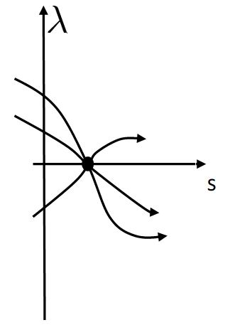
Figure 1: Zero modes of Dirac operator at $s$. This zero point consists of three spectral flows: two from the above and one from below, i.e. $\nu_{+}=2$ and $\nu_{-}=1$

$\nu_{+}$ represents the number of flows from up to down and $\nu_{-}$ from down to up. Therefore, the left hand side must be an integer. As for the right hand side, $s\in[0,1]$, it means that $s$ can only be $0$ or $\frac{1}{2}$ or $1$. When $I_{2}=-1$, $s$ reverse its sign. We claim that $s=\frac{1}{2}$ is the only solution in the present case because $s=0$ or $s=1$ implies that there are zero modes in the original spectrum, inconsistent with our assumption. Therefore, when $s$ goes from $0$ to $1$, the only possible point for zero mode is at $s=\frac{1}{2}$.

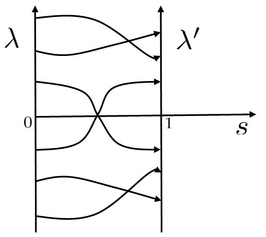
Figure 2: A typical flowing spectrum. The horizontal axis represents parameter varying from zero to one. The vertical axis represents eigenvalues. Eigenvalues run as the parameter $s$ vary.

Fig.2 is a typical flowing spectrum of that Dirac operator. The spectrum is symmetric with respect to the zero value, as previously stated. As $s$ varies from 0 to 1, the eigenvalues rearrange to form a new spectrum. Although the overall distribution seems unchanged, the relative position may vary. In order to acquire the spectrum of an operator induced by a Weyl fermion, we can choose one eigenvalue from each pair. Fig.3 are a pair of Dirac and Weyl spectrum.

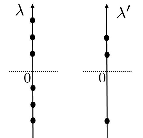
Figure 3: An example of Dirac and Weyl spectrum. The left is Dirac and the right is Weyl.

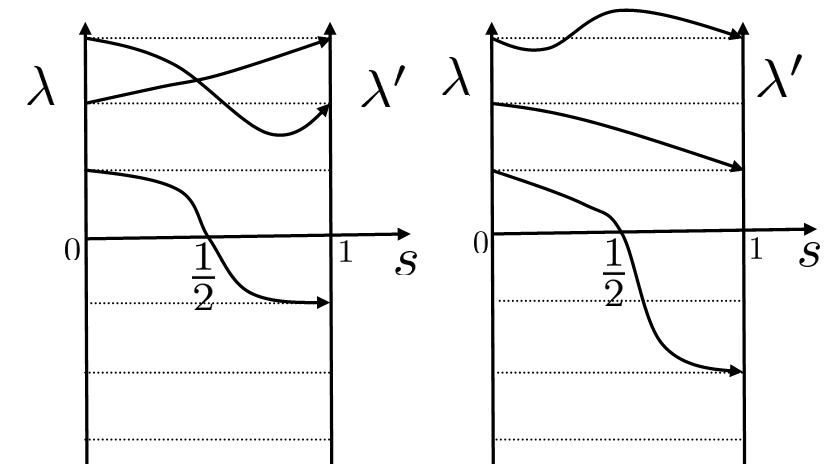
Figure 4: When there is only one eigenvalue running across the horizontal axis, the product of all the eigenvalues reverse sign. Here we only list two possibilities.

Now, we search for all the solutions satisfying $\nu_{+}-\nu_{-}=1$ and prove that all these solutions are with a global gauge anomaly.

First, when there is one spectral line running across horizontal axis, as shown in Fig.4. In order to guarantee the spectrum to be Weyl, the only possibilities are those which satisfies that the product of all the eigenvalues being the same absolute value of the original ones. Moreover, since there is only one eigenvalue which reverses its sign, though its absolute value may change as in Fig.2, the product is exactly the minus of the Original one, which is equivalent to the identity

$$(\det i\not{D}^{\prime}[A_{1}])^{\frac{1}{2}}=-(\det i\not{D}^{\prime}[A_{2}])^{\frac{1}{2}}.$$ (20)

So, for this case, we prove that there is a global gauge anomaly.

Second, when there are two eigenvalues flowing across the horizontal axis, the two can both go from up to down, which means $\nu_{+}-\nu_{-}=2$, or in the opposite direction, i.e. $\nu_{+}-\nu_{-}=-2$. Another possibility is that one from up to down and the other from down to up, i.e. $\nu_{+}-\nu_{-}=0$. All the above three cases do not match the condition $\nu_{+}-\nu_{-}=1$.

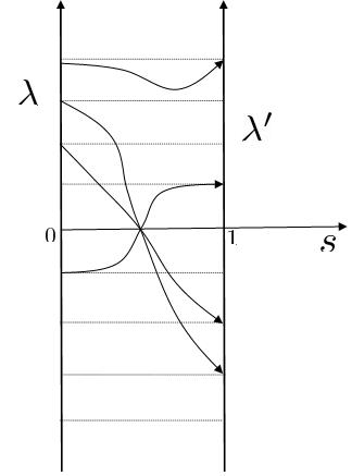
Figure 5: When there are only three eigenvalues running across the horizontal axis. Here only draw one particular diagram. There are two lines goes from up to down and one from down to up, which preserves $\nu_{+}-\nu_{-}=1$. Effectively, there are only one eigenvalue reverse the sign, and all others mutually rearranged.

Then, when there are three eigenvalues flowing across the horizontal axis, as shown in Fig.5, similar analysis as in the first case can tell there is a global gauge anomaly.

Finally, for any odd number of lines crossing the horizontal axis, it is not difficult to draw the conclusion that for all the solutions satisfying $\nu_{+}-\nu_{-}=1$, there is a global gauge anomaly. For any even number of lines crossing the horizontal axis, there does not exist a solution satisfying $\nu_{+}-\nu_{-}=1$. It ends the prove of our equivalence property.

Up to now, we can conclude that the non-trivial topological quantum spin Hall effect corresponds to the global gauge anomaly whose gauge field is induced by the Berry connection of the former. Here, a comment on global gauge anomaly may be helpful. In a paperAlwis , the author suggested that an $SU(2)$ global gauge anomaly can be seen as an $U(1)$ anomaly by observing that the special $U(1)$ element $e^{i\pi}$ is also the center of an $SU(2)$ transformation. So an $SU(2)$ global gauge anomaly can also be viewed as a more familiar $U(1)$ anomaly as in the case of a $3D$ topological insulator. However, here, the gauge group we are discussing is more complicated than an $SU(2)$. But the existence of the above correspondence may help us understanding our formulation by studying the $3D$ case.

V Morse theory and the classical spin Hall effect

In this section, we discuss the Witten-deformed Dirac indexWitten2 and find that $\mathbb{Z}_{2}$ index for quantum theory is the same as that for the classical theory, and therefore we conjecture that the classical ”spin” Hall effect also contains the $\mathbb{Z}_{2}$ topological property, which have not been discussed as far as we know.

In the above, we have shown a crucial formula,

$$\nu_{+}-\nu_{-}=\frac{1}{2\pi}\oint_{BZ}\textrm{tr}A,$$ (21)

which is a specific example of Atiyah-Singer index theorem. In fact, the left and right hand side of the equation are two different limits of a same quantityFriedan , $i.e.$

$$\textrm{ind}(\not{D}[A])=\textrm{tr}\gamma_{5}e^{-\beta\not{D}^{\dagger}\not{D}}=\left\{\begin{array}[]{ll}\nu_{+}-\nu_{-},&\hbox{$\beta\rightarrow\infty$;}\\ \\ \frac{1}{2\pi}\oint_{BZ}\textrm{tr}A,&\hbox{$\beta\rightarrow 0$.}\end{array}\right.$$ (25)

The index for Dirac operator reminds us the similar supersymmetric case

$$\textrm{Tr}(-1)^{F}e^{-\beta Q^{\dagger}Q}$$ (26)

where $Q$ is the supersymmetry operator. These two index can be related by the following map:

$$(-1)^{F} \rightarrow \gamma_{5},$$ (27)

$$\not{D} \rightarrow Q,$$ (28)

$$H=\not{D}^{\dagger}\not{D} \rightarrow H=Q^{\dagger}Q.$$ (29)

E. Witten, in his seminal paper, derived the Morse inequality with the help of supersymmetric quantum mechanics of the later case. Here we apply his idea to the discussion of the Dirac index. By parallel analysis, we can also derive the Morse inequality.

For convenience, we set the representation of the Dirac matrix satisfying $\gamma_{5}=\textrm{diag}(I,-I)$. The Dirac operator can be expressed as the form

$$\not{D}=\left(\begin{array}[]{cc}0&\not{D}_{-}\\ \not{D}_{+}&0\\ \end{array}\right),$$ (32)

where $\not{D}_{-}^{\dagger}=-\not{D}_{+}$, and $\not{D}_{\pm}=D_{i}\Gamma^{i}_{\pm}$. In the previous analysis, we focus on the Dirac equation

$$i\not{D}_{+}\psi_{+}=\lambda\psi_{+}.$$ (33)

And other part is similar, $i.e.$

$$i\not{D}_{-}\psi_{-}=-\lambda\psi_{-}.$$ (34)

To counting the number of Dirac zero modes which is of interest in the previous section, one only needs to count the chiral part or anti-chiral part. Here, we will mainly focus on the ground state of the Hamiltonian

$$H =\textrm{tr}\not{D}^{\dagger}\not{D}$$ (35)

$$=-(\not{D}_{-}\not{D}_{+}+\not{D}_{+}\not{D}_{-})$$

$$=-2D^{i}D_{i}.$$

We can show that the number of ground state of the Hamiltonian equals to the number of the zero modes of the Dirac equation. If a zero mode of a Dirac equation $\not{D}_{+}\psi=0$ with $\not{D}_{-}\psi=0$ is simultaneously true, it is obvious that $\psi$ is also the ground state of the Hamiltonian $H$. Conversely, if $H\psi=0$, by integrating by parts, we can obtain

$$\int\psi^{*}H\psi=-2\int\psi^{*}D_{i}D^{i}\psi=2\int|D_{i}\psi|^{2}=0,$$ (36)

which immediately leads to $D_{i}\psi=0$. Thus, $\psi$ is also the zero mode of Dirac operator. Therefore, it is proven that we may consider the ground states or the vacuum of the Hamiltonian instead of counting the number of the Dirac zero modes. We should point out here that this equivalence is only valid in the two dimensional case.

According to Witten’s idea, we can deform the Dirac operator slightly as the following

$$\not{D}_{+}\rightarrow\not{D}_{+}^{t}=e^{-ht}\not{D}_{+}e^{ht},$$ (37)

$$\not{D}_{-}\rightarrow\not{D}_{-}^{t}=e^{ht}\not{D}_{-}e^{-ht}.$$ (38)

Of course, deformations in this way neither introduce extra zero ground states nor eliminate any. We may express the deformed Dirac operator by introducing two more physical raising and lowering operators

$$\not{D}_{+}^{t}=\not{D}_{+}+tD_{i+}ha^{i},$$ (39)

$$\not{D}_{-}^{t}=\not{D}_{-}+tD_{i-}ha^{i*}.$$ (40)

Here we may regard $a^{i}$ and $a^{j*}$ as rising and lowering one chirality of the following operator respectively. Substituting above into the Hamiltonian $H$, one can rewrite the Hamiltonian as the following form

$$H=-\not{D}_{-}\not{D}_{+}-\not{D}_{+}\not{D}_{-}+t^{2}(iD_{i}h)^{2}+tiD_{i}h\ iD_{j}h[a^{i},a^{j*}],$$ (41)

where we let $i$ be explicit because the $iD$ is Hermitian and the product with its conjugate is positive definited. One can immediately see from the equation that the Hamiltonian is composed of three parts, the kinetic term, the oscillator potential term, and the quantum correction. The first two terms are purely classical contributions. In order to extract out the classical parts, it is natural to consider large $t$ limit under which case the quantum correction, proportional to $t$, is suppressed down by the quadratic of $t$. Under this limit, we may expand the eigenvalue $\lambda$ of the total Hamiltonian by the order of $1/t$ as

$$\lambda(t)=t\left[A+\frac{B}{t}+\frac{C}{t^{2}}+\cdots\right].$$ (42)

The $t$ in the front of Eq.(42) is analogous to the solution of the free oscillator which has the form of $\omega(n+1/2)$ where $\omega$ in this situation is $t$. $A$ represents the classical contribution and other terms are the quantum effects.

For the ground state of the Hamiltonian, corresponding to $\lambda(t)=0$, it implies that $A$, the energy eigenvalue, corresponding the classical system, reaches its vacuum. However, the reverse case is not necessarily true. Namely, for $A=0$, one cannot obtain that the total quantum eigenvalue is zero. With this consideration, one can write down an inequality

$$\#\{\lambda_{p}=0\}\leq\#\{A_{p}=0\},$$ (43)

where $p$ means the chirality of the particle and the inequality is valid for any $p$. It means that the number of quantum vacuum is always less than that of the classical vacuum. Actually, as Witten claimed, the number of vacuums on both sides can be interpreted as the Betti-number and the Morse-index, respectively. The argument will not be discussed here. The above inequality can be rewritten as

$$B_{p}\leq M_{p},$$ (44)

which is the weak form of the Morse inequality.

There is one more fact that the Morse inequality has a strong form, saying

$$\sum_{p}M_{p}t^{p}-\sum_{p}B_{p}t^{p}=(t+1)\sum_{p}Q_{p}t^{p},$$ (45)

where $Q_{p}$’s are non-negative integers. Since, in the previous section, we only count the total number of zero modes of the Dirac operator, we should sum over all possible chirality. This motivates us to set $t=1$. For $t=1$, the equality (45) becomes

$$\sum_{p}M_{p}-\sum_{p}B_{p}=2\sum_{p}Q_{p},$$ (46)

which gives us a great surprise. Since $B_{p}$, which is the number of quantum vacuum, is stable only up to $\mathbb{Z}_{2}$, and the right hand side of Eq.(46) is always an even integer, so the number of classical vacuum is stable up to $\mathbb{Z}_{2}$ also. Paraphrasing it into the condensed matter physics language, the classical ”spin” Hall effect also contains the $\mathbb{Z}_{2}$ topological invariant which characterizes its topological nature. It is worth to note that in classical theory, there is no concepts like spin, so we put a quotation mark on the spin. It is still difficult to construct this classical system for the time being. The method we try to use is to construct some kind of index which counts the number of states satisfying $\langle k,\alpha|\Theta|k,\beta\rangle=0$. Then, usually such index can be written as some path integral. Then classical version of this is to use the saddle point approximation. Then we can investigate such quantity to see whether this is a $\mathbb{Z}_{2}$ quantity. However, we are still not clear about how to construct the index. We are trying to solve this and find other more accessible ways at the same time. Moreover, this phenomenon is not covered in the existing literatures, and more concrete analysis in terms of the topological properties of the classical systems indicated by the above is expected to be further investigated.

VI Discussion and Conclusion

In this article, we prove that the topological nontrivial quantum spin Hall effect is equivalent to the $\mathbb{Z}_{2}$ global gauge anomaly of the system described by the Lagrangian (15). The Lagrangian is somewhat similar to that describing massless QCD, which also contains a pair of fermions and non-abelian gauge fields. But the difference is that the former is defined on the momentum space, and the fermions is a Weyl. Moreover, the non-abelian gauge group, in order to generate a $\mathbb{Z}_{2}$ non-trivial topology, cannot be chosen arbitrarily. In fact, the symmetry group is determined by the CPT symmetry of the Hamiltonian. Similar to the fact that there exist fractional charge in QCD, the fractional excitations in the QSHE also appearLan , which needs further investigation.

As we mentioned before, the appearance of a global gauge anomaly can occur in any even dimension, therefore, we expect that we may find similar correspondence between a $4+1$ dimensional topological insulator and a $4d$ non-abelian gauge theory(Euclidean QCD). Moreover, from the approach of Ref.QHZ , we find the $2+1$ dimensional topological invariant, which is obtained by a dimensional reduction, is

$$P_{3}(\theta)=\frac{1}{2\pi}\oint d\phi\Omega_{\phi},$$ (47)

where $\Omega_{\phi}$ is defined in Eq.(112) in Ref.QHZ . It is of the same form as (13). Therefore, we can conclude that our formalism can also be applied to a Chern-Simons field theory approach. However, we should mark that the $3+1$ dimensional case, which is not included in our formalism, is related to the $U(1)$ chiral anomaly. Other $\mathbb{Z}$ SPT cases were already found to be corresponding to various anomalies. The relationship between an anomaly and most of other $\mathbb{Z}_{2}$ topological SPT states is still not clear yet. We hope that our article can provide some inspiration toward the understanding of these issues.

Lastly, through some analysis of the spectrum of the deformed Hamiltonian (41), we find that the classical ”spin” Hall effect also has a $\mathbb{Z}_{2}$ topological classification, which is not discovered before as far as we know. By further investigation of a classical system, we may find more interesting topological nature which may enable us a better understanding of the topology of strong correlated systems.

References

- (1) C.L.Kane, E.J.Mele, Phys. Rev. Lett. 95, 225801 (2005).
- (2) X.L.Qi, S.C.Zhang, Physics Today, 63 33 (2010).
- (3) X.L.Qi, S.C.Zhang, Rev. Mod. Phys. 83 1057 (2011).
- (4) M.Z.Hasan, C.L.Kane, Rev. Mod. Phys. 82 3045 (2010).
- (5) X.L.Qi, T.Hughes, S.C.Zhang, Phys. Rev. B 78 195424 (2008).
- (6) Z.Wang, X.L.Qi, S.C.Zhang, New J. Phys. 12 065007 (2010).
- (7) Z.Wang, X.L.Qi, S.C.Zhang, Phys. Rev. Lett. 105 256803 (2010).
- (8) Z.Wang, X.L.Qi, S.C.Zhang, Phys. Rev. B 85 165126 (2012).
- (9) Z.Wang, S.C.Zhang Phys. Rev. X 2 031008 (2012).
- (10) Shinsei Ryu, Joel E. Moore, Andreas W. W. Ludwig, Phys. Rev. B 85 045104 (2012).
- (11) C.L.Kane, E.J.Mele, Phys. Rev. Lett. 95, 146820 (2005).
- (12) E.Witten, Phys. Lett. B 117, 324 (1982).
- (13) M. Nakahara. Geometry, Topology, and Physics. A. Hilger (1990).
- (14) L. Fu, C.L.Kane, Phys. Rev. B 74 195312 (2006).
- (15) D.Friedan, P. Windey, Nucl. Phys. B 235 395 (1984).
- (16) C.Vafa, E.Witten Commun. Math. Phys. 95 257 (1984).
- (17) S. P. de Alwis, Phys. Rev. D 32 2873 (1985).
- (18) E.Witten, J. Differential Geometry 17 661 (1982).
- (19) Y.P. Lan, and S.L.Wan, J. of Phys. C 24, 165503 (2012)