Coxeter Transformations, the McKay correspondence, and the Slodowy correspondence

Rafael Stekolshchik

BIRS, 08w5060 Workshop
“Spectral Methods in Representation Theory of Algebras and Applications to the Study of Rings of Singularities”
 
September 8, 2008

In [Ebl02], Ebeling established a connection between certain Poincaré series, the Coxeter transformation C, and the corresponding affine Coxeter transformation ${\bf C}_{a}$ (in the context of the McKay correspondence). We consider the generalized Poincaré series $[\widetilde{P}_{G}(t)]_{0}$ for the case of multiply-laced diagrams (in the context of the McKay-Slodowy correspondence) and extend the Ebeling theorem for this case:

$$[\widetilde{P}_{G}(t)]_{0}=\frac{\mathcal{X}(t^{2})}{\tilde{\mathcal{X}}(t^{2})},$$

where $\mathcal{X}$ is the characteristic polynomial of the Coxeter transformation and $\tilde{\mathcal{X}}$ is the characteristic polynomial of the corresponding affine Coxeter transformation.

We obtain that Poincaré series coincide for pairs of diagrams obtained by folding:

$$\frac{\mathcal{X}(\Gamma)}{\mathcal{X}(\tilde{\Gamma})}=\frac{\mathcal{X}(\Gamma^{f})}{\mathcal{X}(\tilde{\Gamma}^{f})},$$

where $\Gamma$ is any ($A$, $D$, $E$ type) Dynkin diagram, $\tilde{\Gamma}$ is the extended Dynkin diagram, and the diagrams $\Gamma^{f}$ and $\tilde{\Gamma}^{f}$ are obtained by folding from $\Gamma$ and $\tilde{\Gamma}$, respectively.

1. The Coxeter transformation
(A bit of history)

Given a root system $\varDelta$, a Coxeter transformation (or Coxeter element) $C$ is defined as the product of all the reflections in the simple roots. (We are speaking here only about diagrams which are trees). Notations:

$h$ is the order of the Coxeter transformation (Coxeter number),

$|\varDelta|$ is the number of roots in the root system $\varDelta$,

$l$ is the number of eigenvalues of the Coxeter transformation, i.e., the number of vertices in the Dynkin diagram.

We have:

$$hl=|\varDelta|,$$

(Coxeter, [Cox51]; Kostant [Kos59]). Let $m_{i}$ be the exponents of the eigenvalues of $C$, (all the eigenvalues in the case considered here are of the form $e^{2\pi im_{j}/h}$), $|W|$ be the order of the Weyl group $W$.

Then

$$|W|=(m_{1}+1)(m_{2}+1)...(m_{l}+1),$$

(Coxeter, [Cox34] ; proved by Chevalley [Ch55] and other authors). Let $\varDelta_{+}\subset\varDelta$ be the subset of simple positive roots $\alpha_{i}\in\varDelta_{+}$,

$\beta=n_{1}\alpha_{1}+\dots+n_{l}\alpha_{l}$ be the highest root in the root system $\varDelta$. Then

$$h=n_{1}+n_{2}+...+n_{l}+1.$$

(Coxeter [Cox49]; Steinberg [Stb59]).

2. The Coxeter transformation
(bicolored partition)

A partition $S=S_{1}\coprod S_{2}$ of the vertices of the graph $\varGamma$ is said to be bicolored if all edges of $\varGamma$ lead from $S_{1}$ to $S_{2}$. (A bicolored partition exists for trees). The diagram $\varGamma$ admitting a bicolored partition is said to be bipartite.

An orientation $\varLambda$ is said to be bicolored, if there is the corresponding sink-admissible sequence.

$$\{v_{1},v_{2},~{}...,~{}v_{m},v_{m+1},v_{m+2},~{}...~{}v_{m+k}\}$$

of vertices in this orientation $\varLambda$, such that the subsequences

$$\begin{split}S_{1}=&\{v_{1},v_{2},~{}...,~{}v_{m}\},\\ S_{2}=&\{v_{m+1},v_{m+2},~{}...,~{}v_{m+k}\}\end{split}$$

form a bicolored partition, i.e., all arrows go from $S_{1}$ to $S_{2}$. The product $w_{i}\in W(S_{i})$ of all generators of $W(S_{i})$ is an involution for $i=1,2$, i.e.,

$$w_{1}^{2}=1,\qquad w_{2}^{2}=1,\qquad C=w_{1}w_{2}.$$ (1)

For the first time (as far as I know), the technique of bipartite graphs was used by R. Steinberg, [Stb59].

3. The Cartan matrix (Generalized)

The generalized Cartan matrix:

$$\begin{split}&(C1)\hskip 8.53581pt{k}_{ii}=2\text{ for }i=1,..,n,\\ &\\ &(C2)\hskip 8.53581pt-{k}_{ij}\in\mathbb{Z}_{+}=\{0,1,2,...\}\text{ for }i\neq j,\\ &\\ &(C3)\hskip 8.53581pt{k}_{ij}=0\hskip 5.69054pt\text{implies}\hskip 5.69054pt{k}_{ji}=0\text{ for }i,j=1,...,n.\end{split}$$

A generalized Cartan matrix $K$ is said to be symmetrizable if there exists an invertible diagonal matrix $U$ with positive integer coefficients and a symmetric matrix B such that $K=U$B.

(see Moody, [Mo68]; Kac [Kac80]).

$$K=\begin{cases}2{\bf B}&\text{ for $K$ symmetric }\\ &\\ U{\bf B}&\text{ for $K$ symmetrizable }\end{cases}$$

where $U$ is a diagonal matrix, B is a symmetric matrix.

4. The Cartan matrix (diagrams)

The diagram $(\varGamma,d)$ is a finite set $\varGamma_{1}$ (of edges) rigged with numbers $d_{ij}$ for all pairs $i,j\in\partial\varGamma_{1}\subset\varGamma_{0}$ (vertices) in such a way that

$$\begin{split}&(D1)\hskip 8.53581pt{d}_{ii}=2\text{ for }i=1,..,n,\\ &\\ &(D2)\hskip 8.53581pt{d}_{ij}\in\mathbb{Z}_{+}=\{0,1,2,...\}\text{ for }i\neq j,\\ &\\ &(D3)\hskip 8.53581pt{d}_{ij}=0\hskip 5.69054pt\text{implies}\hskip 5.69054pt{d}_{ji}=0\text{ for }i,j=1,...,n.\end{split}$$

It is depicted by symbols

$$i\stackrel{{\scriptstyle(d_{ij},d_{ji})}}{{\line(1,0){40.0}}}j$$

If $d_{ij}=d_{ji}=1$:

$$i\hskip 2.84526pt\line(1,0){40.0}\hskip 2.84526ptj$$

There is a one-to-one correspondence between diagrams and generalized Cartan matrices, and

$$d_{ij}=|{k_{ij}}|\text{ for }i\neq j,$$

where $k_{ij}$ are elements of the Cartan matrix.

5. The Cartan matrix (simply-laced case)

The integers $d_{ij}$ of the diagram are called weights, and the corresponding edges are called weighted edges.

The following edge is not weighted:

$$d_{ij}=d_{ji}=1,$$

A diagram is called simply-laced (resp. multiply-laced) if it does not contain (resp. contains) weighted edges.

In the simply-laced case (= the symmetric Cartan matrix), we have:

$$\begin{split}&K=2{\bf B},\text{\hskip 8.53581ptwhere\hskip 8.53581pt}{\bf B}=\left(\begin{array}[]{cc}I_{m}&D\\ D^{t}&I_{k}\end{array}\right),\\ &\\ &w_{1}=\left(\begin{array}[]{cc}-I_{m}&-2D\\ 0&I_{k}\end{array}\right),\hskip 14.22636ptw_{2}=\left(\begin{array}[]{cc}I_{m}&0\\ -2D^{t}&-I_{k}\end{array}\right),\end{split}$$ (2)

where the elements $d_{ij}$ that constitute matrix $D$ are given by the formula

$$d_{ij}=(a_{i},b_{j})=\left\{\begin{array}[]{cc}-\displaystyle\frac{1}{2}&\text{ if }|v(a_{i})-v(b_{j})|=1\hskip 2.84526pt,\vspace{2mm}\\ 0&\text{ if }|v(a_{i})-v(b_{j})|>1\hskip 2.84526pt,\end{array}\right.$$

where $v(a_{i})$ and $v(b_{j})$ are vertices lying in the different sets of the bicolored partition.

6. The Cartan matrix (multiply-laced case)

The multiply-laced case (= the symmetrizable and non-symmetric Cartan matrix $K$):

$$\begin{split}&K=U{\bf B},\hskip 8.53581pt\text{ where }\qquad K=\left(\begin{array}[]{cc}2I_{m}&2D\\ 2F&2I_{k}\end{array}\right),\\ &w_{1}=\left(\begin{array}[]{cc}-I_{m}&-2D\\ 0&I_{k}\end{array}\right),\hskip 11.38109ptw_{2}=\left(\begin{array}[]{cc}I_{m}&0\\ -2F&-I_{k}\end{array}\right)\end{split}$$ (3)

with

$$d_{ij}=\frac{(a_{i},b_{j})}{(a_{i},a_{i})},\hskip 28.45274ptf_{pq}=\frac{(b_{p},a_{q})}{(b_{p},b_{p})},\vspace{3mm}$$

where the $a_{i}$ and $b_{j}$ are simple roots in the root systems corresponding to $S_{1}$ and $S_{2}$, respectively. Here, $U=(u_{ij})$ is the diagonal matrix:

$$u_{ii}=\frac{2}{(a_{i},a_{i})}=\frac{2}{\mathcal{B}(a_{i})},\quad{\bf B}=\left(\begin{array}[]{ccc}(a_{i},a_{i})&\dots&(a_{i},b_{j})\\ &\dots&\\ (a_{i},b_{j})&\dots&(b_{j},b_{j})\\ \end{array}\right),$$

$$K=U{\bf B}=\left(\begin{array}[]{ccc}2&\dots&\displaystyle\frac{2(a_{i},b_{j})}{(a_{i},a_{i})}\\ &\dots&\\ \displaystyle\frac{2(a_{i},b_{j})}{(b_{j},b_{j})}&\dots&2\\ \end{array}\right).$$

7. The Cartan matrix (example: $\widetilde{F}_{41}$)

The extended Dynkin diagrams $\widetilde{F}_{41}$ and $\widetilde{F}_{42}$

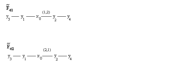
Figure 1.    The diagrams $\widetilde{F}_{41}$ and $\widetilde{F}_{42}$

a) Diagram $\widetilde{F}_{41}$. Here, the Cartan matrix is

$$K=\left(\begin{array}[]{ccccc}2&-1&-2&&\\ -1&2&&-1&\\ -1&&2&&-1\\ &-1&&2&\\ &&-1&&2\\ \end{array}\right)\begin{array}[]{c}x_{0}\\ y_{1}\\ y_{2}\\ y_{3}\\ y_{4}\\ \end{array}$$

The matrix $U$ and the matrix B of the Tits form are as follows:

$$U=\mathop{\mathrm{diag}}\left(\begin{array}[]{c}1\\ 1\\ 1/2\\ 1\\ 1/2\\ \end{array}\right),\qquad{\bf B}=\left(\begin{array}[]{ccccc}2&-1&-2&&\\ -1&2&&-1&\\ -2&&4&&-2\\ &-1&&2&\\ &&-2&&4\\ \end{array}\right).$$

8. The Cartan matrix (example: $\widetilde{F}_{42}$)

b) Diagram $\widetilde{F}_{42}$. The Cartan matrix is

$$K=\left(\begin{array}[]{ccccc}2&-1&-1&&\\ -1&2&&-1&\\ -2&&2&&-1\\ &-1&&2&\\ &&-1&&2\\ \end{array}\right)\begin{array}[]{c}x_{0}\\ y_{1}\\ y_{2}\\ y_{3}\\ y_{4}\\ \end{array},$$

the matrix $U$ and the matrix B of the Tits form are as follows:

$$U=\mathop{\mathrm{diag}}\left(\begin{array}[]{c}1\\ 1\\ 2\\ 1\\ 2\\ \end{array}\right),\qquad{\bf B}=\left(\begin{array}[]{ccccc}2&-1&-1&&\\ -1&2&&-1&\\ -1&&1&&-\displaystyle\frac{1}{2}\\ &-1&&2&\\ &&-\displaystyle\frac{1}{2}&&1\\ \end{array}\right).$$

9. The Cartan matrix and the Coxeter transformation

From (1), (LABEL:matrix_K) we have:

$${\bf C}{z}=\lambda{z}\hskip 8.53581pt\Longleftrightarrow\hskip 8.53581pt\left\{\begin{array}[]{cc}\displaystyle\frac{\lambda+1}{2\lambda}x&=-Dy\\ &\\ \displaystyle\frac{\lambda+1}{2}y&=-Fx\end{array}\right.,\text{ where }z=\left(\begin{array}[]{c}x\\ y\end{array}\right).$$ (4)

$$\left\{\begin{array}[]{c}DD^{t}x=\displaystyle\frac{(\lambda+1)^{2}}{4\lambda}x\vspace{3mm}\\ D^{t}Dy=\displaystyle\frac{(\lambda+1)^{2}}{4\lambda}y\end{array}\right.\hskip 25.60747pt\left\{\begin{array}[]{c}DFx=\displaystyle\frac{(\lambda+1)^{2}}{4\lambda}x\vspace{3mm}\\ FDy=\displaystyle\frac{(\lambda+1)^{2}}{4\lambda}y\end{array}\right.$$ (5)

Proposition 1.

1) The kernel of the matrix B considered as the matrix of an operator acting in the space spanned by roots coincides with the kernel of the Cartan matrix $K$ and coincides with the space of fixed points of the Coxeter transformation

$$\ker{K}=\ker{\bf B}=\{z\mid{\bf C}z=z\}.$$

2) The space of fixed points of the matrix B coincides with the space of anti-fixed points of the Coxeter transformation

$$\{z\mid{\bf B}z=z\}=\{z\mid{\bf C}z=-z\}.$$

10. The eigenvalues of the matrices $DF$ and $FD$

1) The matrices $DF$ and $FD$ have the same non-zero eigenvalues with equal multiplicities.

2) The eigenvalues $\varphi_{i}$ of the matrices $DF$ and $FD$ are non-negative:

$$\varphi_{i}\geq 0.$$

3) The corresponding eigenvalues $\lambda^{\varphi_{i}}_{1,2}$ of the Coxeter transformations are

$$\lambda^{\varphi_{i}}_{1,2}=2\varphi_{i}-1\pm 2\sqrt{\varphi_{i}(\varphi_{i}-1)}.$$ (6)

The eigenvalues $\lambda^{\varphi_{i}}_{1,2}$ either lie on the unit circle or are real positive numbers. It the latter case $\lambda^{\varphi_{i}}_{1}$ and $\lambda^{\varphi_{i}}_{2}$ are mutually inverse:

$$\lambda^{\varphi_{i}}_{1}\lambda^{\varphi_{i}}_{2}=1.$$

11. An example: a simple star $\ast_{k+1}$

In the simply-laced case, the following relation holds:

$$\begin{split}4(D&D^{t})_{ij}=4\sum\limits_{p=1}^{k}{(a_{i},b_{p})(b_{p},a_{j})}=\\ &\begin{cases}s_{i}&\text{if }i=j,\\ 1&\text{if }|v_{i}-v_{j}|=2,\\ 0&\text{if }|v_{i}-v_{j}|>2,\end{cases}\end{split}$$

where $s_{i}$ is the number of edges with the vertex $v_{i}$.

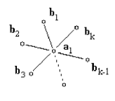
Figure 2.    The star $*_{k+1}$ with $k$ rays

12. An example: a simple star $\ast_{k+1}$ (2)

In the bicolored partition, one part of the graph consists of only one vertex $a_{1}$, i.e., $m=1$, the other one consists of $k$ vertices {$b_{1},\ldots,b_{k}$}. Let $n=k+1$. The $1\times{1}$ matrix $DD^{t}$ is

$$DD^{t}=k=n-1,$$

and the $k\times{k}$ matrix $D^{t}D$ is

$$D^{t}D=\left(\begin{array}[]{ccccc}1&1&1&\dots&1\\ 1&1&1&\dots&1\\ 1&1&1&\dots&1\\ &&&\dots&\\ 1&1&1&\dots&1\end{array}\right).$$

The matrices $DD^{t}$ and $D^{t}D$ have only one non-zero eigenvalue $\varphi_{1}=n-1$. All the other eigenvalues of $D^{t}D$ are zeros and the characteristic polynomial of the $D^{t}D$ is

$$\varphi^{n-1}(\varphi-(n-1)).$$

13. The Perron-Frobenius theorem

Theorem 2.

Let $A$ be an $n\times{n}$ non-negative irreducible matrix. Then the following holds:

1) There exists a positive eigenvalue $\lambda$ such that

$$|\lambda_{i}|\leq\lambda,\text{ where }i=1,2,\dots,n.$$

2) There is a positive eigenvector $z$ corresponding to the eigenvalue $\lambda$:

$$Az=\lambda{z},\text{ where }z=(z_{1},\dots,z_{n})^{t}\text{ and }z_{i}>0\text{ for }i=1,\dots,n.$$

Such an eigenvalue $\lambda$ is called the dominant eigenvalue of $A$.

3) The eigenvalue $\lambda$ is a simple root of the characteristic equation of $A$.

The eigenvalue $\lambda$ is calculated as follows:

$$\begin{split}&\displaystyle\lambda=\max_{z\geq 0}\min_{i}\frac{(Az)_{i}}{z_{i}}\hskip 19.91692pt(z_{i}\neq 0),\\ &\displaystyle\lambda=\min_{z\geq 0}\max_{i}\frac{(Az)_{i}}{z_{i}}\hskip 19.91692pt(z_{i}\neq 0).\end{split}$$

14. The Jordan normal forms of $DF$ and $FD$

Here is an application of the Perron-Frobenius theorem.

The matrices $DD^{t}$ (resp. $D^{t}D$) are symmetric and can be diagonalized in the some orthonormal basis of the eigenvectors from $\mathcal{E}_{\varGamma_{a}}=\mathbb{R}^{h}$ (resp. $\mathcal{E}_{\varGamma_{b}}=\mathbb{R}^{k}$). The Jordan normal forms of these matrices are shown in Fig. 3.

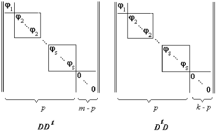
Figure 3.    The Jordan normal forms of $DD^{t}$ and $D^{t}D$

In according to eq. (3.5), (3.14) from [St08], we have:

$$U_{1}A=D,\quad U_{2}A^{t}=F,\quad DF=U_{1}AU_{2}A^{t},$$

where $U_{1}$, $U_{2}$ are positive diagonal matrices, and the eigenvalues of $DF$ and the symmetric matrix

$$\sqrt{U_{1}}{A}U_{2}{A}^{t}\sqrt{U_{1}}$$

coincide.

The normal forms of $DF$ and $FD$ are the same, however, the normal bases (i.e., bases which consist of eigenvectors) for $DF$ and $FD$ are not necessarily orthonormal: $\sqrt{U_{1}}$ does not preserve orthogonality.

15. The eigenvectors of the Coxeter transformation

Case $\varphi_{i}\neq 0,1$:

$$z^{\varphi_{i}}_{r,\nu}=\left(\begin{array}[]{c}\mathbb{X}^{\varphi_{i}}_{r}\vspace{3mm}\\ -\displaystyle\frac{2}{\lambda^{\varphi_{i}}_{\nu}+1}D^{t}\mathbb{X}^{\varphi_{i}}_{r}\end{array}\right),\hskip 11.38109pt1\leq i\leq s,\hskip 5.69054pt1\leq r\leq t_{i},\hskip 5.69054pt\nu=1,2\hskip 2.84526pt.$$

Here $\lambda^{\varphi_{i}}_{1,2}$ is obtained by eq. (6).

Case $\varphi_{i}=1$:

$$z^{1}_{r}=\left(\begin{array}[]{c}\mathbb{X}^{1}_{r}\vspace{3mm}\\ -D^{t}\mathbb{X}^{1}_{r}\end{array}\right),\hskip 11.38109pt\tilde{z}^{1}_{r}=\frac{1}{4}\left(\begin{array}[]{c}\mathbb{X}^{1}_{r}\vspace{3mm}\\ D^{t}\mathbb{X}^{1}_{r}\end{array}\right),\hskip 11.38109pt1\leq r\leq t_{i}.$$

Case $\varphi_{i}=0$:

$$z^{0}_{x_{\eta}}=\left(\begin{array}[]{c}\mathbb{X}^{0}_{\eta}\vspace{3mm}\\ 0\end{array}\right),\hskip 5.69054pt1\leq\eta\leq m-p,\hskip 25.60747ptz^{0}_{y_{\xi}}=\left(\begin{array}[]{c}0\vspace{3mm}\\ \mathbb{Y}^{0}_{\xi}\end{array}\right),\hskip 5.69054pt1\leq\xi\leq k-p.$$

These eigenvectors constitute the basis for the Jordan form of the Coxeter transformation in the simply-laced case. (The multiply-laced case is similarly considered, see §3.2.2 and §3.3.1 from [St08].)

$${\bf C}{z}^{\varphi_{i}}_{r,\nu}=\lambda^{\varphi_{i}}_{1,2}{z}^{\varphi_{i}}_{r,\nu},\qquad\varphi_{i}\neq 0,1.$$

$${\bf C}z^{1}_{r}=z^{1}_{r},\qquad{\bf C}\tilde{z}^{1}_{r}=z^{1}_{r}+\tilde{z}^{1}_{r},\qquad\varphi_{i}=1,\quad\lambda=1.$$

$${\bf C}z^{0}_{x_{\eta}}=-z^{0}_{x_{\eta}},\qquad{\bf C}z^{0}_{y_{\xi}}=-z^{0}_{y_{\xi}},\qquad\varphi_{i}=0,\quad\lambda=-1.$$

16. The Jordan form of the Coxeter transformation

Theorem 3.

1) The Jordan form of the Coxeter transformation is diagonal if and only if the Tits form is non-degenerate.

2) If $\mathcal{B}$ is non-negative definite ($\varGamma$ is an extended Dynkin diagram), then the Jordan form of the Coxeter transformation contains one $2\times 2$ Jordan block. The remaining Jordan blocks are $1\times 1$. All eigenvalues $\lambda_{i}$ lie on the unit circle.

3) If $\mathcal{B}$ is indefinite and degenerate, then the number of $2\times 2$ Jordan blocks coincides with $\dim\ker{\bf B}$. The remaining Jordan blocks are $1\times 1$. There is a simple maximal eigenvalue $\lambda^{\varphi_{1}}_{1}$ and a simple minimal eigenvalue $\lambda^{\varphi_{1}}_{2}$, and

$$\lambda^{\varphi_{1}}_{1}>1,\hskip 14.22636pt\lambda^{\varphi_{1}}_{2}<1.$$

Subbotin-Stekolshchik, [SuSt75], [SuSt78]. Similar results are obtained by A’Campo in [A’C76].

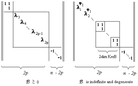
Figure 4.    The Jordan normal form of the Coxeter transformation

17. Example: an arbitrary large number of $2\times 2$ Jordan blocks (Kolmykov)

The example shows that there is a graph $\varGamma$ with indefinite and degenerate quadratic form $\mathcal{B}$ such that $\dim\ker{\bf B}$ is an arbitrarily large number (see Fig. 5) and the Coxeter transformation has an arbitrary large number of $2\times 2$ Jordan blocks.

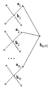
Figure 5.    A graph $\varGamma$ such that $\dim\ker{\bf B}$ is an arbitrary number

We have:

$$4D^{t}D=\left(\begin{array}[]{ccccccc}n&1&1&1&\dots&1&1\\ 1&4&0&0&\dots&0&0\\ 1&0&4&0&\dots&0&0\\ 1&0&0&4&\dots&0&0\\ &&&&\dots&&\\ 1&0&0&0&\dots&4&0\\ 1&0&0&0&\dots&0&4\end{array}\right).$$

It is easy to show that

$$|4D^{t}D-\mu{I}|=(n-\mu)(4-\mu)^{n}-n(4-\mu)^{n-1}.$$

Thus, $\varphi_{i}=\displaystyle\frac{\mu_{i}}{4}=1$ is of multiplicity $n-1$.

18. Monotonicity of the dominant eigenvalue

Proposition 4.

Let us add an edge to a tree $\varGamma$ and let $\stackrel{{\scriptstyle\wedge}}{{\varGamma}}$ be the new graph. Then:

1) The dominant eigenvalue $\varphi_{1}$ may only grow:

$$\varphi_{1}(\stackrel{{\scriptstyle\wedge}}{{\varGamma}})>\varphi_{1}(\varGamma)\hskip 2.84526pt.$$ (7)

2) Let $\varGamma$ be an extended Dynkin diagram, i.e., $\mathcal{B}$ is non-negative definite. Then the spectra of $DD^{t}(\stackrel{{\scriptstyle\wedge}}{{\varGamma}})$ and $D^{t}D(\stackrel{{\scriptstyle\wedge}}{{\varGamma}})$ (resp. $DF(\stackrel{{\scriptstyle\wedge}}{{\varGamma}})$ and $FD(\stackrel{{\scriptstyle\wedge}}{{\varGamma}})$) do not contain $1$, i.e.,

$$\varphi_{i}(\stackrel{{\scriptstyle\wedge}}{{\varGamma}})\neq 1$$

for all $\varphi_{i}$ are eigenvalues of $DD^{t}(\stackrel{{\scriptstyle\wedge}}{{\varGamma}})$.

3) Let $\mathcal{B}$ be indefinite. Then

$$\varphi_{1}(\stackrel{{\scriptstyle\wedge}}{{\varGamma}})>1\hskip 1.42262pt.$$

Subbotin-Stekolshchik, [SuSt75], [SuSt78].

During my talk Ringel noted that (7) is a strict inequality. The strict inequality (7) is, exactly, the result of Th. $1$ from [SuSt78], and it is deduced from the following relation:

$$|DF(\stackrel{{\scriptstyle\wedge}}{{\varGamma}})-\mu{I}|=|DF-\mu{I}|+{\cos}^{2}\{a_{i},b_{s}\}|DF(\stackrel{{\scriptstyle\vee}}{{\varGamma}})-\mu{I}|,$$

where $\stackrel{{\scriptstyle\vee}}{{\varGamma}}$ is the diagram obtained from $\varGamma$ by removing the vertex $a_{i}$, and $b_{s}$ is the new vertex in the diagram $\stackrel{{\scriptstyle\wedge}}{{\varGamma}}$.

19. Theorem on the spectral radius (Ringel)

The spectral radius $\rho(L)$ of a linear transforation $L$ of $\mathbb{R}^{n}$ is the maximum of absolute values of the eigenvalues of $L$. The following theorem (due to C. M. Ringel [Rin94]) concerns the spectral radius of the Coxeter transformation in the case of the generalized Cartan matrix, including the case of diagrams with cycles.

Theorem 5.

Let $A$ be a generalized Cartan matrix which is connected and neither of finite nor of affine type. Let $C$ be a Coxeter transforation for $A$. Then $\rho(C)>1$, and $\rho(C)$ is an eigenvalue of multiplicity one, whereas any other eigenvalue $\lambda$ of $C$ satisfies $|\lambda|<\rho(C)$.

20. The eigenvalues of the affine Coxeter transformation are roots of unity

The Coxeter transformation corresponding to the extended Dynkin diagram is called the affine Coxeter transformation.

Theorem 6.

The eigenvalues of the affine Coxeter transformation are roots of unity.

Subbotin-Stekolshchik [SuSt79], [St82a]. The same theorem for the case of the Dynkin diagrams is due to Coxeter, [Cox51], [Cox49].

The citation from [Cox51]: “Having computed the $m$’s several years earlier [Cox49], I recognized them in the Poincaré polynomials while listening to Chevalley’s address at the International Congress in 1950. I am grateful to A. J. Coleman for drawing my attention to the relevant work of Racah, which helps to explain the “coincidence”; also, to J. S. Frame for many helpful suggestions… ”

In this case: eigenvalues are as follows:

$$\omega^{m_{1}},\quad\omega^{m_{2}},\quad\dots,\quad\omega^{m_{n}},$$

where $\omega=e^{2{\pi}i/h}$, $h$ is the Coxeter number, $m_{i}$ are exponents of eigenvalues, $m_{i}+1$ are the degrees of homogeneous basic elements of $R^{G}$ is the algebra of invariants of the Weyl group $G$.

Let $P(\mathcal{L},t)$ be the Poincaré series of the corresponding Lie group $\mathcal{L}$. Then

$$P(\mathcal{L},t)=(1+t^{2m_{1}+1})(1+t^{2m_{2}+1})\dots(1+t^{2m_{n}+1}).$$

(Hopf’s theorem) [CE48], [Col58], [Sol63].

21. Splitting along the edge formula (Subbotin-Sumin)

An edge $l$ is said to be splitting if by deleting it we split the graph $\varGamma$ into two graphs $\varGamma_{1}$ and $\varGamma_{2}$.

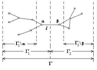
Figure 6.    A split graph $\varGamma$

Proposition 7.

For a given graph $\varGamma$ with a splitting edge $l$, we have

$$\mathcal{X}(\varGamma,\lambda)=\mathcal{X}(\varGamma_{1},\lambda)\mathcal{X}(\varGamma_{2},\lambda)-\lambda\mathcal{X}(\varGamma_{1}\backslash\alpha,\lambda)\mathcal{X}(\varGamma_{2}\backslash\beta,\lambda),$$ (8)

where $\alpha$ and $\beta$ are the endpoints of the deleted edge $l$.

Subbotin-Sumin [SuSum82]. This is the simply-laced case.

22. Splitting along the edge formula (multiply-laced case)

Proposition 8.

For a given graph $\varGamma$ with a splitting weighted edge $l$ corresponding to roots of different lengths, we have

$$\mathcal{X}(\varGamma,\lambda)=\mathcal{X}(\varGamma_{1},\lambda)\mathcal{X}(\varGamma_{2},\lambda)-\rho\lambda\mathcal{X}(\varGamma_{1}\backslash\alpha,\lambda)\mathcal{X}(\varGamma_{2}\backslash\beta,\lambda),$$

where $\alpha$ and $\beta$ are the endpoints of the deleted edge $l$, and $\rho$ is the following factor:

$$\rho=k_{\alpha\beta}k_{\beta\alpha},$$

where $k_{ij}$ is an element of the Cartan matrix, see above examples $\widetilde{F}_{41}$, $\widetilde{F}_{42}$.

Corollary 9.

Let $\varGamma_{2}$ (in Proposition 8) be a component containing a single point. Then, the following formula holds

$$\mathcal{X}(\varGamma,\lambda)=-(\lambda+1)\mathcal{X}(\varGamma_{1},\lambda)-\rho\lambda\mathcal{X}(\varGamma_{1}\backslash\alpha,\lambda),$$

23. Gluing formulas

Proposition 10.

Let $*_{n}$ be a star with $n$ rays coming from the vertex. Let $\varGamma(n)$ be the graph obtained from $*_{n}$ by gluing $n$ copies of the graph $\varGamma$ to the endpoints of its rays . Then

$$\begin{split}&\mathcal{X}(\varGamma(n),\lambda)=\mathcal{X}(\varGamma,\lambda)^{n-1}\varphi_{n-1}(\lambda),\text{ where }\\ &\\ &\varphi_{n}(\lambda)=\mathcal{X}(\varGamma+\beta,\lambda)-n\lambda\mathcal{X}(\varGamma\backslash\alpha,\lambda).\end{split}$$

Subbotin-Sumin [SuSum82]. (See, also §17).

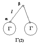
Figure 7.    Splitting along the edge $l$ of the graph $\Gamma(2)$.
Here, the graph $\Gamma(2)$ is obtained by gluing two copies of the graph $\Gamma$.

Proposition 11.

If the spectrum of the Coxeter transformations for graphs $\varGamma_{1}$ and $\varGamma_{2}$ contains an eigenvalue $\lambda$, then this eigenvalue is also the eigenvalue of the Coxeter transformation for the graph $\varGamma$ obtained by gluing as described in Proposition 10.

This proposition follows from the following formula:

$$\begin{split}&\mathcal{X}(\varGamma_{1}+\beta+\varGamma_{2},\lambda)=\\ &\mathcal{X}(\varGamma_{1},\lambda)\mathcal{X}(\varGamma_{2}+\beta,\lambda)-\lambda\mathcal{X}(\varGamma\backslash\alpha,\lambda)\mathcal{X}(\varGamma_{2},\lambda).\end{split}$$

24. The Dynkin diagram ${A}_{n}$, the Frame formula

$$\begin{split}\mathcal{X}({A}_{1})=&-(\lambda+1),\\ \mathcal{X}({A}_{2})=&\lambda^{2}+\lambda+1,\\ \mathcal{X}({A}_{3})=&-(\lambda^{3}+\lambda^{2}+\lambda+1),\\ \mathcal{X}({A}_{4})=&\lambda^{4}+\lambda^{3}+\lambda^{2}+\lambda+1,\\ \dots{\\ }\mathcal{X}({A}_{n})=&-(\lambda+1)\mathcal{X}({A}_{n-1})-\lambda\mathcal{X}({A}_{n-2}),\hskip 14.22636ptn>2.\end{split}$$

J. S. Frame in [Fr51, p.784] obtained that

$$\mathcal{X}({A}_{m+n})=\mathcal{X}({A}_{m})\mathcal{X}({A}_{n})-\lambda\mathcal{X}({A}_{m-1})\mathcal{X}({A}_{n-1}),$$

which easily follows from eq. (8).

25. The spectral radius and Lehmer’s number (McMullen)

Theorem 12.

Either $\rho({\bf C})=1$, or $\rho({\bf C})\geq\lambda_{Lehmer}\approx 1.176281...$ The spectral radius $\rho({\bf C})$ of the Coxeter transformation for all graphs with indefinite Tits form attains its minimum when the diagram is ${E}_{10}$.

(McMullen, [McM02]).

Lehmer’s number is a root $\mathcal{X}(C)$ for the diagram $E_{10}$.

$$\mathcal{X}(C)=x^{10}+x^{9}-x^{7}-x^{6}-x^{5}-x^{4}-x^{3}+x+1,$$

Let $p(x)$ be a monic integer polynomial, and define its Mahler measure to be

$$\|p(x)\|=\prod\limits_{\beta}|\beta|,$$

where $\beta$ runs over all (complex) roots of $p(x)$ outside the unit circle.

In 1933, Lehmer [Leh33] asks whether, for each $\varepsilon\geq 1$, there exists an algebraic integer $\alpha$ such that

$$1<\|\alpha\|<1+\varepsilon.$$ (9)

In [Leh33], Lehmer established that the polynomial with minimal root $\alpha$ (in the sense of (9)) is $E10$. For details, see [Hir02].

26. The spectral radius of diagrams $T_{2,3,n}$ and the Pisot number (Zhang)

The following diagrams belong to the class $T_{2,3,n}$: $D_{5}$ ($n=2$), $E_{6}$ ($n=3$), $E_{7}$ ($n=4$), $E_{8}$ ($n=5$), $\widetilde{E}_{8}$ ($n=6$), $E_{10}$ ($n=7$).

Proposition 13.

The characteristic polynomials of Coxeter transformations for the diagrams $T_{2,3,n}$ are as follows:

$$\mathcal{X}(T_{2,3,n-3})=\lambda^{n}+\lambda^{n-1}-\sum\limits_{i=3}^{n-3}\lambda^{i}+\lambda+1.$$

The spectral radius $\rho(T_{2,3,n-3})$ converges to the maximal root $\rho_{max}$ of the equation

$$\lambda^{3}-\lambda-1=0,$$

and

$$\rho_{max}=\sqrt[3]{\frac{1}{2}+\sqrt{\frac{23}{108}}}+\sqrt[3]{\frac{1}{2}-\sqrt{\frac{23}{108}}}\approx 1.324717...\ .$$

The fact that $\rho(T_{2,3,n})\rightarrow\rho_{max}$ as $n\rightarrow\infty$ was obtained by Zhang [Zh89] and used in the study of regular components of an Auslander-Reiten quiver. The number $\rho_{max}$ coincides with Pisot number.

Recall that an algebraic integer $\lambda>1$ is said to be a Pisot number if all its conjugates (other then $\lambda$ itself) satisfy $|\lambda^{{}^{\prime}}|<1$.

The smallest Pisot number is a root of $\lambda^{3}-\lambda-1=0$ :

$$\lambda_{Pisot}\approx 1.324717...$$

27. The spectral radii of the diagrams $T_{3,3,n}$

Recall that the diagrams $E_{6}$ ($n=2$) and $\widetilde{E}_{6}$ ($n=3$) belong to the class $T_{3,3,n}$.

Proposition 14.

The characteristic polynomials of Coxeter transformations for the diagrams $T_{3,3,n}$ with $n\geq 3$ are as follows:

$$\mathcal{X}(T_{3,3,n})=\lambda^{n+4}+\lambda^{n+3}-2\lambda^{n+1}-3\sum\limits_{i=4}^{n}\lambda^{i}-2\lambda^{3}+\lambda+1,$$

The spectral radius $\rho(T_{3,3,n})$ converges to the maximal root $\rho_{max}$ of the equation

$$\lambda^{2}-\lambda-1=0,$$

and

$$\rho_{max}=\frac{\sqrt{5}+1}{2}\approx 1.618034...\ \text{ (the Golden mean) }.$$

28. The spectral radii of the diagrams $T_{2,4,n}$ (Lakatos)

Recall that the diagrams ${D}_{6}(n=2)$, ${E}_{7}(n=3)$, and $\widetilde{E}_{7}(n=4)$ belong to the class $T_{2,4,n}$.

Proposition 15.

The characteristic polynomials of Coxeter transformations for diagrams $T_{2,4,n}$, where $n\geq 3$, are as follows:

$$\mathcal{X}(T_{2,4,n})=\lambda^{n+4}+\lambda^{n+3}-\lambda^{n+1}-2\sum\limits_{i=4}^{n}\lambda^{i}-\lambda^{3}+\lambda+1,$$

The spectral radius $\rho(T_{2,4,n})$ converges to the maximal root $\rho_{max}$ of the equation

$$\lambda^{3}-\lambda^{2}-1=0,$$

and

$$\rho_{max}=\frac{1}{3}+\sqrt[3]{\frac{58}{108}+\sqrt{\frac{31}{108}}}+\sqrt[3]{\frac{58}{108}-\sqrt{\frac{31}{108}}}\approx 1.465571...\ .$$

Lakatos [Lak99] obtained results on the convergence of the spectral radii $\rho_{max}$ similar to propositions regarding $\rho(T_{2,3,n})$, $\rho(T_{3,3,n})$, $\rho(T_{2,4,n})$.

29. The binary polyhedral groups

We consider the double covering

$$\pi:SU(2)\longrightarrow SO(3,\mathbb{R}).$$

If $G$ is a finite subgroup of $SO(3,\mathbb{R})$, we see that the preimage $\pi^{-1}(G)$ is a finite subgroup of $SU(2)$ and $|\pi^{-1}(G)|=2|G|$. The finite subgroups of $SO(3,\mathbb{R})$ are called polyhedral groups, see Table 1. The finite subgroups of $SU(2)$ are naturally called binary polyhedral groups, see Table 2.

Table 1.   The polyhedral groups in $\mathbb{R}^{3}$

Polyhedron	Orders of symmetries	Rotation group	Group order
Pyramid	$-$	cyclic	$n$
Dihedron	$n$ $2$ $2$	dihedral	$2n$
Tetrahedron	$3$ $2$ $3$	$\mathcal{A}_{4}$	$12$
Cube	$4$ $2$ $3$	$\mathcal{S}_{4}$	$24$
Octahedron	$3$ $2$ $4$	$\mathcal{S}_{4}$	$24$
Dodecahedron	$5$ $2$ $3$	$\mathcal{A}_{5}$	$60$
Icosahedron	$3$ $2$ $5$	$\mathcal{A}_{5}$	$60$

Here, $\mathcal{S}_{m}$ (resp. $\mathcal{A}_{m}$) denotes the symmetric, (resp. alternating)
group of all (resp. of all even) permutations of $m$ letters.

30. The binary polyhedral groups (2)

Table 2.   The finite subgroups of $SU(2)$

$\langle l,m,n\rangle$	Order	Notation	Well-known name
$-$	$n$	$\mathbb{Z}/n\mathbb{Z}$	cyclic group
$\langle 2,2,n\rangle$	$4n$	$\mathcal{D}_{n}$	binary dihedral group
$\langle 2,3,3\rangle$	$24$	$\mathcal{T}$	binary tetrahedral group
$\langle 2,3,4\rangle$	$48$	$\mathcal{O}$	binary octahedral group
$\langle 2,3,5\rangle$	$120$	$\mathcal{J}$	binary icosahedral group

The binary polyhedral group is generated by three generators $R$, $S$, and $T$ subject to the relations

$$R^{p}=S^{q}=T^{r}=RST=-1.$$

Denote this group by $\langle p,q,r\rangle$. The order of the group $\langle p,q,r\rangle$ is

$$\frac{4}{\displaystyle\frac{1}{p}+\frac{1}{q}+\frac{1}{r}-1}.$$

31. The binary polyhedral groups, the algebra of invariants (F. Klein)

Theorem 16.

The algebra of invariants $\mathbb{C}[z_{1},z_{2}]^{G}$ is generated by 3 indeterminates $x,y,z,$ subject to one relation

$$R(x,y,z)=0,$$ (10)

where $R(x,y,z)$ is defined in Table 3. In other words, the algebra of invariants $\mathbb{C}[z_{1},z_{2}]^{G}$ coincides with the coordinate algebra of the curve defined by Eq. (10), i.e.,

$$\mathbb{C}[z_{1},z_{2}]^{G}\simeq\mathbb{C}[x,y,z]/(R(x,y,z)).$$ (11)

F. Klein, 1884, [Kl1884].

Table 3.   The relations $R(x,y,z)$ describing the algebra of invariants $\mathbb{C}[z_{1},z_{2}]^{G}$

Finite subgroup of $SU(2)$	Relation $R(x,y,z)$	Dynkin diagram
$\mathbb{Z}/n\mathbb{Z}$	$x^{n}+yz$	$A_{n-1}$
$\mathcal{D}_{n}$	$x^{n+1}+xy^{2}+z^{2}$	$D_{n+2}$
$\mathcal{T}$	$x^{4}+y^{3}+z^{2}$	$E_{6}$
$\mathcal{O}$	$x^{3}{y}+y^{3}+z^{2}$	$E_{7}$
$\mathcal{J}$	$x^{5}+y^{3}+z^{2}$	$E_{8}$

32. The binary polyhedral groups, Kleinian singularities

The quotient algebra (11) has no singularity except at the origin $O\in\mathbb{C}^{3}$. The quotient variety (or, orbit space) $X=\mathbb{C}^{2}/G$ is isomorphic to (11) (see, [Hob02]).

The quotient variety $X$ is called a Kleinian singularity also known as a Du Val singularity.

33. The binary polyhedral groups, algebras of invariants. An example

Consider the cyclic group $G=\mathbb{Z}/r\mathbb{Z}$ of order $r$. The group $G$ acts on $\mathbb{C}[z_{1},z_{2}]$ as follows:

$$(z_{1},z_{2})\mapsto(\varepsilon{z_{1}},\varepsilon^{r-1}z_{2}),$$

where $\varepsilon=e^{2\pi{i}/r}$, and the polynomials

$$x=z_{1}z_{2},\hskip 14.22636pty=-z_{1}^{r},\hskip 14.22636ptz=z_{2}^{r}$$

are invariant polynomials in $\mathbb{C}[x,y,z]$ which satisfy the following relation

$$x^{r}+yz=0,$$

We have

$$k[V]^{G}=\mathbb{C}[z_{1}z_{2},z_{1}^{r},z_{2}^{r}]\simeq\mathbb{C}[x,y,z]/(x^{r}+yz).$$

34. The binary polyhedral groups,
connection with Dynkin diagrams
(Du Val’s phenomenon)

Du Val obtained the following description of the minimal resolution

$$\pi:\tilde{X}\longrightarrow X$$

of a Kleinian singularity $X=\mathbb{C}^{2}/G$, [DuVal34]

The exceptional divisor (the preimage of the singular point $O$) is a finite union of complex projective lines:

$$\pi^{-1}(O)=L_{1}\cup\dots\cup L_{n},\hskip 8.53581ptL_{i}\simeq\mathbb{CP}^{1}\text{ for }i=1,\dots,n.$$

For $i\neq j$, the intersection $L_{i}\cap L_{j}$ is empty or consists of exactly one point.

To each complex projective line $L_{i}$ (which can be identified with the sphere $S^{2}\subset\mathbb{R}^{3}$) we assign a vertex $i$, and two vertices are connected by an edge if the corresponding projective lines intersect. The corresponding diagrams are Dynkin diagrams, see Table 3.

35. The binary polyhedral groups, Du Val’s phenomenon for binary dihedral group

In the case of the binary dihedral group $\mathcal{D}_{2}$, the real resolution of the real variety

$$\mathbb{C}^{3}/R(x,y,z)\cap\mathbb{R}^{3}$$

gives a rather graphic picture of the complex situation, the minimal resolution $\pi^{-1}:\tilde{X}\longrightarrow X$ for $X=\mathcal{D}_{2}$ is depicted on Fig. 8. Here $\pi^{-1}(O)$ consists of four circles, the corresponding diagram is the Dynkin diagram $D_{4}$.

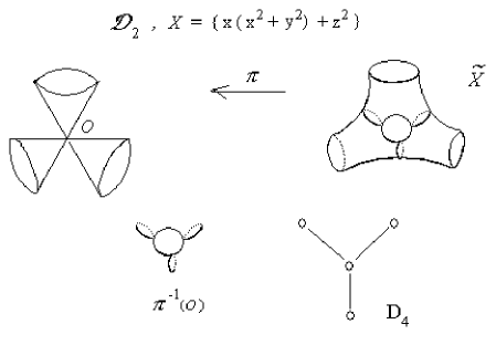
Figure 8.    The minimal resolution $\pi^{-1}:\tilde{X}\longrightarrow X$ for $X=\mathcal{D}_{2}$

36. The McKay correspondence

Let $G$ be a finite subgroup of $SU(2)$. Let $\{\rho_{0},\rho_{1},\dots,\rho_{n}\}$ be the set of all distinct irreducible finite dimensional complex representations of $G$, of which $\rho_{0}$ is the trivial one. Let $\rho:G\longrightarrow SU(2)$ be a faithful representation, then, for each group $G$, we define a matrix $A(G)=(a_{ij})$, by decomposing the tensor products:

$$\rho\otimes\rho_{j}=\bigoplus\limits_{k=0}^{r}a_{jk}\rho_{k},\hskip 19.91692ptj=0,1,...,r,$$ (12)

where $a_{jk}$ is the multiplicity of $\rho_{k}$ in $\rho\otimes\rho_{j}$. McKay observed that

The matrix $2I-A(G)$ is the Cartan matrix of the extended Dynkin diagram $\tilde{\Gamma}(G)$ associated to $G$. There is a one-to-one correspondence between finite subgroups of $SU(2)$ and simply-laced extended Dynkin diagrams.

For the multiply-laced case, the McKay correspondence was extended by D. Happel, U. Preiser, and C. M. Ringel, [HPR80] and by P. Slodowy, [Sl80]. We consider P. Slodowy’s approach.

The systematic proof of the McKay correspondence based on the study of affine Coxeter transformations was given by R. Steinberg, [Stb85].

37. The Slodowy correspondence

Slodowy’s approach is based on the consideration of restricted representations and induced representations instead of an original representation. Let $\rho:G\longrightarrow GL(V)$ be a representation of a group $G$. We denote the restricted representation of $\rho$ to a subgroup $H\subset G$ by $\rho\downarrow^{G}_{H}$, or, briefly, $\rho^{\downarrow}$ for fixed $G$ and $H$. Let $\tau:H\longrightarrow GL(V)$ be a representation of a subgroup $H$. We denote by $\tau\uparrow^{G}_{H}$ the representation induced by $\tau$ to a representation of the group $G$ containing $H$; we briefly write $\tau^{\uparrow}$ for fixed $G$ and $H$.

Let us consider pairs of groups $H\triangleleft G$, where $H$ and $G$ are binary polyhedral groups from Table 4.

Table 4.   The pairs $H\triangleleft G$ of binary polyhedral groups

Subgroup	Dynkin	Group	Dynkin	Index
$H$	diagram	$G$	diagram	$[G:H]$
	$\varGamma(H)$		$\varGamma(G)$
$\mathcal{D}_{2}$	${D}_{4}$	$\mathcal{T}$	${E}_{6}$	$3$
$\mathcal{T}$	${E}_{6}$	$\mathcal{O}$	${E}_{7}$	$2$
$\mathcal{D}_{n-1}$	${D}_{n+1}$	$\mathcal{D}_{2(n-1)}$	${D}_{2n}$	$2$
$\mathbb{Z}/2n\mathbb{Z}$	${A}_{2n-1}$	$\mathcal{D}_{n}$	${D}_{n+2}$	$2$

Let us fix a pair $H\triangleleft G$ from Table 4. We formulate now the essence of the Slodowy correspondence.

38. Induced representations; an example

Let $G$ be a finite group and $H$ any subgroup of $G$. Let $\tau$ be a representation of $H$ in the vector space $V$. The induced representation $\tau\uparrow^{G}_{H}$ of $G$ (or, $\tau^{\uparrow}$, or $\operatorname{Ind}_{H}^{G}\tau$) in the space

$$W=\bigoplus_{x\in G/H}xV$$ (13)

is defined as follows:

$$g\cdot\sum_{x\in G/H}xv_{x}=\sum_{x\in G/H}gxv_{x},$$ (14)

where $v_{x}\in V$ for each $x$.

Example. Let $H$ be a cyclic group of order $3$, $H=\{1,a,a^{2}\}$. Let $\omega:=e^{{2\pi{i}/3}}$. There are $3$ irreducible representations of $H$, or $3$ irreducible $\mathbb{C}H$-submodules of $\mathbb{C}H$:

$$\begin{split}&\tau_{0}=\{1+a+a^{2}\};\quad a*z=z\\ \\ &\tau_{1}=\{1+\omega^{2}{a}+\omega{a^{2}}\};\quad a*z=\omega{z}\\ \\ &\tau_{2}=\{1+\omega{a}+\omega^{2}{a^{2}}\};\quad a*z=\omega^{2}{z}\\ \end{split}$$

and

$$\mathbb{C}H=\tau_{0}\oplus\tau_{1}\oplus\tau_{2}.$$

39. Induced representations; an example (2)

Let $G$ be the rotation group of the triangle

$$\{a,b\mid a^{3}=b^{2}=1,ab=ba^{2}\},$$

The three irreducible right $\mathbb{C}G$-submodules of $\mathbb{C}G$ are as follows:

$$\begin{split}&U_{1}=\{1+a+a^{2}+b+ab+a^{2}{b}\},\\ &\text{ corresponding representation: }\rho_{1}:a\rightarrow 1,b\rightarrow 1,\\ \\ &U_{2}=\{1+a+a^{2}-b-ab-a^{2}{b}\},\\ &\text{ corresponding representation: }\rho_{2}:a\rightarrow 1,b\rightarrow-1,\\ \\ &U_{3}=\{1+\omega^{2}{a}+\omega{a}^{2},\quad b+\omega{b}a+\omega^{2}{b}{a}^{2}\},\\ &U_{4}=\{1+\omega{a}+\omega^{2}{a}^{2},\quad b+\omega^{2}{b}a+\omega{b}{a}^{2}\},\\ &\text{ corresponding representation: }\\ &\rho_{3}:a\rightarrow\left(\begin{array}[]{cc}\omega&0\\ 0&\omega^{2}\\ \end{array}\right),b\rightarrow\left(\begin{array}[]{cc}0&1\\ 1&0\\ \end{array}\right).\\ \\ &\quad\mathbb{C}G=U_{1}\oplus U_{2}\oplus U_{3}\oplus U_{4};\quad U_{3}\simeq U_{4}.\\ \end{split}$$

40. Induced representations; an example (3)

Then, $H\subset G$, elements {$1$, $b$} are two left cosets of $G/H$, and by (13), (14) the induced representations of $G$ are as follows:

$$\begin{split}&\tau_{0}^{\uparrow}=\{1+a+a^{2},\quad b+ab+a^{2}{b}\}=\rho_{1}\oplus\rho_{2},\\ \\ &\tau_{1}^{\uparrow}=\{1+\omega^{2}{a}+\omega{a^{2}},\quad b+\omega^{2}a{b}+\omega{a}^{2}{b}\},\\ \\ &\tau_{2}^{\uparrow}=\{1+\omega{a}+\omega^{2}{a^{2}},\quad b+\omega{a}{b}+\omega^{2}{a}^{2}{b}\},\\ \\ &\tau_{1}^{\uparrow}\simeq\tau_{2}^{\uparrow}\simeq\rho_{3}.\\ \end{split}$$

Here, $b+ab+a^{2}{b}=b+ba^{2}+ba$ , and, equivalently, the right cosets may be considered.

41. The trivial representation, the Frobenius reciprocity

A trivial representation is a representation $(V,\rho)$ of a group $G$ on which all elements of $G$ act as the identity mapping of $V$. The character of the trivial representation is equal to $1$ at any group element.

The Frobenius reciprocity. For characters of restricted representation $\psi^{\downarrow}=\psi\downarrow^{G}_{H}$ and the induced representation $\chi^{\uparrow}=\chi\uparrow^{G}_{H}$, the following relation holds:

$$\langle\psi,\chi^{\uparrow}\rangle_{G}~{}=~{}\langle\psi^{\downarrow},\chi\rangle_{H}.$$ (15)

Let us apply (15) to the trivial representation $\psi$ of $G$. Let $\chi$ be a non-trivial irreducible representation of $H$. Since $\psi^{\downarrow}$ is a trivial representation of $H$, we have $\langle\psi^{\downarrow},\chi\rangle_{H}=0$, and

$$\langle\psi,\chi^{\uparrow}\rangle_{G}=0.$$ (16)

We will use (16) in the proof of the generalized Ebeling theorem, see §51.

42. Restricted representations, Clifford’s theorem

See, [JL01, §20]. In this section, we suppose $H\triangleleft G$.

Theorem 17 (Clifford).

Let $\chi$ be an irreducible character of $G$. Then

(1) all the constituents of $\chi^{\downarrow}_{H}$ have the same degree

(2) if $\psi_{1},\dots,\psi_{m}$ are all the constituents of the $\chi^{\downarrow}_{H}$, then for a positive integer $e$, we have

$$\chi^{\downarrow}_{H}=e(\psi_{1}+...+\psi_{m}).$$

In the following corollary from Clifford’s theorem, we assume that
$[G:H]=2$ (resp. $3$). We are interested in these cases, see Table 4.

Proposition 18.

Let $\chi$ be an irreducible character of $G$. Then either

(1) $\chi^{\downarrow}_{H}$ is irreducible, or

(2) $\chi^{\downarrow}_{H}$ is the sum of $2$ (resp. $3$) distinct irreducible characters of $H$ of the same degree. In this case, we have

$$\chi^{\downarrow}_{H}=\psi_{1}+\psi_{2},\text{ resp. }\chi^{\downarrow}_{H}=\psi_{1}+\psi_{2}+\psi_{3}.\\$$

If $\psi$ is an irreducible character of $G$ such that $\psi^{\downarrow}_{H}$ has $\psi_{1}$ or $\psi_{2}$ (resp., or $\psi_{3}$) as a constituent, then $\psi=\chi$.

Let $\tilde{\pi}$ be the trivial representation of $G$, and let $\chi^{\downarrow}_{H}$ be of case (2) from Prop. 18, and $\tilde{\pi}\neq\chi$. Then $\pi:=\tilde{\pi}^{\downarrow}$ is the trivial representation of $H$, and $\pi$ does not contain $\psi_{i}$ as a constituent, and

$$\langle\pi,\chi^{\downarrow}_{H}\rangle=0.$$ (17)

We will use (17) in the proof of the generalized Ebeling theorem, see §51.

Remark 19.

For case (1) from Prop. 18, there exist non-trivial irreducible representation $\tilde{\pi}\neq\chi$ of $G$, such that $\pi=\chi^{\downarrow}_{H}$. Then, two representations $\pi$ and $\chi^{\downarrow}_{H}$ are gluing on the corresponding folded diagram associated with the Slodowy correspondence, §43, §44.

43. The Slodowy correspondence (2)

1) Let $\rho_{i}$, where $i=1,\dots,n$, be all irreducible representations of $G$; let $\rho^{\downarrow}_{i}$ be the corresponding restricted representations of the subgroup $H$. Let $\rho$ be a faithful representation of $H$, which may be considered as the restriction of a fixed faithful representation $\rho_{f}$ of $G$. Then the following decomposition formula makes sense

$$\rho\otimes\rho^{\downarrow}_{i}=\bigoplus\limits_{j}a_{ji}\rho^{\downarrow}_{j}$$ (18)

and uniquely determines an $n\times{n}$ matrix $\widetilde{A}=(a_{ij})$ such that

$$K=2I-\widetilde{A},$$ (19)

where $K$ is the Cartan matrix of the corresponding folded extended Dynkin diagram.

2) Let $\tau_{i}$, where $i=1,\dots,n$, be all irreducible representations of the subgroup $H$, let $\tau^{\uparrow}_{i}$ be the induced representations of the group $G$. Then the following decomposition formula makes sense

$$\rho\otimes\tau^{\uparrow}_{i}=\bigoplus a_{ij}\tau^{\uparrow}_{j},$$ (20)

i.e., the decomposition of the induced representation is described by the matrix $A^{\vee}=A^{t}$ which satisfies the relation

$$K^{\vee}=2I-\widetilde{A}^{\vee},$$ (21)

where $K^{\vee}$ is the Cartan matrix of the dual folded extended Dynkin diagram.

44. The Slodowy correspondence, folded diagrams

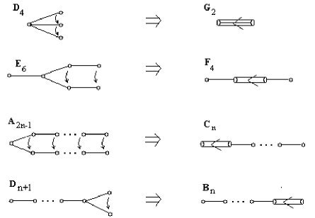
Figure 9.    The folding operation applied to Dynkin diagrams

The folding of Dynkin diagrams is defined by means of the folding of the corresponding Cartan matrices. Let $\tau$ be a diagram automorphism. The folded Cartan matrix $K^{f}$ is defined by taking the sum over all $\tau$-orbits of the columns of $K$ (up to some specific factor of this sum, Mohrdieck, [Mohr04]).

45. The Slodowy correspondence, example: $\mathcal{T}\triangleleft\mathcal{O}$

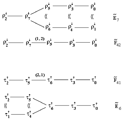
Figure 10.    The induced and restricted representations of $\mathcal{T}\triangleleft\mathcal{O}$

We have

$$\begin{split}&\tau_{3}\otimes\rho_{0}^{\downarrow}=\rho_{3}^{\downarrow}\otimes\rho_{0}^{\downarrow}=\rho_{3}^{\downarrow},\\ &\tau_{3}\otimes\rho_{2}^{\downarrow}=\rho_{3}^{\downarrow}\otimes\rho_{2}^{\downarrow}=\rho_{7}^{\downarrow},\\ &\tau_{3}\otimes\rho_{3}^{\downarrow}=\rho_{3}^{\downarrow}\otimes\rho_{3}^{\downarrow}=\rho_{0}^{\downarrow}+\rho_{5}^{\downarrow},\\ &\tau_{3}\otimes\rho_{5}^{\downarrow}=\rho_{3}^{\downarrow}\otimes\rho_{5}^{\downarrow}=\rho_{3}^{\downarrow}+\rho_{7}^{\downarrow},\\ &\tau_{3}\otimes\rho_{7}^{\downarrow}=\rho_{3}^{\downarrow}\otimes\rho_{7}^{\downarrow}=\rho_{2}^{\downarrow}+2\rho_{5}^{\downarrow},\\ \end{split},\hskip 14.22636pt\widetilde{A}=\left(\begin{array}[]{ccccc}0&1&0&0&0\vspace{2mm}\\ 1&0&2&0&0\vspace{2mm}\\ 0&1&0&1&0\vspace{2mm}\\ 0&0&1&0&1\vspace{2mm}\\ 0&0&0&1&0\end{array}\right)\begin{array}[]{c}\rho_{2}^{\downarrow}\vspace{2mm}\\ \rho_{7}^{\downarrow}\vspace{2mm}\\ \rho_{5}^{\downarrow}\vspace{2mm}\\ \rho_{3}^{\downarrow}\vspace{2mm}\\ \rho_{0}^{\downarrow}\end{array}$$

46. Decomposition $\pi_{n}|_{G}$ (Kostant)

Let $\mathop{\mathrm{Sym}}(\mathbb{C}^{2})$ be the symmetric algebra on $\mathbb{C}^{2}$, in other words, $\mathop{\mathrm{Sym}}(\mathbb{C}^{2})=\mathbb{C}[x_{1},x_{2}]$. The symmetric algebra $\mathop{\mathrm{Sym}}(\mathbb{C}^{2})$ is a graded $\mathbb{C}$-algebra:

$$\mathop{\mathrm{Sym}}(\mathbb{C}^{2})=\mathop{\oplus}\limits_{m=0}^{\infty}{\mathop{\mathrm{Sym}}}^{m}(\mathbb{C}^{2}),$$

where ${\mathop{\mathrm{Sym}}}^{m}(\mathbb{C}^{2})$ denotes the $m$th symmetric power of $\mathbb{C}^{2}$, which consists of the homogeneous polynomials of degree $m$ in $x,y$:

$${\mathop{\mathrm{Sym}}}^{m}(\mathbb{C}^{2})=\text{Span}\{x^{m},x^{m-1}y,\dots,xy^{m-1},y^{m}\}$$

For $n=0,1,2,\dots$, let $\pi_{n}$ be the representation of $SU(2)$ in ${\mathop{\mathrm{Sym}}}^{n}(\mathbb{C}^{2})$ induced by its action on $\mathbb{C}^{2}$. The set {$\pi_{n}\mid n\in\mathbb{Z}_{+}$} is the set of all irreducible representations of $SU(2)$.

Let $G$ be any finite subgroup of $SU(2)$. In [Kos84], Kostant considered the following question:

How does $\pi_{n}|_{G}$ decompose for any $n\in\mathbb{N}$?

In other words: In the decomposition

$$\pi_{n}|_{G}=\sum\limits_{i=0}^{r}{m_{i}(n)\rho_{i}},$$ (22)

where $\rho_{i}$ are irreducible representations of $G$, considered in the context of the McKay correspondence,

What are the multiplicities $m_{i}(n)$ equal to?

47. The Kostant generating function, the multiplicities $m_{i}(n)$

In [Kos84], B. Kostant obtained the multiplicities $m_{i}(n)$ by studying the orbit structure of the Coxeter transformation on the highest root of the corresponding root system.

The multiplicities $m_{i}(n)$ in (22) are calculated as follows:

$$m_{i}(n)=\langle\pi_{n}|G,\rho_{i}\rangle.$$

We extend the relation for multiplicity to the cases of restricted representations $\rho_{i}^{\downarrow}:=\rho_{i}\downarrow_{H}^{G}$ and induced representations $\rho_{i}^{\uparrow}:=\rho_{i}\uparrow_{H}^{G}$, where $H$ is any subgroup of $G$ (in the context of the Slodowy correspondence):

$$m_{i}^{\downarrow}(n)=\langle\pi_{n}|H,\rho_{i}^{\downarrow}\rangle,\hskip 8.53581ptm_{i}^{\uparrow}(n)=\langle\pi_{n}|G,\rho_{i}^{\uparrow}\rangle.$$

Kostant introduced the generating function $P_{G}(t)$ as follows:

$$P_{G}(t)=\left(\begin{array}[]{cc}&[P_{G}(t)]_{0}\vspace{2mm}\\ &\ldots\vspace{2mm}\\ &[P_{G}(t)]_{r}\vspace{2mm}\end{array}\right):=\left(\begin{array}[]{cc}&\sum\limits_{n=0}^{\infty}m_{0}(n){t^{n}}\\ &\ldots\\ &\sum\limits_{n=0}^{\infty}m_{r}(n){t^{n}}\end{array}\right).$$ (23)

We introduce $P_{G\uparrow}(t)$ (resp. $P_{G\downarrow}(t)$) by substituting $m_{i}^{\uparrow}(n)$ (resp. $m_{i}^{\downarrow}(n)$) instead of $m_{i}(n)$.

$$P_{G\uparrow}(t):=\left(\begin{array}[]{cc}&\sum\limits_{n=0}^{\infty}m_{0}^{\uparrow}(n){t^{n}}\\ &\ldots\\ &\sum\limits_{n=0}^{\infty}m_{r}^{\uparrow}(n){t^{n}}\end{array}\right),\quad P_{G\downarrow}(t):=\left(\begin{array}[]{cc}&\sum\limits_{n=0}^{\infty}m_{0}^{\downarrow}(n){t^{n}}\\ &\ldots\\ &\sum\limits_{n=0}^{\infty}m_{r}^{\downarrow}(n){t^{n}}\end{array}\right).$$ (24)

48. The Poincaré series for the binary polyhedral groups

The multiplicity $m_{0}(n)$ corresponds to the trivial representation $\rho_{0}$ in ${\mathop{\mathrm{Sym}}}^{n}(\mathbb{C}^{2})$. The algebra of invariants $R^{G}$ coincides with $\mathop{\mathrm{Sym}}(\mathbb{C}^{2})$, and $[P_{G}(t)]_{0}$ is the Poincaré series of the algebra of invariants $R^{G}=\mathop{\mathrm{Sym}}(\mathbb{C}^{2})^{G}$, i.e., (Kostant, [Kos84])

$$[P_{G}(t)]_{0}=P(\mathop{\mathrm{Sym}}(\mathbb{C}^{2})^{G},t).$$

.

Theorem 20 (Kostant, Knörrer, Gonzalez-Sprinberg, Verdier).

The Poincaré series $[P_{G}(t)]_{0}$ can be calculated as the following rational function:

$$[P_{G}(t)]_{0}=\frac{1+t^{h}}{(1-t^{a})(1-t^{b})},$$

where $h$ is the Coxeter number, while $a$ and $b$ are given by the system

$$a+b=h+2,\quad ab=2|G|.$$

49. The McKay-Slodowy operator

We set

$$v_{n}=\begin{cases}&\sum\limits_{i=0}^{r}{m_{i}(n)}\alpha_{i},\quad\text{ for }B=A,\\ &\sum\limits_{i=0}^{r}{m_{i}^{\downarrow}(n)}\alpha_{i},\quad\text{ for }B=\widetilde{A},\\ &\sum\limits_{i=0}^{r}{m_{i}^{\uparrow}(n)}\alpha_{i},\quad\text{ for }B=\widetilde{A}^{\vee},\\ \end{cases},\quad\rho_{i}=\begin{cases}\rho_{i}\\ \rho_{i}^{\downarrow}\\ \rho_{i}^{\uparrow}\\ \end{cases},\quad m_{i}(n)=\begin{cases}m_{i}(n)\\ m_{i}^{\downarrow}(n)\\ m_{i}^{\uparrow}(n)\\ \end{cases}.$$

The following result of B. Kostant [Kos84], which holds for the McKay operator (12) holds also for the Slodowy operators (18), (20).

Proposition 21.

If $B$ is either the McKay operator $A$ or one of the Slodowy operators $\widetilde{A}$ or $\widetilde{A}^{\vee}$, then

$$Bv_{n}=v_{n-1}+v_{n+1}.$$ (25)

Proof. We have

$$Bv_{n}=B\left(\begin{array}[]{c}m_{0}(n)\\ \dots\\ m_{r}(n)\end{array}\right)=\left(\begin{array}[]{c}\sum a_{0i}\langle\rho_{i},\pi_{n}\rangle\\ \dots\\ \sum a_{ri}\langle\rho_{i},\pi_{n}\rangle\\ \end{array}\right)=\left(\begin{array}[]{c}\langle\rho\otimes\rho_{0},\pi_{n}\rangle\\ \dots\\ \langle\rho\otimes\rho_{r},\pi_{n}\rangle\\ \end{array}\right),$$

where $\rho$ is the irreducible $2D$ representation which coincides with the representation $\pi_{1}$ in ${\mathop{\mathrm{Sym}}}^{2}(\mathbb{C}^{2})$. For representations $\rho_{i}$ of any finite subgroup $G\subset SU(2)$, we have $\langle\chi_{i}\chi_{j},\chi_{k}\rangle~{}=~{}\langle\chi_{i},\chi_{j}\chi_{k}\rangle$, and

$$Bv_{n}=\left(\begin{array}[]{c}\langle\pi_{1}\otimes\rho_{0},\pi_{n}\rangle\\ \dots\\ \langle\pi_{1}\otimes\rho_{r},\pi_{n}\rangle\\ \end{array}\right)=\left(\begin{array}[]{c}\langle\rho_{0},\pi_{1}\otimes\pi_{n}\rangle\\ \dots\\ \langle\rho_{r},\pi_{1}\otimes\pi_{n}\rangle\\ \end{array}\right).$$

By Clebsch-Gordan formula we have

$$\pi_{1}\otimes\pi_{n}=\pi_{n-1}\oplus\pi_{n+1},$$

where $\pi_{-1}$ is the zero representation. ∎

50. The McKay-Slodowy operator (2)

Let $x=\widetilde{P}_{G}(t)$ be given by (23), (24), namely:

$$\widetilde{P}_{G}(t)=\begin{cases}&P_{G}(t)\hskip 8.53581pt\text{ for }B=A,\\ &\\ &P_{G\downarrow}(t)\hskip 5.69054pt\text{ for }B=\widetilde{A},\\ &\\ &P_{G\uparrow}(t)\hskip 5.69054pt\text{ for }B=\widetilde{A}^{\vee},\\ \end{cases}$$ (26)

Proposition 22.

We have

$$tBx=(1+t^{2})x-v_{0},$$ (27)

where $B$ is either the McKay operator $A$ or one of the Slodowy operators $\widetilde{A}$, $\widetilde{A}^{\vee}$.

Proof. From (25) we obtain

$$\begin{split}Bx=&\sum\limits_{n=0}^{\infty}Bv_{n}{t^{n}}=\sum\limits_{n=0}^{\infty}(v_{n-1}+v_{n+1}){t^{n}}=\\ &\sum\limits_{n=0}^{\infty}v_{n-1}t^{n}+\sum\limits_{n=0}^{\infty}v_{n+1}t^{n}=\\ &t\sum\limits_{n=1}^{\infty}v_{n-1}t^{n-1}+t^{-1}\sum\limits_{n=0}^{\infty}v_{n+1}t^{n+1}=\\ &tx+t^{-1}(\sum\limits_{n=0}^{\infty}v_{n}{t^{n}}-v_{0})=tx+t^{-1}x-t^{-1}v_{0}.\qed\end{split}$$

51. The Ebeling theorem

W. Ebeling in [Ebl02] established the connection between the Poincaré series, the Coxeter transformation C, and the corresponding affine Coxeter transformation ${\bf C}_{a}$ (in the context of the McKay correspondence).

Theorem 23.

Let $G$ be a binary polyhedral group and let $[{P}_{G}(t)]_{0}$ be the Poincaré series. Then

$$[{P}_{G}(t)]_{0}=\frac{\det{M_{0}}(t)}{\det{M}(t)},$$

where

$$\det{M}(t)=\det|t^{2}I-{\bf C}_{a}|,\hskip 14.22636pt\det{M_{0}}(t)=\det|t^{2}I-{\bf C}|,$$

C is the Coxeter transformation and ${\bf C}_{a}$ is the corresponding affine Coxeter transformation.

We extend this fact to the case of multiply-laced diagrams, and generalized Poincaré series $[\widetilde{P}_{G}(t)]_{0}$ (in the context of the McKay-Slodowy correspondence), namely:

$$[\widetilde{P}_{G}(t)]_{0}=\frac{\det{M_{0}}(t)}{\det{M}(t)},$$ (28)

see (26).

52. The Ebeling theorem (2)

Proof of (28). From (27) we have

$$[(1+t^{2})I-tB]x=v_{0},$$

where $x$ is the vector $\widetilde{P}_{G}(t)$ and by Cramer’s rule the first coordinate of $\widetilde{P}_{G}(t)$ is

$$[\widetilde{P}_{G}(t)]_{0}=\frac{\det{M_{0}}(t)}{\det{M}(t)},$$

where

$$\det{M}(t)=\det\left((1+t^{2})I-tB\right),$$

and $M_{0}(t)$ is the matrix obtained by replacing the first column of $M(t)$ by $v_{0}=(1,0,...,0)^{t}$. The vector $v_{0}$ corresponds to the trivial representation $\pi_{0}$, and by the McKay-Slodowy correspondence, $v_{0}$ corresponds to the particular vertex which extends the Dynkin diagram to the extended Dynkin diagram. (For calculation of $v_{0}$, see (16), (17), and Remark 19). Therefore, if $\det{M}(t)$ corresponds to the affine Coxeter transformation, and

$$\det{M}(t)=\det|t^{2}I-{\bf C}_{a}|,$$ (29)

then $\det{M_{0}}(t)$ corresponds to the Coxeter transformation, and

$$\det{M_{0}}(t)=\det|t^{2}I-{\bf C}|.$$

So, it suffices to prove (29), i.e.,

$$\det[(1+t^{2})I-tB]=\det|t^{2}I-{\bf C}_{a}|.$$ (30)

53. The Ebeling theorem (3)

If $B$ is the McKay operator $A$ given by (12), then

$$B=2I-K=\left(\begin{array}[]{cc}0&-2D\\ -2D^{t}&0\end{array}\right),$$

where $K$ is a symmetric Cartan matrix (2). If $B$ is the Slodowy operator $\widetilde{A}$ or $\widetilde{A}^{\vee}$ given by (19), (21), then

$$B=2I-K=\left(\begin{array}[]{cc}0&-2D\\ -2F&0\end{array}\right),$$

where $K$ is the symmetrizable Cartan matrix (LABEL:matrix_K). Thus, in the generic case

$$M(t)=(1+t^{2})I-tB=\left(\begin{array}[]{cc}1+t^{2}&2tD\\ 2tF&1+t^{2}\end{array}\right).$$ (31)

Assuming $t\neq 0$ we deduce from (31) that

$$\begin{array}[]{cc}M(t)\left(\begin{array}[]{c}x\\ y\end{array}\right)=0&\Longleftrightarrow\left\{\begin{array}[]{c}(1+t^{2})x=-2tDy,\\ 2tFx=-(1+t^{2})y.\end{array}\right.\vspace{5mm}\\ &\Longleftrightarrow\left\{\begin{array}[]{c}\displaystyle\frac{(1+t^{2})^{2}}{4t^{2}}x=FDy,\vspace{3mm}\\ \displaystyle\frac{(1+t^{2})^{2}}{4t^{2}}y=DFy.\end{array}\right.\end{array}$$ (32)

According to (5), and the propositions about Jordan normal form of the Coxeter transformation, we see that $t^{2}$ is an eigenvalue of the affine Coxeter transformation ${\bf C}_{a}$, i.e., (30) together with (29) are proved. ∎

For further details and references, see [St08]. For applications to the singularity theory, see [Ebl08].

54. Proportionality of characteristic polynomials and folding

By calculating, we obtain that Poincaré series coincide for the following pairs of diagrams

$$\begin{array}[]{cc}{D}_{4}\text{ and }{G}_{2},&{E}_{6}\text{ and }{F}_{4},\\ {D}_{n+1}\text{ and }{B}_{n}(n\geq 4),&{A}_{2n-1}\text{ and }{C}_{n}.\end{array}$$

Note that the second elements of the pairs are obtained by folding:

$$\frac{\mathcal{X}({D}_{4})}{{\mathcal{X}(\widetilde{D}_{4})}}=\frac{\mathcal{X}({G}_{2})}{{\mathcal{X}(\widetilde{G}_{21})}}=\frac{\lambda^{3}+1}{(\lambda^{2}-1)^{2}}.$$

$$\frac{\mathcal{X}({E}_{6})}{{\mathcal{X}(\widetilde{E}_{6})}}=\frac{\mathcal{X}({F}_{4})}{{\mathcal{X}(\widetilde{F}_{41})}}=\frac{\lambda^{6}+1}{(\lambda^{4}-1)(\lambda^{3}-1)}.$$

$$\frac{\mathcal{X}({D}_{n+1})}{{\mathcal{X}(\widetilde{D}_{n+1})}}=\frac{\mathcal{X}({B}_{n})}{{\mathcal{X}(\widetilde{B}_{n})}}=\frac{\lambda^{n}+1}{(\lambda^{n-1}-1)(\lambda^{2}-1)}.$$

$$\frac{\mathcal{X}({A}_{2n-1})}{{\mathcal{X}(\widetilde{A}_{2n-1})}}=\frac{\mathcal{X}({C}_{n})}{{\mathcal{X}(\widetilde{C}_{n})}}=\frac{\lambda^{n}+1}{(\lambda^{n}-1)(\lambda-1)}.$$

55. Acknowledgements

I would like to thank the organizers of the Workshop Jose Antonio de la Pena, Vlastimil Dlab, and Helmut Lenzing who gave me the opportunity to present this survey.

I am thankful to John McKay and Dimitry Leites for helpful comments to this survey.

References

- [A’C76] N. A’Campo, Sur les valeurs propres de la transformation de Coxeter. Invent. Math. 33 (1976), no. 1, 61–67.
- [CE48] C. Chevalley, S. Eilenberg, Cohomology Theory of Lie Groups and Lie Algebras, Transactions of the American Mathematical Society, Vol. 63, No. 1, (Jan., 1948), pp. 85–124.
- [Ch55] C. Chevalley, Invariants of finite groups generated by reflections. Amer. J. Math. 77 (1955), 778–782.
- [Col58] A. J. Coleman, The Betti numbers of the simple Lie groups. Canad. J. Math. 10 (1958), 349–356.
- [Cox34] H. S. M. Coxeter, Discrete groups generated by reflections. Ann. of Math. (2) 35 (1934), no. 3, 588–621.
- [Cox49] H. S. M. Coxeter, Regular polytopes. New York (1949).
- [Cox51] H. S. M. Coxeter, The product of the generators of a finite group generated by reflections. Duke Math. J. 18, (1951), 765–782.
- [JL01] G. James, M. Liebeck, Representations and characters of groups. Second edition. Cambridge University Press, New York, 2001. viii+458 pp. ISBN: 0-521-00392-X.
- [DL03] V. Dlab, P. Lakatos, On spectral radii of Coxeter transformations. Special issue on linear algebra methods in representation theory. Linear Algebra Appl. 365 (2003), 143–153.
- [DrK04] Yu. A. Drozd, E. Kubichka, Dimensions of finite type for representations of partially ordered sets. (English. English summary) Algebra Discrete Math. 2004, no. 3, 21–37.
- [DuVal34] P. Du Val, On isolated singularities which do not affect the condition of adjunction. Proc. Cambridge Phil. Soc. 30 (1934), 453–465.
- [Ebl02] W. Ebeling, Poincaré series and monodromy of a two-dimensional quasihomogeneous hypersurface singularity. Manuscripta Math. 107 (2002), no. 3, 271–282.
- [Ebl08] W. Ebeling, Poincaré series and monodromy of the simple and unimodal boundary singularities. arXiv: 0807.4839, 2008
- [Fr51] J. S. Frame, Characteristic vectors for a product of reflections. Duke Math. J. 18, (1951), 783–785.
- [Hir02] E. Hironaka, Lehmer’s problem, McKay’s correspondence, and . Topics in algebraic and noncommutative geometry (Luminy/Annapolis, MD, 2001), 123–138, Contemp. Math., 324, Amer. Math. Soc., Providence, RI, 2003.
- [Hob02] J. van Hoboken, Platonic solids, binary polyhedral groups, Kleinian singularities and Lie algebras of type . Master’s Thesis, University of Amsterdam, http://home.student.uva.nl/joris.vanhoboken/scriptiejoris.ps, 2002.
- [HPR80] D. Happel, U. Preiser, C. M. Ringel, Binary polyhedral groups and Euclidean diagrams. Manuscripta Math. 31 (1980), no. 1-3, 317–329.
- [Kac80] V. Kac, Infinite root systems, representations of graphs and invariant theory. Invent. Math. 56 (1980), no. 1, 57–92
- [Kl1884] F. Klein, Lectures on the Ikosahedron and the Solution of Equations of the Fifth Degree. Birkhäuser publishing house Basel, 1993 (reproduction of the book of 1888).
- [Kos59] B. Kostant, The principal three-dimensional subgroup and the Betti numbers of a complex simple Lie group. Amer. J. Math. 81 (1959) 973–1032.
- [Kos84] B. Kostant, The McKay correspondence, the Coxeter element and representation theory. The mathematical heritage of Elie Cartan (Lyon, 1984), Asterisque 1985, Numero Hors Serie, 209–255.
- [Lak99] P. Lakatos, On the Coxeter polynomials of wild stars. Linear Algebra Appl. 293 (1999), no. 1-3, 159–170.
- [Leh33] D. H. Lehmer, Factorization of certain cyclotomic functions. Ann. of Math. 34 (1933), 461–469.
- [McM02] C. McMullen, Coxeter groups, Salem numbers and the Hilbert metric. Publ. Math. Inst. Hautes Études Sci. no. 95 (2002), 151–183.
- [Mo68] R. V. Moody, A New Class of Lie Algebras. J. Algebra 10 1968 211–230.
- [Mohr04] S. Mohrdieck A Steinberg Cross-Section for Non-Connected Affine Kac-Moody Groups, 2004, arXiv: math.RT/0401203.
- [Rin94] C. M. Ringel, The spectral radius of the Coxeter transformations for a generalized Cartan matrix. Math. Ann. 300 (1994), no. 2, 331–339.
- [Sol63] L. Solomon, Invariants of finite reflection groups, Nagoya Math. J. Volume 22 (1963), 57-64.
- [Sl80] P. Slodowy, Simple singularities and simple algebraic groups. Lecture Notes in Mathematics, 815. Springer, Berlin, 1980.
- [Stb59] R. Steinberg, Finite reflection groups. Trans. Amer. Math. Soc. 91 (1959), 493–504.
- [Stb85] R. Steinberg, Finite subgroups of , Dynkin diagrams and affine Coxeter elements. Pacific J. Math. 118 (1985), no. 2, 587–598.
- [SuSt75] V. F. Subbotin, R. B. Stekolshchik, The spectrum of the Coxeter transformation and the regularity of representations of graphs. In: Transactions of department of mathematics of Voronezh University. 16, Voronezh Univ. Press, Voronezh (1975), 62–65, (in Russian).
- [SuSt78] V. F. Subbotin, R. B. Stekolshchik, The Jordan form of the Coxeter transformation, and applications to representations of finite graphs. Funkcional. Anal. i Priložen. 12 (1978), no. 1, 84–85. English translation: Functional Anal. Appl. 12 (1978), no. 1, 67–68.
- [SuSt79] V. F. Subbotin, R. B. Stekolshchik, Sufficient conditions of regularity of representations of graphs. Applied analysis, Voronezh, (1979), 105–113, (in Russian).
- [St82a] R. B. Stekolshchik, The Coxeter transformation associated with the extended Dynkin diagrams with multiple edges. Kishinev, VINITI deposition, 02.09.1982, n. 5387-B82, 17p, (in Russian).
- [SuSum82] V. F. Subbotin, M. V. Sumin, Study of polynomials related with graph representations. Voronezh, VINITI deposition, 30.12.1982, n. 6480-B82, 37p, (in Russian).
- [St08] R. Stekolshchik, Notes on Coxeter Transformations and the McKay Correspondence, Springer Monographs in Mathematics, 2008, XX, 240 p.
- [Zh89] Y. Zhang, Eigenvalues of Coxeter transformations and the structure of regular components of an Auslander-Reiten quiver. Comm. Algebra 17 (1989), no. 10, 2347–2362.