On the Bootstrap for
Persistence Diagrams and Landscapes

Abstract

Persistent homology probes topological properties from point clouds and functions. By looking at multiple scales simultaneously, one can record the births and deaths of topological features as the scale varies. In this paper we use a statistical technique, the empirical bootstrap, to separate topological signal from topological noise. In particular, we derive confidence sets for persistence diagrams and confidence bands for persistence landscapes.

Introduction

Persistent homology is a method for studying the homology at multiple scales simultaneously. Given a manifold ${\mathbb{X}}$ embedded in a metric space $\mathbb{Y}$, we consider a probability density function $p\colon\mathbb{Y}\to{\mathbb{R}}$, defined over $\mathbb{Y}$ but concentrated around ${\mathbb{X}}$; that is, the density is positive for a small neighborhood around ${\mathbb{X}}$ and very small over $\mathbb{Y}\,\backslash\,{\mathbb{X}}$. For the right scale parameter $t$, the superlevel set $p^{-1}([t,\infty))$ captures the homology of ${\mathbb{X}}$. The problem, however, is that $t$ is not known a priori. Persistent homology quantifies the topological changes of the superlevel sets with a multiset of points in the extended plane; we call this multiset the persistence diagram, and denote it by $\mathcal{P}$. Another way to represent the information contained in a persistence diagram is with the landscape function $\mathcal{L}\colon{\mathbb{R}}\to{\mathbb{R}}$, which can be thought of as a functional summary of $\mathcal{P}$; we define these concepts in Section 1.1.

Computationally, it may be difficult to compute $\mathcal{P}$ or $\mathcal{L}$ directly. Instead, we assume that $p$ corresponds to a probability distribution $P$, from which we can sample. Given a sample of size $n$, we create an estimate of the probability density function $p_{n}$ using a kernel density estimate. As $n$ increases, $p_{n}$ approaches the true probability density. Given $n$ large enough, we compute the persistence diagram $\mathcal{P}_{n}$ and the landscape $\mathcal{L}_{n}$ corresponding to $p_{n}$.

Sometimes knowing the estimate of a persistence diagram or landscape is not enough. The bigger question is: How close is the estimated persistence diagram or landscape to the true one? We answer this question by constructing a confidence set for persistence diagrams and a confidence band for persistence landscapes.

A $(1-\alpha)$-confidence interval for a parameter $\theta$ is an interval $[a,b]$ such that the probability $\mathbb{P}(\theta\in[a,b])$ is at least $1-\alpha$. In our setting, we desire to find a confidence set for a persistence diagram $\mathcal{P}$. To do so, we compute an estimated diagram $\widehat{\mathcal{P}}$ and and interval $[0,c]$ such that the bottleneck distance between $\mathcal{P}$ and $\widehat{\mathcal{P}}$ is contained in $[0,c]$ with probability $1-\alpha$. That is, we find a metric ball containing $\mathcal{P}$ with high probability.

In this paper, we present the bootstrap, a method for computing confidence intervals, and we apply it to persistence diagrams and landscapes. After briefly reviewing the necessary concepts from computational topology, we give the general technique of bootstrapping in statistics in Section 1.2. In Section 2, we apply the bootstrap to persistence diagrams and landscapes, providing a few examples of these confidence intervals. We conclude in Section 2.3 with a discussion of our ongoing research and open questions.

1 Background

Before presenting our results, we review the necessary definitions and theorems from persistent homology. Then, we present the bootstrap. Due to space constraints, we cover the basics and provide references for a more detailed description.

1.1 Persistence Diagrams and Landscapes

Let ${\mathbb{Y}}$ be a metric space, for example. let ${\mathbb{Y}}$ be a compact subspace of ${\mathbb{R}}^{D}$. Suppose we have a probability density function $p\colon{\mathbb{Y}}\to{\mathbb{R}}$ concentrated in a neighborhood of a manifold ${\mathbb{X}}\subseteq{\mathbb{Y}}$. Persistent homology monitors the evolution of the generators of the homology groups of $p^{-1}([t,\infty))$, the superlevel sets of $p$, and assigns to each generator of these groups a birth time (or scale) $b$ and a death time $d$. The persistence diagram $\mathcal{P}$ records each pair $(b,d)$ as the point $(\frac{b+d}{2},\frac{b-d}{2})$; that is, the $x$-coordinate is the mid-life of the homological feature and the $y$-coordinate is the half-life or half of the persistence of the feature. We refer the reader to Edelsbrunner and Harer (2010) for a more complete introduction to persistent homology.

Let ${\cal D}_{T}$ be the space of positive, countable, $T$-bounded persistence diagrams; that is, for each point $(x,y)=(\frac{b+d}{2},\frac{b-d}{2})\in{\cal P}$, we have $0\leq d\leq b\leq T$ and there are a countable number of points for which $y>0$. We note here that each point on the line $x=0$ is included in the persistence diagram $\mathcal{P}$ with infinite multiplicity. Letting $W_{\infty}(\mathcal{P}_{1},\mathcal{P}_{2})$ denote the bottleneck distance between diagrams $\mathcal{P}_{1}$ and $\mathcal{P}_{2}$, the space $({\cal D},W_{\infty})$ is a metric space. We then have the following stability result from Cohen-Steiner et al. (2007) and generalized in Chazal et al. (2012):

Theorem 1.1 (Stability Theorem).

Let ${\mathbb{M}}$ be finitely triangulable. Let $f,g\colon{\mathbb{M}}\to{\mathbb{R}}$ be two continuous functions. Then, the corresponding persistence diagrams $\mathcal{P}_{f}$ and $\mathcal{P}_{g}$ are well defined, and $W_{\infty}({\cal P}_{f},{\cal P}_{g})\leq\|f-g\|_{\infty}.$

Bubenik (2012) introduced another representation called the persistence landscape, which is in one-to-one correspondence with persistence diagrams. A persistence landscape is a continuous, piecewise linear function $\mathcal{L}\colon{\mathbb{Z}}^{+}\times{\mathbb{R}}\to{\mathbb{R}}$. To define the persistence landscape function, we replace each persistence point $p=(x,y)=\left(\frac{b+d}{2},\frac{b-d}{2}\right)$ with the triangle function

$$t_{p}(z)=\begin{cases}z-x+y&z\in[x-y,x]\\ x+y-z&z\in(x,x+y]\\ 0&\text{otherwise}\end{cases}=\begin{cases}z-d&z\in[d,\frac{b+d}{2}]\\ b-z&z\in(\frac{b+d}{2},b]\\ 0&\text{otherwise}.\end{cases}$$

Notice that $p$ is itself on the graph of $t_{p}(z)$. We obtain an arrangement of curves by overlaying the graphs of the functions $\{t_{p}(z)\}_{p\in\mathcal{P}}$; see Figure 1.

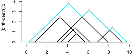
Figure 1: The pink circles are the points in a persistence diagram. The cyan curve is the landscape $\mathcal{L}(1,\cdot)$.

The persistence landscape is defined formally as a walk through this arrangement:

$$\mathcal{L}_{\mathcal{P}}(k,z)=\underset{p\in\mathcal{P}}{\text{kmax}}~{}t_{p}(z),$$ (1)

where kmax is the $k$th maximum value in the set; in particular, $1$max is the usual maximum function. Observe that $\mathcal{L}_{\mathcal{P}}(k,z)$ is $1$-Lipschitz. For the ease of exposition, we will focus on $k=1$ in this paper, using $\mathcal{L}(z)=\mathcal{L}_{\mathcal{P}}(1,z)$. However, the ideas we present in Section 2.2 hold for $k>1$. Our definition of the persistence landscape is equivalent to the original definition given in Bubenik (2012).

1.2 The Standard Bootstrap

Introduced in Efron (1979), the bootstrap is a general method for estimating standard errors and for computing confidence intervals. We focus on the latter in this paper, but refer the interested reader to Efron et al. (2001); Davison and Hinkley (1997), and Van der Vaart (2000) for more details on the versatility of the bootstrap.

Let $X_{1},\dots,X_{n}$ be independent and identically distributed random variables taking values in the measure space $(\mathbb{X},\mathcal{X},P)$. Suppose we are interested in estimating the real-valued parameter $\theta$ corresponding to the distribution $P$ of the observation. We estimate $\theta$ using the statistic $\hat{\theta}=g(X_{1},\dots,X_{n})$, which is some function of the data. For example, $\theta$ and $\hat{\theta}$ could be the population mean and the sample mean, respectively. The distribution of the difference $\hat{\theta}-\theta$ contains all the information that we need to construct a confidence interval of level $1-\alpha$ for $\theta$; that is, an interval $[a,b]$ depending on the data $X_{1},\dots,X_{n}$ such that $\mathbb{P}(\theta\in[a,b])~{}\geq~{}1-\alpha.$ If we knew the cumulative distribution $F$ of $\hat{\theta}-\theta$, then the quantiles $F^{-1}(1-\alpha/2)$ and $F^{-1}(\alpha/2)$ can be computed. Furthermore, setting $a=\hat{\theta}-F^{-1}(1-\alpha/2)$ and $b=\hat{\theta}-F^{-1}(\alpha/2)$, we immediately obtain a $(1-\alpha)$-confidence interval for $\theta$:

$$\mathbb{P}(\theta\in[a,b]) =\mathbb{P}\left(F^{-1}\left(\frac{\alpha}{2}\right)~{}\leq~{}\hat{\theta}-\theta~{}\leq~{}F^{-1}\left(1-\frac{\alpha}{2}\right)\right)=1-\alpha.$$

Unfortunately, the distribution of $\hat{\theta}-\theta$ depends on the unknown distribution $P$.

In the first step in the bootstrap procedure, we approximate the unknown $P$ with the empirical measure $P_{n}$ that puts mass $1/n$ at each $X_{i}$ in the sample. Let $X_{1}^{*},\dots,X_{n}^{*}$ be a sample of size $n$ from $P_{n}$. Equivalently, we can think of drawing $X_{1}^{*},\dots,X_{n}^{*}$ from $X_{1},\dots,X_{n}$ with replacement. We estimate the distribution $F(r)$ with the distribution $\widehat{F}(r)=P_{n}(\hat{\theta}^{*}-\hat{\theta}\leq r)$, where $\hat{\theta}^{*}=g(X_{1}^{*},\dots,X_{n}^{*})$.

The distribution $\widehat{F}$ is still not analytically computable, but can be approximated by simulation: for large $B$, obtain $B$ different values of $\hat{\theta}^{\ast}$ and approximate $\widehat{F}(r)$, and hence $F(r)$, with $\widetilde{F}(r)=\frac{1}{B}\sum_{j=1}^{B}I(\hat{\theta}_{j}^{*}-\hat{\theta}\leq r).$ Since the quantiles of $\widetilde{F}$ approximate the quantiles of $F$, we define the estimated confidence interval as

$$C_{n}=\left[\hat{\theta}-\widetilde{F}_{n}^{-1}(1-\alpha/2)\;,\;\hat{\theta}-\widetilde{F}_{n}^{-1}(\alpha/2)\right].$$ (2)

In summary, the standard bootstrap procedure is:

1. Compute the estimate $\hat{\theta}=g(X_{1},\dots,X_{n})$.

2. Draw $X_{1}^{*},\dots,X_{n}^{*}$ from $P_{n}$ and compute $\hat{\theta}^{*}=g(X_{1}^{*},\dots,X_{n}^{*})$.

3. Repeat the previous step $B$ times to obtain $\hat{\theta}_{1}^{*},\dots,\hat{\theta}_{B}^{*}$.

4. Compute the quantiles of $\widetilde{F}$ and construct the confidence interval $C_{n}$.

There are two sources of error in the Bootstrap procedure. We first approximate $F$ with $\widehat{F}$ and then we estimate $\widehat{F}$ by simulation. The second error can be made arbitrarily small, by choosing $B$ large enough. Therefore, this error is usually ignored in the theory of the bootstrap.
Formally, one has to show that $\sup_{r}\left|\widetilde{F}(r)-F(r)\right|\stackrel{{\scriptstyle P}}{{\to}}0\;,$ which implies that the confidence interval $C_{n}$, defined in (2), is asymptotically consistent at level $1-\alpha$; that is, $\liminf_{n\to\infty}\mathbb{P}(\theta\in C_{n})\geq 1-\alpha.$

1.3 The Bootstrap Empirical Process

When a random variable is a function rather than a real value, the bootstrap procedure described above can be used to construct a confidence interval for the function evaluated at a particular element of the domain. Instead, we use the bootstrap empirical process, which can be used to find a confidence band for a function $h(t)$; that is, we find a pair of functions $a(t)$ and $b(t)$ such that the probability that $h(t)\in[a(t),b(t)]$ for all $t$ is at least $1-\alpha$. We describe this technique below, but refer the reader to Van der Vaart and Wellner (1996) and Kosorok (2008) for more details.

An empirical process is a stochastic process based on a random sample. Let $X_{1},\dots,X_{n}$ be independent and identically distributed random variables taking values in the measure space $(\mathbb{X},\mathcal{X},P)$. For a measurable function $f:\mathbb{X}\to\mathbb{R}$, we denote $Pf=\int fdP$ and $P_{n}f=\int fdP_{n}=n^{-1}\sum_{i=1}^{n}f(X_{i})$. By the law of large numbers $P_{n}f$ converges almost surely to $Pf$. Given a class $\mathcal{F}$ of measurable functions, we define the empirical process $\mathbb{G}_{n}$ indexed by $\mathcal{F}$ as

$$\left\{\mathbb{G}_{n}f\right\}_{f\in\mathcal{F}}=\left\{\sqrt{n}(P_{n}f-Pf)\right\}_{f\in\mathcal{F}}.$$

Example 1.2.

If $\mathcal{F}=\{I(x\leq t)\}_{t\in{\mathbb{R}}}$, then $\{P_{n}f\}_{f\in\mathcal{F}}=\{n^{-1}\sum_{i=1}^{n}I(X_{i}\leq t)\}_{t\in\mathbb{R}}$, which is the empirical distribution function seen as a stochastic process indexed by $t$. Furthermore, we have $\{\mathbb{G}_{n}f\}_{f\in\mathcal{F}}=\{n^{-1/2}\sum_{i=1}^{n}I(X_{i}\leq t)-P(X_{i}\leq t)\}_{t\in\mathbb{R}}$.

Definition 1.3.

A class $\mathcal{F}$ of measurable functions $f:\mathbb{X}\to\mathbb{R}$ is called $P$-Donsker if the process $\{\mathbb{G}_{n}f\}_{f\in\mathcal{F}}$ converges in distribution to a limit process in the space $\ell^{\infty}(\mathcal{F})$, where $\ell^{\infty}(\mathcal{F})$ is the collection of all bounded functions $f:{\mathbb{X}}\to\mathbb{R}$.
The limit process is a Gaussian process $\mathbb{G}$ with zero mean and covariance function $\text{E }\mathbb{G}f\mathbb{G}g:=Pfg-PfPg$; this process is known as a Brownian Bridge.

Let $P_{n}^{*}f=n^{-1}\sum_{i=1}^{n}f(X_{i}^{*})$ where $\{X_{1}^{*},\dots,X_{n}^{*}\}$ is a bootstrap sample from $P_{n}$, the measure that puts mass $1/n$ on each element of the sample $\{X_{1},\dots,X_{n}\}$. The bootstrap empirical process $\mathbb{G}_{n}^{*}$ indexed by $\mathcal{F}$ is defined as

$$\{\mathbb{G}_{n}^{*}f\}_{f\in\mathcal{F}}=\{\sqrt{n}(P_{n}^{*}f-P_{n}f)\}_{f\in\mathcal{F}}.$$

Theorem 1.4 (Theorem 2.4 in Giné and Zinn (1990)).

$\mathcal{F}$ is $P$-Donsker if and only if $\mathbb{G}_{n}^{*}$ converges in distribution to $\mathbb{G}$ in $\ell^{\infty}({\mathcal{F}})$.

In words, Theorem 1.4 states that $\mathcal{F}$ is $P$-Donsker if and only if the bootstrap empirical process converges in distribution to the limit process $\mathbb{G}$ given in Definition 1.3. Suppose we are interested in constructing a confidence band of level $1-\alpha$ for $\{Pf\}_{f\in\mathcal{F}}$, where $\mathcal{F}$ is $P$-Donsker. Let $\hat{\theta}=\sup_{f\in\mathcal{F}}\left|\mathbb{G}_{n}f\right|$. We proceed as follows:

1. Draw $X_{1}^{*},\dots,X_{n}^{*}$ from $P_{n}$ and compute $\hat{\theta}^{*}=\sup_{f\in\mathcal{F}}\left|\mathbb{G}_{n}^{*}f\right|$.

2. Repeat the previous step $B$ times to obtain $\hat{\theta}_{1}^{*},\dots,\hat{\theta}_{B}^{*}$.

3. Compute $q_{\alpha}=\inf\left\{q:\frac{1}{B}\sum_{j=1}^{B}I(\hat{\theta}_{j}^{*}\geq q)\leq\alpha\right\}.$

4. For $f\in\mathcal{F}$ define the confidence band $C_{n}(f)=\left[P_{n}f-\frac{q_{\alpha}}{\sqrt{n}}\,,\,P_{n}f+\frac{q_{\alpha}}{\sqrt{n}}\right].$

A consequence of Theorem 1.4 is that, for large $n$ and $B$, the interval $[0,q_{\alpha}]$ has coverage $1-\alpha$ for $\hat{\theta}$ and the band $C_{n}(f)_{f\in\mathcal{F}}$ has coverage $1-\alpha$ for $\{Pf\}_{f\in\mathcal{F}}$.

2 Applications of the Bootstrap

In this section, we apply the bootstrap from the previous section to persistence diagrams, as well as to persistence landscapes.

2.1 Persistence Diagrams

Let $X_{1},\ldots,X_{n}$ be a sample from the distribution $P$, supported on a smooth manifold $\mathbb{X}\subset\mathbb{R}^{D}$. Let $p_{h}(x)=\int_{\mathbb{X}}\frac{1}{h^{D}}K\left(\frac{||x-u||}{h}\right)dP(u),$ where $K:\mathbb{R}\to\mathbb{R}$ is an integrable function satisfying $\int K(u)du=1$ and $K(u)$ is nonnegative for all $u$; thus $p_{h}$ is a probability distribution. The function $K$ is called a kernel and the parameter $h>0$ is its bandwidth. Then $p_{h}$ is the density of the probability measure $P_{h}$ which is the convolution $P_{h}=P\star\mathbb{K}_{h}$ where $\mathbb{K}_{h}(A)=h^{-D}\mathbb{K}(h^{-1}A)$ and $\mathbb{K}(A)=\int_{A}K(t)dt$. $P_{h}$ is a smoothed version of $P$.

Our target of inference in this section is ${\cal P}_{h}$, the persistence diagram of the superlevel sets of $p_{h}$. The standard estimator for $p_{h}$ is the kernel density estimator

$$\hat{p}_{h}(x)=\frac{1}{n}\sum_{i=1}^{n}\frac{1}{h^{D}}\,K\left(\frac{||x-X_{i}||}{h}\right);$$

notice that if $X_{i}$ are fixed, then $\hat{p}_{h}$ is a porbability distribution. Let $\mathcal{\widehat{P}}_{h}$ be the corresponding persistence diagram. We wish to find a confidence set for $\mathcal{P}_{h}$, i.e. , an interval $[0,c_{n}]$ such that $\limsup_{n\to\infty}\mathbb{P}(W_{\infty}(\mathcal{\widehat{P}}_{h},\mathcal{P}_{h})\in[0,c_{n}])\geq 1-\alpha$. From Theorem 1.1 (Stability), it suffices to find $c_{n}$ such that $\limsup_{n\to\infty}\mathbb{P}(\|\hat{p}_{h}-p_{h}\|_{\infty}>c_{n})\leq\alpha.$

To find $c_{n}$, we use the bootstrap. Let $\mathcal{F}=\left\{f_{x}(u)=\frac{1}{h^{D}}K\left(\frac{\|x-u\|}{h}\right)\right\}_{x\in{\mathbb{X}}}$. Using the notation of Section 1.3, it follows that $Pf_{x}=p_{h}(x)$, $P_{n}f_{x}=\hat{p}_{h}(x)$ and $\hat{\theta}=\sup_{f_{x}\in\mathcal{F}}|\mathbb{G}_{n}f_{x}|=\sqrt{n}\|\hat{p}_{h}-p_{h}\|_{\infty}$. The approximated $1-\alpha$ quantile $q_{\alpha}$ can be obtained through simulation, i.e., $q_{\alpha}=\inf\{q~{}:~{}\frac{1}{B}\sum_{j=1}^{B}I(\sqrt{n}||\hat{p}_{n}^{j}-\hat{p}_{n}||\geq q)\leq\alpha\}$, where $p_{h}^{j}(x)$ denotes the probability distribution corresponding to the $j^{th}$ bootstrap sample. The following result holds under suitable regularity conditions on the kernel $K$ for which $\mathcal{F}$ is Donsker; see Giné and Guillou (2002).

Theorem 2.1 (Lemma 15 in Balakrishnan et al. (2013)).

We have that

$$\;\;\limsup_{n\to\infty}\mathbb{P}\Bigl{(}\sqrt{n}\|\hat{p}_{h}-p_{h}\|_{\infty}>q_{\alpha}\Bigr{)}~{}\leq~{}\alpha.$$

By the Stability Theorem, we conclude: $\;\;\lim_{n\to\infty}\mathbb{P}\left(W_{\infty}(\widehat{\cal P}_{h},{\cal P}_{h})>\frac{q_{\alpha}}{\sqrt{n}}\right)\leq\alpha.$

Example 2.2 (Torus).

We embed the torus $\mathbb{S}^{1}\times\mathbb{S}^{1}$ in ${\mathbb{R}}^{3}$ and we use the rejection sampling algorithm of Diaconis et al. (2012) ($R=1.5,r=0.8$) to sample $10,000$ points uniformly from the torus. Then, we compute the persistence diagram $\mathcal{\widehat{P}}_{h}$ using the Gaussian kernel with bandwidth $h=0.25$ and use the bootstrap to construct the $0.95\%$ confidence interval $[0\,,\,0.01]$ for $W_{\infty}(\mathcal{\widehat{P}}_{h},\mathcal{P}_{h})$; see Figure 2. Notice that the confidence set correctly captures the topology of the torus. That is, only the points representing real features of the torus are significantly far from the horizontal axis.

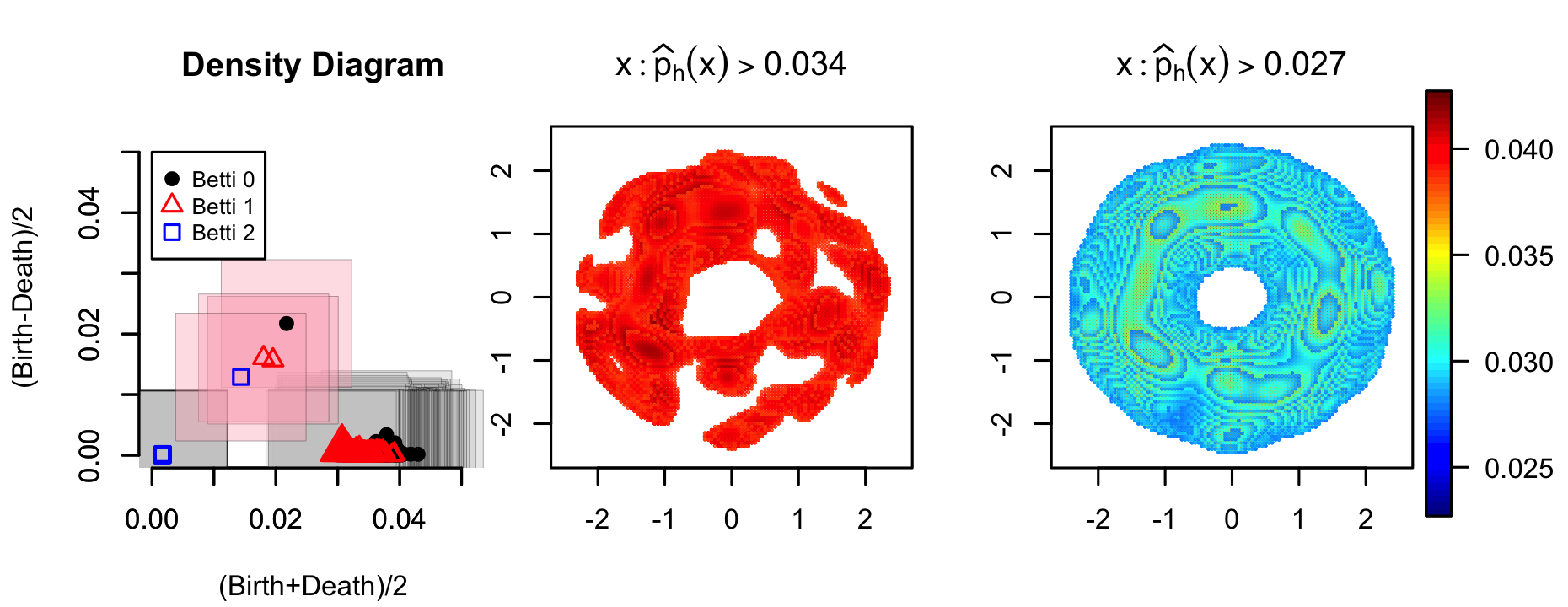
Figure 2: Left: Persistence Diagram of the superlevel sets of a kernel density estimator on the 3D torus described in Example 2.2. The boxes of side $=2\times 0.01$ around the points represent the 95% confidence set for $\mathcal{P}_{h}$. Middle: 2D projection of the superlevel set $\{x:\hat{p}_{h}(x)>0.034\}$. Right: 2D projection of the superlevel set $\{x:\hat{p}_{h}(x)>0.027\}$.

2.2 Landscapes

Let the diagrams $\mathcal{P}_{1},\ldots,\mathcal{P}_{n}$ be a sample from the distribution $P$ over the space of persistence diagrams $\mathcal{D}_{T}$. Thus, by definition, we have $x+y\leq T<\infty$ and $0\leq y\leq T/2$ for all $(x,y)\in\cup_{i}\mathcal{P}_{i}$.

Let $\mathcal{L}_{1},\ldots,\mathcal{L}_{n}$ be the landscape functions corresponding to $\mathcal{P}_{1},\dots,\mathcal{P}_{n}$. That is, $\mathcal{L}_{i}(t)=\mathcal{L}_{\mathcal{P}_{i}}(1,t)$, as defined in (1). We define the mean landscape $\mu(t)=\mathbb{E}_{P}[\mathcal{L}_{i}(t)],$ and the empirical mean landscape $\overline{\cal L}_{n}(t)=\frac{1}{n}\sum_{i=1}^{n}\mathcal{L}_{i}(t).$ In this section, we show that the process $\sqrt{n}(\overline{\cal L}_{n}(t)-\mu(t))$ converges to a Gaussian process, so that we may use the procedure given in Section 1.3.

Let ${\cal F}=\{f_{t}~{}:~{}0\leq t\leq T\}$, where $f_{t}:{\cal D}\to\mathbb{R}$ is defined by $f_{t}(\mathcal{P})=\mathcal{L}_{\mathcal{P}}(1,t)$. We note here that $f_{t}(\mathcal{P})=0$ if $t\notin(0,T)$. We can now write $\sqrt{n}(\overline{\cal L}_{n}(t)-\mu(t))$ as an empirical process indexed by $t\in[0,T]$ :

$$\sqrt{n}(\overline{\cal L}_{n}(t)-\mu(t))=\sqrt{n}\left(\frac{1}{n}\sum_{i=1}^{n}\mathcal{L}_{i}(t)-\mu(t)\right)=\sqrt{n}(P_{n}f_{t}-Pf_{t})\equiv\mathbb{G}_{n}f_{t}.$$

We note that the constant function $F(\mathcal{P})=T/2$ is a measurable envelope for ${\cal F}$.

Given a probability measure $Q$ over $\mathcal{F}$, let $\|f-g\|_{Q,2}=\sqrt{\int|f-g|^{2}dQ}$ and let $N({\cal F},L_{2}(Q),\varepsilon)$ be the covering number of $\mathcal{F}$, that is, the size of the smallest $\varepsilon$-net in this metric.

Lemma 2.3 (Theorem 2.5 in Kosorok (2008)).

Let $\mathcal{F}$ be a class of measurable functions satisfying $\int_{0}^{1}\sqrt{\log\sup_{Q}N(\mathcal{F},L_{2}(Q),\varepsilon\|F\|_{Q,2})}d\varepsilon<\infty\,,$ where $F$ is a measurable envelope of $\mathcal{F}$ and the supremum is taken over all finitely discrete probability measures $Q$ with $\|F\|_{Q,2}>0$. If $PF^{2}<\infty$, then $\mathcal{F}$ is $P$-Donsker.

Theorem 2.4 (Weak Convergence of Landscapes).

Let $\mathbb{G}$ be a Brownian bridge with covariance function $\kappa(t,u)=\int f_{t}(\mathcal{P})f_{u}(\mathcal{P})dP(\mathcal{P})-\int f_{t}(\mathcal{P})dP(\mathcal{P})\int f_{u}(\mathcal{P})dP(\mathcal{P}).$ Then, $\mathbb{G}_{n}$ converges in distribution to $\mathbb{G}.$

Proof.

Since persistence landscapes are $1$-Lipschitz, we have $\|f_{t}-f_{u}\|_{Q,2}\leq|t-u|.$ Construct a regular grid $0\equiv t_{0}<t_{1}<\cdots<t_{N}\equiv T$, where $t_{j+1}-t_{j}=\varepsilon\|F\|_{Q,2}=\varepsilon\,T/2$. We claim that $\{f_{t_{j}}:1\leq j\leq N\}$ is an $(\varepsilon\,T/2)$-net for ${\cal F}$: choose $f_{t}\in\cal F$; then there is a $j$ so that $t_{j}\leq t\leq t_{j+1}$ and $\|f_{t_{j+1}}-f_{t}\|_{Q,2}\leq|t_{j+1}-t|\leq|t_{j+1}-t_{j}|=\varepsilon\,T/2.$ The fact that $\{f_{t_{j}}:1\leq j\leq N\}$ is an $(\varepsilon\,T/2)$-net implies $\sup_{Q}N({\cal F},L_{2}(Q),\varepsilon\|F\|_{Q,2})\leq 2/\varepsilon.$ Hence, $\int_{0}^{1}\sqrt{\log\sup_{Q}N({\cal F},L_{2}(Q),\varepsilon\|F\|_{2})}d\varepsilon<\infty.$ $F={T/2}$ is trivially square-integrable. By Lemma 2.3, $\mathbb{G}_{n}$ converges in distribution to $\mathbb{G}$. ∎

Now that we have shown that $\mathbb{G}_{n}$ converges to a Gaussian process, we can follow the procedure outlined in Section 1.3. Let $P_{n}$ be the empirical measure that puts mass $1/n$ at each diagram $\mathcal{P}_{i}$. We draw $\mathcal{P}_{1}^{\ast},\ldots\mathcal{P}_{n}^{\ast}$ from $P_{n}$ and construct the corresponding landscapes $\mathcal{L}_{1}^{\ast},\dots,\mathcal{L}_{n}^{\ast}$. Let $\mathcal{\overline{L}}_{n}^{*}$ be the empirical mean and $\hat{\theta}^{\ast}=$ $\sup_{t\in{\mathbb{R}}}|\sqrt{n}(\mathcal{\overline{L}}_{n}^{*}(t)-\mathcal{\overline{L}}_{n}(t))|$. Repeating this $B$ times, we obtain $\hat{\theta}_{1}^{\ast},\ldots\hat{\theta}_{B}^{\ast}$, and we compute the quantile $q_{\alpha}$.

Theorem 2.5 (Confidence Band for Persistent Landscapes).

The interval $C_{n}(t)$ indexed by $t\in{\mathbb{R}}$, defined by $C_{n}(t)=\left[\mathcal{\overline{L}}_{n}(t)-\frac{q_{\alpha}}{\sqrt{n}}\;,\;\mathcal{\overline{L}}_{n}(t)+\frac{q_{\alpha}}{\sqrt{n}}\right]$, is a confidence band for $\mu(t)$:

$$\lim_{n\to\infty}\mathbb{P}\left(\mu(t)\in C_{n}(t)\;\text{ for all }t\right)\geq 1-\alpha.$$

Example 2.6 (Circles).

Given the nine circles of radii $0.4$ and $0.3$, shown in Figure 3, we obtain a sample $X_{1},\ldots,X_{100}$ as follows: first, choose a circle $C_{i}$ uniformly at random, then sample a point iid from $C_{i}$. Let $\mathcal{P}$ be the (Betti 1) persistence diagram corresponding to the Rips filtration for the sample, and $\mathcal{L}$ be the landscape corresponding to $\mathcal{P}$. We repeat this $50$ times to obtain diagrams $\mathcal{P}_{1},\ldots\mathcal{P}_{50}$ and landscapes $\mathcal{L}_{1},\ldots\mathcal{L}_{50}$. Then, we use the bootstrap procedure to obtain the quantile $q_{\alpha}=0.234$. Together with $\mathcal{\overline{L}}_{50}$, this gives us an approximated $95\%$ confidence band for $\mu(t)=\mathbb{E}_{P}(\mathcal{L}_{i}(t))$. On the right of Figure 3 we show the empirical mean landscape $\mathcal{\overline{L}}_{50}$ with the $95\%$ confidence band for $\mu(t)$.

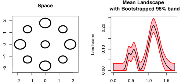
Figure 3: Left: The set of circles from which samples are taken. Right: The confidence band for the persistence landscape corresponding to the distance to the point set.

2.3 Discussion

In this paper, we have described the bootstrap as it applies to persistence diagrams and landscapes. The purpose of this paper was to introduce the bootstrap and the bootstrap empirical process to topologists. In a related paper (Balakrishnan et al. (2013)), aimed towards a statistical audience, we derive the convergence rates for the technique presented in Section 2.1, as well as present three other methods for computing confidence sets for persistence diagrams.

The persistence landscape can be thought of as a summary function of a persistence diagram. The bootstrap method that we presented in Section 2.2 trivially generalizes to handle all landscapes $\mathcal{L}(k,t)$. Furthermore, we need not limit the scope of this method to landscape functions. In a future paper, we plan to investigate other meaningful summary functions as well as the convergence rates for the techniques presented in Section 2.2.

We have demonstrated how the bootstrap works for two examples, given in Figure 2 and Figure 3. Part of our ongoing research is investigating applications for these confidence intervals; in particular, we are applying it to real (rather than simulated) data sets. One can use the confidence intervals for hypothesis testing, but an open question is how to determine the power of such a test.

References

- Balakrishnan et al. [2013] Sivaraman Balakrishnan, Brittany Terese Fasy, Fabrizio Lecci, Alessandro Rinaldo, Aarti Singh, and Larry Wasserman. Statistical inference for persistent homology, 2013. arXiv:1303.7117.
- Bubenik [2012] Peter Bubenik. Statistical topology using persistence landscapes, 2012. arXiv:1207.6437.
- Chazal et al. [2012] Frédéric Chazal, Vin de Silva, Marc Glisse, and Steve Oudot. The structure and stability of persistence modules, July 2012. arXiv:1207.3674.
- Cohen-Steiner et al. [2007] David Cohen-Steiner, Herbert Edelsbrunner, and John Harer. Stability of persistence diagrams. Discrete Comput. Geom., 37(1):103–120, 2007.
- Davison and Hinkley [1997] Anthony Christopher Davison and D. V. Hinkley. Bootstrap Methods and Their Application, volume 1. Cambridge UP, 1997.
- Diaconis et al. [2012] Persi Diaconis, Susan Holmes, and Mehrdad Shahshahani. Sampling from a manifold, 2012. arXiv:1206.6913.
- Edelsbrunner and Harer [2010] Herbert Edelsbrunner and John Harer. Computational Topology. An Introduction. Amer. Math. Soc., Providence, RI, 2010.
- Efron [1979] Bradley Efron. Bootstrap methods: Another look at the jackknife. Ann. Statist. , pages 1–26, 1979.
- Efron et al. [2001] Bradley Efron, Robert Tibshirani, John D. Storey, and Virginia Tusher. Empirical Bayes analysis of a microarray experiment. J. Amer. Statist. Assoc., 96(456):1151–1160, 2001.
- Giné and Guillou [2002] Evarist Giné and Armelle Guillou. Rates of strong uniform consistency for multivariate kernel density estimators. In Annales de l’Institut Henri Poincare (B) Probability and Statistics, volume 38, pages 907–921. Elsevier, 2002.
- Giné and Zinn [1990] Evarist Giné and Joel Zinn. Bootstrapping general empirical measures. The Annals of Probability, pages 851–869, 1990.
- Kosorok [2008] Michael R. Kosorok. Introduction to Empirical Processes and Semiparametric Inference. Springer, 2008.
- Van der Vaart [2000] Aad Van der Vaart. Asymptotic statistics, volume 3. Cambridge university press, 2000.
- Van der Vaart and Wellner [1996] Aad Van der Vaart and Jon Wellner. Weak Convergence and Empirical Processes: With Applications to Statistics. Springer, 1996.