Anomalous D’yakonov-Perel’ spin relaxation in InAs (110) quantum wells under strong magnetic field: role of Hartree-Fock self-energy

Abstract

We investigate the influence of the Hartree-Fock self-energy, acting as an effective magnetic field, on the anomalous D’yakonov-Perel’ spin relaxation in InAs (110) quantum wells when the magnetic field in the Voigt configuration is much stronger than the spin-orbit-coupled field. The transverse and longitudinal spin relaxations are discussed both analytically and numerically. For the transverse configuration, it is found that the spin relaxation is very sensitive to the Hartree-Fock effective magnetic field, which is very different from the conventional D’yakonov-Perel’ spin relaxation. Even an extremely small spin polarization ($P=0.1\%$) can significantly influence the behavior of the spin relaxation. It is further revealed that this comes from the unique form of the effective inhomogeneous broadening, originated from the mutually perpendicular spin-orbit-coupled field and strong magnetic field. It is shown that this effective inhomogeneous broadening is very small and hence very sensitive to the Hartree-Fock field. Moreover, we further find that in the spin polarization dependence, the transverse spin relaxation time decreases with the increase of the spin polarization in the intermediate spin polarization regime, which is also very different from the conventional situation, where the spin relaxation is always suppressed by the Hartree-Fock field. It is revealed that this opposite trends come from the additional spin relaxation channel induced by the HF field. For the longitudinal configuration, we find that the spin relaxation can be either suppressed or enhanced by the Hartree-Fock field if the spin polarization is parallel or antiparallel to the magnetic field.

I Introduction

For the sake of potential spintronic application, the spin dynamics in semiconductor quantum wells (QWs) has been extensively studied in the past decades.review1 ; Bloch ; Awschalom ; Zutic ; fabian565 ; Dyakonov ; wu-review ; Korn ; notebook Among these studies, the spin relaxation is one of the most important problems. In $n$-type semiconductor QWs, it has been understood that the spin relaxation is limited by the D’yakonov-Perel’ (DP) mechanism.DP ; Bloch ; wu-review Very recently, it has been further reported by Zhou et al. that in the framework of the DP mechanism, the spin relaxation time (SRT) $\tau_{s}$ and the momentum relaxation time $\tau_{p}^{\ast}$ show anomalous scalings in InAs (110) QWs under a strong magnetic field ${\bf B}$ in the Voigt configuration satisfying $|g|\mu_{B}B\gg\langle|\Omega_{z}({\bf k})|\rangle$ ($g$ is the effective Landé factor).Zhou There, the effective magnetic field reads ($\hbar\equiv 1$ throughout this paper)Ohno110 ; Wu110 ; Dohrmann04 ; spin_noise110 ; Sherman110 ; Zhou_previous

$${\bf{\Omega}}({\bf{k}})=\big{(}\Omega,0,\gamma_{D}k_{x}(k_{x}^{2}-2k_{y}^{2}-\langle k_{z}^{2}\rangle)/2\big{)},$$ (1)

with $\gamma_{D}$, ${\bf k}=(k_{x},k_{y})$ and $\Omega\equiv g\mu_{B}B$ standing for the Dresselhaus coefficient,dres electron momentum and Zeeman magnetic field, respectively. Due to the unique form of the effective magnetic field, by varying the impurity density, the transverse (longitudinal) spin relaxation can be divided into four (two) regimes: the normal weak scattering regime ($\tau_{\rm s}\propto\tau_{p}^{\ast}$), the anomalous DP-like regime ($\tau_{\rm s}^{-1}\propto\tau_{p}^{\ast}$), the anomalous Elliott-Yafet- (EY-)likeElliott ; Yafet regime ($\tau_{\rm s}\propto\tau_{p}^{\ast}$) and the normal strong scattering regime ($\tau_{\rm s}^{-1}\propto\tau_{p}^{\ast}$) (the anomalous EY-like regime and the normal strong scattering regime).Zhou

In the work of Zhou et al., the spin polarization $P$ is extremely small ($P=0.1\%$ in their work) and the predicted spin relaxations can only be measured by the spin-noise spectroscopy.Sherman4 ; Sherman5 However, this extremely small spin polarization can be hardly resolved by optical orientations, such as the photo-luminescenceBloch ; photoluminescence1 ; photoluminescence2 and Faraday/Kerr measurements.Faraday_Kerr ; Awschalom ; wu-review ; Aws_rotation2 ; Aws_rotation3 ; Korn Therefore, it is essential to study the anomalous DP spin relaxation beyond the extremely small spin polarization. When larger spin polarization is considered, it was theoretically predictedwu-review ; jianhua23 and then experimentally verifiedjianhua36 ; jianhua37 ; jianhua46 that the Hartree-Fock (HF) self-energy, acting as an effective magnetic field,

$${\bf\Omega}_{\rm HF}({\bf k})=-\sum_{{\bf k^{\prime}}}V_{{\bf k-k^{\prime}}}\mbox{Tr}[\rho_{\bf k^{\prime}}\mbox{\boldmath$\sigma$\unboldmath}],$$ (2)

with $V_{{\bf k-k^{\prime}}}$ being the screened Coulomb potential, can efficiently suppress the conventional DP spin relaxation. Similarly, here in the anomalous DP spin relaxation, the HF effective magnetic field is expected to cause rich and intriguing physics. Specifically, by noting that under the strong magnetic field, in the anomalous DP-like regime, the effective inhomogeneous broadening2001 is extremely small (about $0.1\%$ as large as the one in the absence of the strong magnetic field),Zhou even a small spin polarization ($P\approx 0.1\%$ as revealed later) and hence a weak HF effective magnetic field can significantly influence the transverse spin relaxation. This marked suppression of the spin relaxation by the HF magnetic field with such small spin polarization $P\approx 0.1\%$ is beyond expectation and has not yet been reported in the literature.jianhua36 ; jianhua37 ; jianhua46

In the present work, we utilize the kinetic spin Bloch equations (KSBEs) to study the role of the HF effective magnetic field to the anomalous DP spin relaxation in InAs (110) QWs.wu-review With the HF effective magnetic field [Eq. (2)] explicitly included, when $\langle|\Omega_{\rm HF}({\bf k})|\rangle\ll|\Omega|$, the transverse and longitudinal SRTs due to the electron-impurity scattering in the strong scattering limit [$\langle\Omega_{\rm eff}({\bf k})\rangle\tau_{k,2}\ll 1$] become, Yu

$$\tau_{{\rm s}z}^{-1}=\left\langle\Omega^{2}_{\rm eff}({\bf k})\tau_{k,2}+\frac{\overline{{\Omega_{z}({\bf k})}}^{2}\tau_{k,1}}{2(1+\Omega^{2}\tau_{k,1}^{2})}\right\rangle$$ (3)

and

$$\tau_{{\rm s}x}^{-1} = \left\langle\frac{{\overline{\Omega_{z}({\bf k})}}^{2}\tau_{k,1}}{1+[\Omega+\Omega_{\rm HF}({\bf k})]^{2}\tau_{k,1}^{2}}\right\rangle,$$ (4)

respectively, with the effective inhomogeneous broadening being

$$\Omega_{\rm eff}({\bf k})\equiv{|\overline{\Omega^{2}_{z}({\bf k})}|}/(2\Omega\sqrt{1+\Omega^{2}_{\rm HF}({\bf k})\tau_{k,2}^{2}}).$$ (5)

Here, $\overline{A_{\bf k}}=A_{\bf k}-\frac{1}{2\pi}\int d\phi_{\bf k}\,A_{\bf k}$ and the momentum relaxation time $\tau_{k,l}$ limited by the electron-impurity scattering reads

$$\tau_{k,l}^{-1}=\frac{N_{i}}{2\pi}\int_{0}^{2\pi}d\phi_{\bf k-k^{\prime}}|V_{\bf k-k^{\prime}}|^{2}(1-\cos l\phi_{\bf k-k^{\prime}}),$$ (6)

with $N_{i}$ being the impurity density.

These results are consistent with our recent work in the three-dimensional spin-orbit-coupled ultracold Fermi gas, with similar effective magnetic fieldcreated by the Raman beams.Yu ; Wang However, in the two dimensional electron gas (2DEG) system, new features arise due to the k-dependent Coulomb potential, which is different from the contact potential, i.e., constant $V$ in the cold atom system.interaction ; interaction2 ; pwave1 ; Spielman ; Yu With the Coulomb potential, the HF effective magnetic field [Eq. (2)] is also k-dependent and not exactly along the direction of the spin polarization (In the cold atom system, ${\bf\Omega}_{\rm HF}$ is always antiparallel to the spin polarizationYu ). Moreover, in the cold atom system, both the momentum relaxation time ($\tau_{p}^{*}\propto V^{-2}$) and the HF effective magnetic field ($\Omega_{\rm HF}\propto V$) vary simultaneously when tuning the interatom interaction potential by the Feshbach resonance.Feshbach Here, in the 2DEG system, the scattering strength and the HF effective magnetic field can be tuned separately by varying the impurity density and the spin polarization. This provides a platform to study the effects of the scattering and the HF effective magnetic field to the anomalous DP spin relaxation, separately. Furthermore, by noting that in cold atoms, when tuning the interatom interaction potential, $\Omega_{\rm HF}^{2}\tau_{p}^{*}$ is fixed, in the scattering potential dependence, the transverse SRT contributed by the effective inhomogeneous broadening [Eq. (5)] in the anomalous DP-like regime when $|\Omega_{\rm HF}|\tau_{p}^{*}\gg 1$ is independent of the scattering potential. Here, we can utilize the 2DEG system to study the contribution of the effective inhomogeneous broadening in the anomalous DP-like regime to the transverse SRT explicitly.

In this work, we find that for the transverse configuration, the effective inhomogeneous broadening is very small and can be significantly suppressed by the HF field. Hence the spin relaxation is very sensitive to the HF field and even a small spin polarization can significantly influence the transverse spin relaxation. Specifically, with $P=0.1\%$, the normal strong scattering regime in the absence of the HF field vanishes and hence the whole scattering is in the strong scattering limit. Interestingly, a slightly further increase of the spin polarization with $P\gtrsim 1\%$, the transverse SRT is divided into two rather than four regimes: the anomalous EY-like regime and the normal strong scattering regime. Moreover, it is found that in the intermediate spin polarization regime, the HF field can provide an additional spin relaxation channel, and hence the transverse SRT decreases with the increase of the spin polarization. On the other hand, the longitudinal spin relaxation is again divided into the anomalous EY and normal strong scattering regimes in the presence of the HF field. It is further observed that the longitudinal spin relaxation can be either suppressed or enhanced by the HF effective magnetic field if the spin polarization is parallel or antiparallel to the magnetic field.

This paper is organized as follows. In Sec. II, we present the main results. In Sec. II.1, we study the influence of the weak HF effective magnetic field [$\langle|\Omega_{\rm HF}({\bf k})|\rangle\ll|\Omega|$] on the spin relaxation in the impurity density dependence of the SRT with different spin polarizations. We compare the analytical and numerical results in detail with only the electron-impurity scattering. We also discuss the situation with all the relevant scatterings. In Sec. II.2, we study the anomalous spin relaxation under the strong HF effective magnetic field [$\langle|\Omega_{\rm HF}({\bf k})|\rangle>|\Omega|$] and present the spin polarization dependence of the spin relaxation. We summarize in Sec. III.

II Results

The KSBEs are written aswu-review

$$\partial_{t}\rho_{\bf k}(t)=\partial_{t}\rho_{\bf k}(t)|_{\rm coh}+\partial_{t}\rho_{\bf k}(t)|_{\rm scat},$$ (7)

in which $\rho_{\bf k}(t)$ represent the density matrices of electrons with momentum ${\bf k}$ at time $t$. The coherent terms $\partial_{t}\rho_{\bf k}(t)|_{\rm coh}$ describe the spin precessions of electrons due to the effective magnetic field ${\bf\Omega(k)}$ and the HF self-energy. The scattering terms $\partial_{t}\rho_{\bf k}(t)|_{\rm scat}$ include the electron-impurity, electron-electron and electron-phonon scatterings. The expressions for the coherent and scattering terms can be found in Ref. Zhoujun, .

In the numerical calculation, $g=-14.3$ (Ref. g-factor, ) and $\gamma_{D}=-27.3$ eV Å³.Kotani_gamma_D The other material parameters can be found in Ref. Jianhua, . The temperature and the electron density are set to be $T=30$ K and $N_{e}=3\times 10^{11}$ cm^-2, respectively. We further set $B=4$ T, with the condition $|\Omega|\gg\langle|\Omega_{z}({\bf k})|\rangle$ satisfied and the Zeeman splitting energy being much smaller than the Fermi energy. Moreover, the well width is set to be $a=5$ nm, which is much smaller than the cyclotron radius of the lowest Landau level.

With these material parameters, by varying the initial spin polarization and hence the HF effective magnetic field [Eq. (2)], both situations with weak HF effective magnetic field $\langle|\Omega_{\rm HF}({\bf k})|\rangle\ll|\Omega|$ and strong one $\langle|\Omega_{\rm HF}({\bf k})|\rangle\gtrsim|\Omega|$ can be realized. In Secs. II.1 and B, we discuss the spin relaxation with weak HF effective magnetic field $\langle|\Omega_{\rm HF}({\bf k})|\rangle\ll|\Omega|$ and strong one $\langle|\Omega_{\rm HF}({\bf k})|\rangle\gtrsim|\Omega|$, respectively.

II.1 Weak HF effective magnetic field

In this subsection, we discuss the spin relaxation with weak HF effective magnetic field [$\langle|\Omega_{\rm HF}({\bf k})|\rangle\ll|\Omega|$]. In Fig. 1, we plot the transverse and longitudinal SRTs against the impurity density with different initial spin polarizations. Below we first analyze the transverse and longitudinal SRTs with only the electron-impurity scattering and compare the numerical results with the analytical ones; then we discuss the genuine situation with all the relevant scatterings.

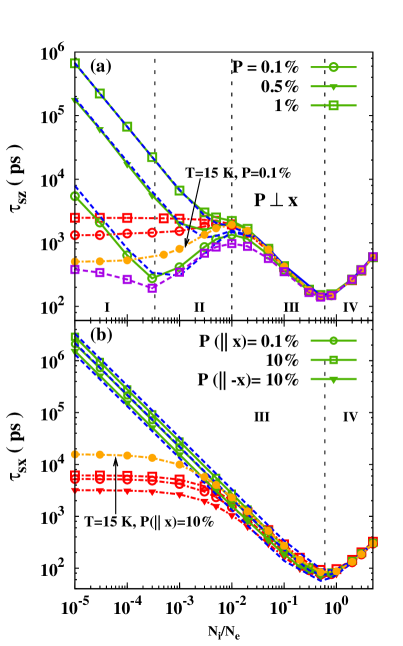
Figure 1: (Color online) Transverse (a) and longitudinal (b) SRTs with only the electron-impurity scattering (green solid curves) and all the relevant scatterings (red chain curves) against the impurity density with different initial spin polarizations. In (a) [(b)], the blue dashed curves represent the analytical results calculated from Eq. (3) [Eq. (4)]. In the calculation, the temperature is set to be 30 K, except for the case plotted by the orange chain curve with dots is calulated at 15 K, representing the transverse (longitudinal) SRT with all the relevant scatterings when $P=0.1\%$ ($10\%$). The purple dashed curve with squares in (a) represents the case with $P=0.1\%$ in the absence of the HF field. The Roman numbers represent different regimes of the spin relaxation: I, the normal weak scattering regime; II, the anomalous DP-like regime; III, the anomalous EY-like regime; IV, the normal strong scattering regime. The vertical black dashed lines indicate the boundaries between different regimes for the transverse (longitudinal) spin relaxation with $P=0.1\%$ in the absence (presence) of the HF field.

II.1.1 Impurity scattering

In this part, we analyze the spin relaxation with only the electron-impurity scattering. With weak HF effective magnetic field [$\langle|\Omega_{\rm HF}({\bf k})|\rangle\ll|\Omega|$], for the transverse (longitudinal) spin relaxation, the HF effective magnetic field acts as a rotating (static) magnetic field around (along) the Zeeman field.Yu In this situation, for the electron-impurity scattering, which is elastic, the transverse (longitudinal) SRT is expressed in Eq. (3) [Eq. (4)]. We first compare the numerical results with the analytical ones from Eqs. (3) and (4). In Fig. 1, the numerical results and the analytical ones are plotted as the green solid and blue dashed curves with different spin polarizations. It is shown that the numerical results agree fairly well with the analytical ones in the whole scattering regime for the transverse [Fig. 1 (a)] and longitudinal [Fig. 1 (b)] SRTs. Accordingly, the underlying physics of the transverse (longitudinal) spin relaxation with weak HF effective magnetic field can be understood facilitated with Eq. (3) [Eq. (4)].

We first analyze the transverse spin relaxation [Fig. 1(a)]. For reference, we present the SRT with the extremely small spin polarization ($P=0.1\%$) in the absence of the HF effective magnetic field (shown by the purple dashed curve with squares). It is shown that the SRTs in this situation can be divided into four regimes: I, the normal weak scattering regime; II, the anomalous DP-like regime; III, the anomalous EY-like regime; IV, the normal strong scattering regime (the boundaries are indicated by the vertical black dashed lines).Zhou When the HF effective magnetic field is included for the situation with $P=0.1\%$ ($0.5\%$), the transverse spin relaxation seemingly can still be divided into four regimes, with the SRT in Regimes I and II enhanced. When the spin polarizations are slightly beyond the extremely small spin polarization ($P=0.1\%$), it is shown in Fig. 1(a) that with $P=1\%$, the SRT is divided into two rather than four regimes. One also observes that with the increase of the initial spin polarization, the anomalous DP-like regime gradually disappears and the SRTs in Regimes I and II are significantly enhanced; whereas the SRTs in Regimes III and IV remain unchanged. These marked influences of such small spin polarizations ($P=0.1\%$ and $1\%$) on the spin relaxation are well beyond expectation [In conventional situation, the effects of the HF effective magnetic field become obvious only when $P\gtrsim 10\%$ (Refs. jianhua36, ; jianhua37, ; jianhua46, )]. Below we show that these intriguing phenomena arise from the suppression of the unique effective inhomogeneous broadening [Eq. (5)] by the HF effective magnetic field.

We begin the analysis from the case with $P=0.1\%$. When the HF effective magnetic field is included, the SRT is still divided into four regimes, but the underlying physics is very different from the case without the HF field. One notes that when $P=0.1\%$, in Regime I (II), $\langle|\Omega_{\rm HF}({\bf k})|\tau_{k,2}\rangle\gtrsim 1$ [$\langle|\Omega_{\rm HF}({\bf k})|\tau_{k,2}\rangle\ll 1$] is satisfied. Accordingly, in Regime I, when $\langle|\Omega_{\rm HF}({\bf k})|\rangle\gtrsim\Omega_{\rm HF}^{c}$ [$\langle|\Omega_{\rm HF}({\bf k})|\rangle\ll\Omega_{\rm HF}^{c}$] with

$$\Omega_{\rm HF}^{c}\equiv\langle|\overline{\Omega^{2}_{z}({\bf k})}|\rangle/{(2|\Omega|)},$$ (8)

$\langle\Omega_{\rm eff}({\bf k})\rangle\tau_{k,2}\approx\langle|\overline{\Omega^{2}_{z}({\bf k})}|/|2\Omega\Omega_{\rm HF}({\bf k})|\rangle$ is smaller (larger) than 1, and hence the normal weak scattering regime is absent (present). By noting that $\Omega_{\rm HF}^{c}$ is extremely small due to the strong Zeeman magnetic field, even with extremely small spin polarization $P=0.1\%$, the HF effective magnetic field can exceed $\Omega_{\rm HF}^{c}$ and the normal weak scattering regime vanishes. That is to say, when $P=0.1\%$, the whole scattering regime is in the strong scattering limit and all the behaviors of the transverse SRT can be analyzed facilitated with Eq. (3).

Specifically, in Rigme I with $\langle|\Omega_{\rm HF}({\bf k})|\tau_{k,2}\rangle\gg 1$, the SRT

$$\tau_{sz}\approx\left\langle 4\Omega^{2}\Omega_{\rm HF}({\bf k})\tau_{k,2}\Big{/}\overline{\Omega_{z}^{2}({\bf k})}^{2}\right\rangle$$ (9)

is proportional to the momentum relaxation time, showing the EY-like behavior (Without the HF effective magnetic field, this behavior is understood due to the spin relaxation channel provided by the momentum relaxation in the weak scattering limitZhou ). In Regime II with $\langle|\Omega_{\rm HF}({\bf k})|\tau_{k,2}\rangle\ll 1$, the SRT is still inversely proportional to the momentum relaxation time, and can be enhanced due to the suppression of the effective inhomogeneous broadening [Eq. (5)] by the HF effective magnetic field. In Regimes III and IV, the SRT is uninfluenced by the HF effective magnetic field. Furthermore, the boundary between Regimes I/II, II/III and III/IV can be determined from Eq. (3). The position of the basin at the crossover between I/II is determined by

$$\tau_{k,2}\approx\langle|\Omega_{\rm HF}({\bf k})|\rangle^{-1},$$ (10)

(instead of $\tau_{k,2}\approx\langle\Omega_{\rm eff}({\bf k})\rangle^{-1}$ in the absence of the HF effective magnetic fieldZhou ); the position of the peak at the crossover between II/III is determined by

$$\tau_{k,1}\tau_{k,2}\approx\left\langle\overline{\Omega_{z}({\bf k})}^{2}\Big{/}[2\Omega^{2}\Omega_{\rm eff}^{2}({\bf k})]\right\rangle;$$ (11)

the basin at the crossover between III/IV is determined by

$$\tau_{k,1}\approx|\Omega|^{-1}.$$ (12)

One notes that from Eq. (10) [Eq. (11)], when the HF effective magnetic field increases, the boundary between Regimes I/II (II/III) is shifted to the stronger (weaker) scattering. Hence with larger spin polarization $P=0.5\%$, the range of Regime II is significantly suppressed. Furthermore, one expects that with the spin polarization, and hence the HF effective magnetic field large enough, Regime II may vanish. This phenomenon arises in our situation with $P=1\%$. When $P=1\%$, in Regimes I and II, by noting that $\langle|\Omega_{\rm HF}({\bf k})|\rangle\tau_{k,2}\gtrsim 1$ is satisfied, the SRT becomes

$$\tau_{{\rm s}z}\approx\left\langle\overline{\Omega^{2}_{z}({\bf k})}^{2}\Big{/}[4\Omega^{2}\Omega^{2}_{\rm HF}({\bf k})\tau_{k,2}]\right\rangle^{-1},$$ (13)

which shows the EY-like behavior. With the original anomalous EY-like and normal strong scattering regimes keeping unchanged, the spin relaxation is divided into two regimes: the anomalous EY-like and normal strong scattering regimes.

It is noted that when $P\lesssim 0.02\%$, the condition $\langle|\Omega_{\rm HF}({\bf k})|\rangle\ll\Omega_{\rm HF}^{c}$ is satisfied, and the normal weak scattering regime still arises. The underlying physics then returns to the one revealed in Ref. Zhou, with the HF effective magnetic field absent.

Although weak HF magnetic field can have marked influence on the transverse spin relaxation, for the longitudinal configuration, the situation is very different. Below we analyze the longitudinal spin relaxation [Fig. 1(b)]. For reference, the SRT with an extremely small spin polarization ($P=0.1\%$) is plotted, which can be divided into two regimes: III, the anomalous EY-like regime and IV, the normal strong scattering regime.Zhou When the spin polarization is large with $P=10\%$, the spin relaxation also presents similar behavior to the situation with small spin polarization, showing a basin with the increase of the impurity density. Furthermore, compared with the situation with $P=0.1\%$, when the initial spin polarization is parallel (antiparallel) to the external magnetic field, the SRT is slightly enhanced (suppressed) in the anomalous EY-like regime and unchanged in the normal strong scattering regime. This is shown by the green solid curve with squares (triangles) in Fig. 1(b) for the spin polarization parallel (antiparallel) to the external magnetic field. These phenomena can be understood as follows.

With the weak HF effective magnetic field, from Eq. (4), we conclude that the longitudinal SRT is divided into two regimes with the boundary determined by

$$\tau_{k,1}=\langle|\Omega+\Omega_{\rm HF}({\bf k})|\rangle^{-1}.$$ (14)

Furthermore, one notes that the HF effective magnetic field is parallel to the spin polarization [Eqs. (2)]. Hence in the anomalous EY-like regime, with $\langle|\Omega_{\rm HF}({\bf k})|\rangle\ll|\Omega|$, when the spin polarization is parallel (antiparallel) to the external magnetic field, the total magnetic field $|\Omega+\Omega_{\rm HF}({\bf k})|$ along the $\hat{x}$-axis is slightly enhanced (suppressed) by the HF effective magnetic field. Accordingly, from Eq. (4), in which $|\Omega+\Omega_{\rm HF}({\bf k})|$ appears in the denominator, the SRT is enhanced (suppressed) in the anomalous EY-like regime. For the spin relaxation in the normal strong scattering regime, with weak HF effective magnetic field [$\langle|\Omega_{\rm HF}({\bf k})|\rangle\ll|\Omega|$], the condition $|\Omega+\Omega_{\rm HF}({\bf k})|\tau_{k,1}\ll 1$ is satisfied and hence the SRT is unchanged by the HF effective magnetic field.

II.1.2 All relevant scatterings

In this part, we discuss the genuine situation with all the relevant scatterings, which are evitable when $T=30$ K, included. The results are plotted as red chain curves in Fig. 1 with different initial spin polarizations [In Fig. 1(a), the case with $P=0.5\%$ is not shown explicitly as it is very close to the case with $P=0.1\%$]. For the transverse spin relaxation [Fig. 1(a)], it is shown that when the electron-electron and electron-phonon scatterings are included, with $P=0.1\%$ ($1\%$), the SRT in Regimes I and II increases (decreases) slowly with increasing impurity density; in Regimes III and IV the SRT remains unchanged. This is because when $T=30$ K, when the impurity density is low (high), the electron-electron (electron-impurity) scattering dominates the momentum relaxation, and hence the SRT with low (high) impurity density is determined by the electron-electron (electron-impurity) scattering. Specifically, in the low impurity density limit, the momentum relaxation time changes little by varying the impurity density, and hence the SRT with $P=0.1\%$ ($1\%$) varies slowly with the increase of the impurity density when $N_{i}\lesssim 0.01N_{e}$. Therefore, to observe the different regimes of spin relaxation in the impurity density dependence clearly, one has to carry out the measurement at low temperature with the electron-electron scattering being suppressed. The situation with lower temperature $T=15$ K is shown Fig. 1(a) by the orange chain curve with all the relevant scatterings when $P=0.1\%$, in which Regime II is clearly revealed.

For the longitudinal spin relaxation [Fig. 1(b)], no matter the spin polarization is small with $P=0.1\%$ or large with $P=10\%$, when the electron-electron and electron-phonon scatterings are included, in the anomalous EY-like regime, the SRT decreases first slowly and then fastly with the increase of the impurity density; in the normal strong scattering regime, the SRT is unchanged. This is understood that the electron-electron (electron-impurity) scattering is dominant in the momentum relaxation when the impurity density is low (high). In Fig. 1 (b), the SRT at 15 K is also plotted by the orange chain curve with all the relevant scatterings when the polarization is parallel to the magnetic field with $P=10\%$.

II.2 Strong HF effective magnetic field

In this subsection, we discuss the spin relaxation with the strong HF effective magnetic field [$\langle|\Omega_{\rm HF}({\bf k})|\rangle\gtrsim|\Omega|$]. In Fig. 2, the transverse and longitudinal SRTs are plotted against the initial spin polarization with different impurity densities $N_{i}=0.003N_{e}$ and $2N_{e}$. One notes that in the absence of the HF effective magnetic field, when $N_{i}=0.003N_{e}$ ($2N_{e}$), the transverse spin relaxation is in the anomalous DP-like (normal strong scattering) regime [Fig. 1(a)]; the longitudinal spin relaxation is in the anomalous EY-like (normal strong scattering) regime [Fig. 1(b)]. Hence with different impurity density, we can discuss spin relaxation in different regimes with the strong HF effective magnetic field by varying the initial spin polarization. Below we first analyze the transverse and longitudinal SRTs with only the electron-impurity scattering, in order to reveal the underlying physics for the anomalous DP relaxation with strong HF effective magnetic field. Then we discuss the genuine situation with all the relevant scatterings.

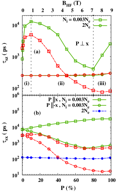
Figure 2: (Color online) Transverse (a) and longitudinal (b) SRTs with only the electron-impurity scattering (green solid curves) and all the relevant scatterings (chain curves) against the initial spin polarization with the different impurity density $N_{i}=0.003N_{e}$ and $2N_{e}$. With $N_{i}=2N_{e}$, the case with ${\bf P}\parallel{\bf\hat{x}}$ is not shown explicitly as it is very close to the one with ${\bf P}\parallel{\bf-\hat{x}}$; the cases with all the relevant scatterings included are not shown either as they coincide with the ones with only the electron-impurity scattering. According to the relative magnitudes of the HF field and the Zeeman field, for the case with $N_{i}=0.003N_{e}$ and only the electron-impurity scattering included, three regimes are shown in (a), separated by the vertical black dashed lines: (i): $\langle|\Omega_{\rm HF}({\bf k})|\rangle\ll|\Omega|$; (ii): $\langle|\Omega_{\rm HF}({\bf k})|\rangle\sim|\Omega|$ and (iii): $\langle|\Omega_{\rm HF}({\bf k})|\rangle\gg|\Omega|$. We also plot the corresponding HF field $B_{\rm HF}$ against the initial spin poalrization (note the scale is on the top frame of the figure).

II.2.1 Impurity scattering

In this part, we analyze the spin relaxation with only the electron-impurity scattering. These results are plotted as green solid curves in Fig. 2. We first analyze the transverse spin relaxation. In Fig. 2(a), when $N_{i}=0.003N_{e}$, it is very interesting to see that the SRT shows a peak and a basin with the increase of the initial spin polarization. Specifically, the suppression of the SRT with the increase of the spin polarization in the intermediate regime is very intriguing and far beyond expectation (In conventional situation, the SRT is always enhanced due to the suppression of the inhomogeneous broadening by the HF fieldjianhua23 ; jianhua36 ; jianhua37 ; jianhua46 ). According to the relative magnitudes of the HF effective magnetic field [$B_{\rm HF}\equiv\langle|\Omega_{\rm HF}({\bf k})/(g\mu_{B})|\rangle$] and the Zeeman magnetic field, we further divide the spin relaxation into three regimes : (i): $\langle|\Omega_{\rm HF}({\bf k})|\rangle\ll|\Omega|$; (ii): $\langle|\Omega_{\rm HF}({\bf k})|\rangle\sim|\Omega|$ and (iii): $\langle|\Omega_{\rm HF}({\bf k})|\rangle\gg|\Omega|$. When $N_{i}=2N_{e}$, the SRT increases slowly with the increase of the initial spin polarization. Below, we analyze the situation with $N_{i}=0.003N_{e}$ and $2N_{e}$, respectively.

For the transverse configuration, when $N_{i}=0.003N_{e}$, we first analyze the spin relaxation in the limit situations with extremely weak [(i)] and strong [(iii)] HF effective magnetic fields, and then focus on the situation with intermediate [(ii)] HF field. In Regime (i), the HF effective magnetic field is extremely weak, and hence acts as a rotating magnetic field around the Zeeman field.Yu The underlying physics has been addressed in Sec. II.1, with the SRT determined by Eq. (3). Accordingly, when the spin relaxation is in the anomalous DP-like regime (when the HF field is absent) with $N_{i}=0.003N_{e}$, the SRT can be significantly enhanced by the HF effective magnetic field.

In Regime (iii), with $\langle|\Omega_{\rm HF}({\bf k})|\rangle\gg|\Omega|$, the HF effective magnetic field acts as a static magnetic field. In this situation, the system returns to the longitudinal configuation as a large static magnetic field, i.e., the large HF effective magnetic field parallel to the spin polarization. Accordingly, from Eq. (4), the SRT is effectively enhanced due to the suppression of the inhomogeneous broadening by this large HF effective magnetic field. Therefore, the SRT increases with the increase of the initial spin polarization.

In Regime (ii), one finds that the HF effective magnetic field is in the intermediate regime between Regimes (i) and (iii). The HF effective magnetic field not only acts as a rotating magnetic field around the Zeeman field, but also plays the role of a static magnetic field. Specifically, when this effective static magnetic field is much smaller than the Zeeman magnetic field, its influence to the transverse spin relaxation can be revealed analytically. In this situation, by noting that there exists a strong magnetic field in the plane of QWs, the in-plane component of this effective static magnetic field can be neglected. Therefore, we keep the $\hat{z}$-component $B_{z}^{\rm HF}$ of the effective static magnetic field in the KSBEs, and obtain the transverse SRT when $\omega_{z}\equiv|g|\mu_{B}B_{z}^{\rm HF}\ll|\Omega|$ (refer to Appendix A),

$$\tau_{sz}^{*-1}=\tau_{sz}^{-1}+\left\langle{\omega_{z}^{2}\overline{\Omega_{z}({\bf k})}^{2}\tau_{k,1}}/{\Omega^{2}}\right\rangle.$$ (15)

Hence the effective static magnetic field provides an additional spin relaxation channel to the transverse spin relaxation. The underlying physics can be understood as follows. Considering the total magnetic field $\Omega_{\rm tot}$ from the Zeeman ($\Omega$) and effective static fields ($\omega_{z}$), when $\omega_{z}\ll|\Omega|$,

$$\Omega_{\rm tot}=\sqrt{\Omega^{2}+\omega_{z}^{2}}\approx\Omega+\omega_{z}^{2}/(2\Omega).$$ (16)

Accordingly, the perpendicular and parallel components of the SOC field to $\Omega_{\rm tot}$ read

$${\Omega_{\perp}({\bf k})\approx{\Omega_{z}}({\bf k})[1-\omega_{z}^{2}/(2\Omega^{2})]}$$ (17)

and

$${\Omega_{\parallel}({\bf k})\approx{\Omega_{z}}({\bf k})\omega_{z}/\Omega},$$ (18)

respectively. Obviously, the perpendicular component of the SOC field [Eq. (17)] again leads to the anomalous DP spin relaxation and the parallel one [Eq. (18)] provides the additional spin relaxation channel [One can easily recover the additional term in Eq. (15) by using the relation for conventional DP spin relaxation: $\tau_{s}^{-1}=\langle\overline{\Omega_{\parallel}({\bf k})}^{2}\tau_{k,1}\rangle$ (Refs. review1, ; Bloch, ; Awschalom, ; Zutic, ; fabian565, ; Dyakonov, ; wu-review, ; Korn, )]. Accordingly, with the increase of the initial spin polarization, and hence the effective static magnetic field, the SRT decreases.

As for the situation with $N_{i}=2N_{e}$, the transverse spin relaxation is in the normal strong scattering regime. In this regime, the SRT can be enhanced due to the suppression of the inhomogeneous broadening by the HF effective magnetic field.jianhua23 ; jianhua36 ; jianhua37 Therefore, the SRT increases with the increase of the initial spin polarization.

We then turn to the longitudinal spin relaxation. No matter the impurity density is low with $N_{i}=0.003N_{e}$ or high with $N_{i}=2N_{e}$, it is shown in Fig. 2(b) that when the spin polarization is parallel (antiparallel) to the magnetic field, the SRT increases (first decreases and then increases) with the increase of the initial spin polarization. By noting that the spin polarization is along the Zeeman magnetic field, the HF field can be treated as a static effective magnetic field along the Zeeman field. When the spin polarization is parallel to the magnetic field, the SRT is enhanced due to the enhancement of the total magnetic field $|\Omega+\Omega_{\rm HF}({\bf k})|$ and hence the suppression of the inhomogeneous broadening by the HF effective magnetic field [Eq. (4)]. When the spin polarization is antiparallel to the magnetic field, if the initial spin polarization is small (large) with $\langle|\Omega+\Omega_{\rm HF}({\bf k})|\rangle<|\Omega|$ [$\langle|\Omega+\Omega_{\rm HF}({\bf k})|\rangle>|\Omega|$], the SRT decreases (increases) with the increase of the initial spin polarization due to the enhancement (suppression) of the inhomogeneous broadening by the HF effective magnetic field.

II.2.2 All relevant scatterings

In this part, we analyze the genuine situation with all the relevant scatterings. These results are plotted as red chain curves in Fig. 2. As the electron-impurity scattering is dominant for the situations with $N_{i}=2N_{e}$, and hence the SRT is uninfluenced by the other scatterings, in the following we only focus on the situations with $N_{i}=0.003N_{e}$.

For the transverse spin relaxation [Fig. 2(a)], similar to the situation with only the electron-impurity scattering, when the spin polarization is extremely small (large), the SRT is enhanced due to the suppression of the inhomogeneous broadening by the extremely weak (strong) HF field; when the spin polarization is in the intermediate regime, the SRT is suppressed due to the additional spin relaxation channel [Eq. (15)]. Moreover, the SRT can be suppressed due to the suppression of the momentum relaxation by the electron-electron scattering.

Very different from the transverse configuration, some new features arise for the longitudinal spin relaxation when the other relevant scatterings are included. It is shown in Fig. 2(b) that when the initial spin polarization is antiparallel to the magnetic field, similar to the situation with only the electron-impurity scattering, the SRT also shows a basin with the increase of the initial spin polarization. However, in the parallel configuration, the polarization dependence of the SRT is very different from the case with only the electron-impurity scattering. The SRT shows a peak and a basin with the increase of the initial spin polarization. For the parallel configuration, from Eq. (4), one finds that on one hand, the SRT can be enhanced due to the suppression of the inhomogeneous broadening by the HF field; on the other hand, the SRT can be suppressed due to the enhancement of the momentum relaxation. In our situation, with the increase of the initial spin polarization, the population of the electrons in the ${\bf k}$-space is broadened and hence the electron-electron scattering is enhanced. Our calculation shows that in the intermediate spin polarization regime, the influence of the electron-electron scattering to the spin relaxation is more important than the HF field, leading to the decrease of the SRT with the increase of the initial spin polarization. Moreover, for the antiparallel configuration, the enhancement of the momentum relaxation also influences the spin relaxation, leading to the SRT decreasing faster than the situation with only the electron-impurity scattering.

III Summary

In summary, we have investigated the role of the HF self-energy, acting as an effective magnetic field, to the anomalous DP spin relaxation in InAs (110) QWs under the strong magnetic field in the Voigt configuration, whose magnitude is much larger than the spin-orbit-coupled field. The transverse and longitudinal spin relaxations are considered both analytically and numerically. Some intriguing features beyond expectation are revealed, which arise from the unique form of the effective inhomogeneous broadening due to the mutually perpendicular spin-orbit-coupled field and strong Zeeman field.

For the transverse configuration, we find that the behavior of the spin relaxation is very sensitive to the HF effective magnetic field. Very different from the conventional DP spin relaxation,jianhua36 ; jianhua37 ; jianhua46 in our situation, even with extremely small spin polarizations $P>0.02\%$, the spin relaxation is significantly influenced by the HF field. Specifically, when $P\lesssim 0.02\%$, the spin relaxation can be divided into four regimes: the normal weak scattering regime, the anomalous DP-like regime, the anomalous EY-like regime and the normal strong scattering regime.Zhou However, even a slightly increase of the spin polarization with $P=0.1\%$, these behaviors are significantly influenced by the HF field: the normal weak scattering regime vanishes and the whole scattering regime lies in the strong scattering limit, with the EY-like behavior in the original normal weak scattering regime now contributed by the HF field. This arises from the suppression of the effective inhomogeneous broadening by the HF field. Interestingly, if one further increases the spin polarization ($P\gtrsim 1\%$), the effective inhomogeneous broadening is further suppressed and hence the SRT is divided into two rather than four regimes: the anomalous EY-like regime and the normal strong scattering regime. These marked influence of such small spin polarizations on the spin relaxation arises from the fact that this unique effective inhomogeneous broadening is very small and hence sensitive to the HF field.

Moreover, we further find that in the spin polarization dependence, there exsits three regimes for the transverse spin relaxation, showing a peak and a valley with the increase of the spin polarization. This is very different from the conventional DP spin relaxation, where the SRT increases monotonically with the increase of the spin polarization.jianhua23 ; jianhua36 ; jianhua37 ; jianhua46 Specifically, we reveal that the decrease of the SRT with the increase of the spin polarization comes from the additional spin relaxation channel provided by the HF field in the intermediate spin polarization regime.

For the longitudinal configuration, we find that the HF field, acting as an effetive static magnetic field, influences the magnitude of the total magnetic field along the direction of the Zeeman field. No matter the initial spin polarization is small or large, the spin relaxation is divided into two regimes: the anomalous EY-like regime and the normal strong scattering regime. Furthermore, it is found that the longitudinal spin relaxation can be either suppressed or enhanced by the HF effective magnetic field if the spin polarization is parallel or antiparallel to the magnetic field.

Appendix A Derivation of Eq. (15)

We analytically derive Eq. (15) based on the KSBEs with the weak out-of-plane static magnetic field (along the $\hat{z}$-axis) included. When the Zeeman magnetic field satisfies $|\Omega|\gg\langle|\Omega_{z}({\bf k})+\omega_{z}|\rangle$, it is convenient to solve the KSBEs in the helix space.Yu In the helix space, we further transform the KSBEs into the interaction picture, and use the rotation wave and Markovian approximations.jianhua52 ; Haug2

The KSBEs in the collinear space can be written asBloch

$$\partial_{t}\rho_{\bf k}+{i}[{\Omega_{z}({\bf k})\sigma_{z}}/{2},\rho_{\bf k}]+i[{\Omega}\sigma_{x}/{2},\rho_{\bf k}]+i[{\omega_{z}}\sigma_{z}/{2},\rho_{\bf k}]$$

$$\mbox{}+\sum\limits_{\bf k^{\prime}}W_{\bf kk^{\prime}}(\rho_{\bf k}-\rho_{\bf k^{\prime}})=0,$$ (19)

in which $W_{\bf kk^{\prime}}={2\pi}|V_{\bf k-k^{\prime}}|^{2}\delta(\varepsilon_{\bf k}-\varepsilon_{\bf k^{\prime}})$ describes the electron-impurity scattering. For simplicity, we retain only the linear-$k$ term in the Dresselhaus SOC, i.e., $\Omega_{z}({\bf k})=\alpha k_{x}$ with $\alpha\equiv-\gamma_{D}\langle k_{z}^{2}\rangle/2$.

We then transform the KSBEs [Eq. (19)] from the collinear space to the helix one by the transformation matrix

$$U_{\bf k}=\left(\begin{array}[]{cc}\frac{\displaystyle-\Omega}{\displaystyle\sqrt{\Omega^{2}+\Omega_{-}^{2}}}&\frac{\displaystyle-\Omega}{\sqrt{\displaystyle\Omega^{2}+\Omega_{+}^{2}}}\\ \frac{\displaystyle\Omega_{-}}{\displaystyle\sqrt{\Omega^{2}+\Omega_{-}^{2}}}&\frac{\displaystyle\Omega_{+}}{\displaystyle\sqrt{\Omega^{2}+\Omega_{+}^{2}}}\end{array}\right),$$ (20)

with $\Omega_{\pm}=(\alpha k_{x}+\omega_{z})\pm\omega_{\rm tot}$. Here, $\omega_{\rm tot}=\sqrt{\Omega^{2}+(\alpha k_{x}+\omega_{z})^{2}}$ is the total magnetic field. When the strong Zeeman magnetic field satisfies $|\Omega|\gg|\alpha k_{x}+\omega_{z}|$, Eq. (20) can be simplified into

$$U_{\bf k}\approx\frac{\displaystyle 1}{\displaystyle\sqrt{2}}\left(\begin{array}[]{cc}A_{\bf k}-\frac{\displaystyle\alpha k_{x}+\omega_{z}}{\displaystyle 2\Omega}&A_{\bf k}+\frac{\displaystyle\alpha k_{x}+\omega_{z}}{\displaystyle 2\Omega}\\ A_{\bf k}+\frac{\displaystyle\alpha k_{x}+\omega_{z}}{\displaystyle 2\Omega}&-A_{\bf k}+\frac{\displaystyle\alpha k_{x}+\omega_{z}}{\displaystyle 2\Omega}\end{array}\right),$$ (21)

with $A_{\bf k}\equiv-1+(\alpha k_{x}+\omega_{z})^{2}/(8\Omega^{2})$. After the transformation, the KSBEs in the helix space become

$$\partial_{t}\rho_{\bf k}^{h}+\frac{i}{2}\omega_{\rm tot}[\sigma_{z^{\prime}},\rho_{\bf k}^{h}]+\sum\limits_{\bf k^{\prime}}W_{\bf kk^{\prime}}(\rho_{\bf k}^{h}-\rho_{\bf k^{\prime}}^{h})$$

$$\mbox{}+\sum\limits_{\bf k^{\prime}}W_{\bf kk^{\prime}}\frac{\alpha^{2}(k_{x}^{\prime}-k_{x})^{2}}{4\Omega^{2}}(\rho_{\bf k^{\prime}}^{h}-\sigma_{y^{\prime}}\rho_{\bf k^{\prime}}^{h}\sigma_{y^{\prime}})$$

$$\mbox{}+\sum\limits_{\bf k^{\prime}}W_{\bf kk^{\prime}}\frac{i\alpha}{2\Omega}(k_{x}-k_{x}^{\prime})[\sigma_{y^{\prime}},\rho_{\bf k^{\prime}}^{h}]=0,$$ (22)

with the density matrix in the helix space being $\rho_{\bf k}^{h}=U_{\bf k}^{\dagger}\rho_{\bf k}U_{\bf k}$.

By taking the approximation

$$\omega_{\rm tot}\approx\Omega_{\rm tot}+{\alpha^{2}k_{x}^{2}}/{(2\Omega)}+{\alpha k_{x}\omega_{z}}/{\Omega}$$ (23)

with $\Omega_{\rm tot}$ defined in Eq. (16), we then transform the density matrix into the interaction picture as

$$\tilde{\rho}_{\bf k}=\exp(i\Omega_{\rm tot}\sigma_{z^{\prime}}t/2)\rho_{\bf k}^{h}\exp(-i\Omega_{\rm tot}\sigma_{z^{\prime}}t/2).$$ (24)

By further defining the spin vector

$$\tilde{{\bf S}}_{k}^{l}={\rm Tr}[\tilde{\rho}_{k,l}\mbox{\boldmath$\sigma$\unboldmath}],~{}~{}~{}~{}~{}\tilde{\rho}_{k,l}=\frac{1}{2\pi}\int_{0}^{2\pi}d\phi_{\bf k}\tilde{\rho}_{\bf k}e^{il\phi_{\bf k}},$$ (25)

and applying the rotation wave approximation ($|\Omega|\gg|\alpha k_{x}|$), one obtains

$$\frac{\partial\tilde{{\bf S}}_{k}^{l}}{\partial t}+\frac{\Omega_{\rm so}({\bf k})}{2\Omega\tau_{k,1}}U_{1}(t)\big{[}\tilde{{\bf S}}_{k}^{0}(\delta_{l1}+\delta_{l-1})-(\tilde{{\bf S}}_{k}^{1}+\tilde{{\bf S}}_{k}^{-1})\delta_{l0}\big{]}$$

$$\mbox{}+U_{2}(t)\tilde{{\bf S}}_{k}^{l}+U_{3}(t)(\tilde{{\bf S}}_{k}^{l-1}+\tilde{{\bf S}}_{k}^{l+1})=0,$$ (26)

with $\Omega_{\rm so}({\bf k})\equiv\alpha k$ and $\delta_{ij}$ being the Kronecker symbol. Here, the matrices $U_{1}(t)$ to $U_{3}(t)$ are defined by

$$U_{1}(t)=\left(\begin{array}[]{ccc}0&0&-\cos(\Omega_{\rm tot}t)\\ 0&0&-\sin(\Omega_{\rm tot}t)\\ \cos(\Omega_{\rm tot}t)&\sin(\Omega_{\rm tot}t)&0\end{array}\right),$$ (27)

$$U_{2}(t)=\left(\begin{array}[]{ccc}\frac{\displaystyle 1}{\displaystyle\tau_{k,l}}+\frac{\displaystyle\Omega_{\rm so}^{2}({\bf k})}{\displaystyle 4\Omega^{2}\tau_{k,1}}\delta_{l0}&\frac{\displaystyle\Omega_{\rm so}^{2}({\bf k})}{\displaystyle 4\Omega}&0\\ -\frac{\displaystyle\Omega_{\rm so}^{2}({\bf k})}{\displaystyle 4\Omega}&\frac{\displaystyle 1}{\displaystyle\tau_{k,l}}+\frac{\displaystyle\Omega_{\rm so}^{2}({\bf k})}{\displaystyle 4\Omega^{2}\tau_{k,1}}\delta_{l0}&0\\ 0&0&\frac{\displaystyle 1}{\displaystyle\tau_{k,l}}+\frac{\displaystyle\Omega_{\rm so}^{2}({\bf k})}{\displaystyle 2\Omega^{2}\tau_{k,1}}\delta_{l0}\end{array}\right),$$ (28)

and

$$U_{3}(t)=\left(\begin{array}[]{ccc}0&\frac{\displaystyle\Omega_{\rm so}({\bf k})\omega_{z}}{\displaystyle 2\Omega}&0\\ -\frac{\displaystyle\Omega_{\rm so}({\bf k})\omega_{z}}{\displaystyle 2\Omega}&0&0\\ 0&0&0\end{array}\right).$$ (29)

In Eq. (26), by keeping terms $|l|\leq 2$ and applying the Markovian approximation, the transverse SRT is therefore

$${\tau_{sz}}({\bf k})^{-1}\approx\frac{\Omega^{4}_{\rm so}({\bf k})\tau_{k,2}}{32\Omega^{2}}+\frac{\Omega^{2}_{\rm so}({\bf k})\tau_{k,1}}{4(1+\Omega^{2}\tau_{k,1}^{2})}+\frac{\omega_{z}^{2}\Omega_{\rm so}^{2}({\bf k})\tau_{k,1}}{2\Omega^{2}}.$$ (30)

References

- (1) T. Ando, A. B. Fowler, and F. Stern, Rev. Mod. Phys. 54, 437 (1982).
- (2) Optical Orientation, Modern Problems in Condensed Matter Science, edited by F. Meier and B. P. Zakharchenya (North-Holland, Amsterdam, 1984), Vol. 8.
- (3) Semiconductor Spintronics and Quantum Computation, edited by D. D. Awschalom, D. Loss, and N. Samarth (Springer, Berlin, 2002).
- (4) I. uti, J. Fabian, and S. D. Sarma, Rev. Mod. Phys. 76, 323 (2004).
- (5) J. Fabian, A. Matos-Abiague, C. Ertler, P. Stano, and I. Žutić, Acta Phys. Slov. 57, 565 (2007).
- (6) Spin Physics in Semiconductors, edited by M. I. D’yakonov (Springer, New York, 2008).
- (7) M. W. Wu, J. H. Jiang, and M. Q. Weng, Phys. Rep. 493, 61 (2010).
- (8) T. Korn, Phys. Rep. 494, 415 (2010).
- (9) Handbook of Spin Transport and Magnetism, edited by E. Y. Tsymbal and I. Žutić (Boca Raton, FL: CRC press, 2011).
- (10) M. I. D’yakonov and V. I. Perel’, Zh. Eksp. Teor. Fiz. 60, 1954 (1971) [Sov. Phys. JETP 33, 1053 (1971)].
- (11) Y. Zhou, T. Yu, and M. W. Wu, Phys. Rev. B 87, 245304 (2013).
- (12) Y. Ohno, R. Terauchi, T. Adachi, F. Matsukura, and H. Ohno, Phys. Rev. Lett. 83, 4196 (1999); Physica E 6, 817 (2000); T. Adachi, Y. Ohno, F. Matsukura, and H. Ohno, Physica E 10, 36 (2001).
- (13) M. W. Wu and M. Kuwata-Gonokami, Solid State Commun. 121, 509 (2002).
- (14) S. Döhrmann, D. Hägele, J. Rudolph, M. Bichler, D. Schuh, and M. Oestreich, Phys. Rev. Lett. 93, 147405 (2004).
- (15) G. M. Müller, M. Römer, D. Schuh, W. Wegscheider, J. Hübner, and M. Oestreich, Phys. Rev. Lett. 101, 206601 (2008).
- (16) I. V. Tokatly and E. Y. Sherman, Phys. Rev. B 82, 161305(R) (2010).
- (17) Y. Zhou and M. W. Wu, Europhys. Lett. 89, 57001 (2010).
- (18) G. Dresselhaus, Phys. Rev. 100, 580 (1955).
- (19) Y. Yafet, Phys. Rev. 85, 478 (1952).
- (20) R. J. Elliott, Phys. Rev. 96, 266 (1954).
- (21) G. M. Müller, M. Römer, D. Schuh, W. Wegscheider, J. Hübner, and M. Oestreich, Phys. Rev. Lett. 101, 206601 (2008).
- (22) G. M. Müller, M. Oestreich, M. Römer, and J. Hübner, Physica E 43, 569 (2010) for review.
- (23) A. H. Clark, R. D. Burnham, D. J. Chadi, and R. M. White, Phys. Rev. B 12, 5758 (1975).
- (24) B. T. Jonker, Y. D. Park, B. R. Bennett, H. D. Cheong, G. Kioseoglou, and A. Petrou, Phys. Rev. B 62, 8180 (2000).
- (25) N. Tombros, S. Tanabe, A. Veligura, C. Józsa, M. Popinciuc, H. T. Jonkman, and B. J. van Wees, Phys. Rev. Lett. 101, 046601 (2008).
- (26) J. A. Gupta, R. Knobel, N. Samarth, and D. D. Awschalom, Science 292, 2458 (2001).
- (27) S. A. Wolf, D. D. Awschalom, R. A. Buhrman, J. M. Daughton, S. von Molnár, M. L. Roukes, A. Y. Chtchelkanova, D. M. Treger, Science 294, 1488 (2001).
- (28) M. Q. Weng and M. W. Wu, Phys. Rev. B 68, 075312 (2003͒).
- (29) D. Stich, J. Zhou, T. Korn, D. Schuh, R. Schulz, W. Wegscheider, M. W. Wu, and C. Schller, Phys. Rev. Lett. 98, 176401 (2007); Phys. Rev. B 76, 205301 (2007).
- (30) T. Korn, D. Stich, R. Schulz, D. Schuh, W. Wegscheider, and C. Schller, Adv. Solid State Phys. 48, 143 (2009͒).
- (31) F. Zhang, H. Z. Zheng, Y. Ji, J. Liu, and G. R. Li, Europhys. Lett. 83, 47006 (2008͒).
- (32) M. W. Wu and C. Z. Ning, Eur. Phys. J. B. 18, 373 (2000); M. W. Wu, J. Phys. Soc. Jpn. 70, 2195 (2001).
- (33) T. Yu and M. W. Wu, Phys. Rev. A 88, 043634 (2013).
- (34) P. Wang, Z. Q. Yu, Z. Fu, J. Miao, L. H. Huang, S. J. Chai, H. Zhai, and J. Zhang, Phys. Rev. Lett. 109, 095301 (2012).
- (35) C. A. Regal, C. Ticknor, J. L. Bohn, and D. S. Jin, Phys. Rev. Lett. 90, 053201 (2003).
- (36) M. Egorov, B. Opanchuk, P. Drummond, B. V. Hall, P. Hannaford, and A. I. Sidorov, Phys. Rev. A 87, 053614 (2013).
- (37) T. Ozawa, L. P. Pitaevskii, and S. Stringari, Phys. Rev. A 87, 063610 (2013).
- (38) R. A. Williams, M. C. Beeler, L. J. LeBlanc, K. J. García, and I. B. Spielman, Phys. Rev. Lett. 111, 095301 (2013).
- (39) I. Bloch, J. Dalibard, and W. Zwerger, Rev. Mod. Phys. 80, 885 (2008).
- (40) J. Zhou, J. L. Cheng, and M. W. Wu, Phys. Rev. B 75, 045305 (2007); see also p. 136 in Ref. wu-review, .
- (41) J. M. Jancu, R. Scholz, E. A. de Andrada e Silva, and G. C. La Rocca, Phys. Rev. B 72, 193201 (2005).
- (42) A. N. Chantis, M. van Schilfgaarde, and T. Kotani, Phys. Rev. Lett. 96, 086405 (2006).
- (43) J. H. Jiang and M. W. Wu, Phys. Rev. B 79, 125206 (2009).
- (44) H. Haug and A. P. Jauho, Quantum Kinetics in Transport and Optics of Semiconductors (Springer, Berlin, 1996).
- (45) H. Haug and S. W. Koch, Quantum Theory of the Optical and Electronic Properties of Semiconductors (World Scientific, Singapore, 2004), 4rd ed.