Abstract

This paper investigates the accuracy of bootstrap-based inference in the case of long memory fractionally integrated processes. The re-sampling method is based on the semi-parametric sieve approach, whereby the dynamics in the process used to produce the bootstrap draws are captured by an autoregressive approximation. Application of the sieve method to data pre-filtered by a semi-parametric estimate of the long memory parameter is also explored. Higher-order improvements yielded by both forms of re-sampling are demonstrated using Edgeworth expansions for a broad class of statistics that includes first- and second-order moments, the discrete Fourier transform and regression coefficients. The methods are then applied to the problem of estimating the sampling distributions of the sample mean and of selected sample autocorrelation coefficients, in experimental settings. In the case of the sample mean, the pre-filtered version of the bootstrap is shown to avoid the distinct underestimation of the sampling variance of the mean which the raw sieve method demonstrates in finite samples, higher order accuracy of the latter notwithstanding. Pre-filtering also produces gains in terms of the accuracy with which the sampling distributions of the sample autocorrelations are reproduced, most notably in the part of the parameter space in which asymptotic normality does not obtain. Most importantly, the sieve bootstrap is shown to reproduce the (empirically infeasible) Edgeworth expansion of the sampling distribution of the autocorrelation coefficients, in the part of the parameter space in which the expansion is valid.

Keywords: Long memory, ARFIMA, sieve bootstrap, bootstrap-based inference, Edgeworth expansion, sampling distribution.

JEL Classification: C18, C22, C52

1 Introduction

Many empirical time series have been found to exhibit behaviour characteristic of long memory, or long-range dependent, processes, and the class of fractionally integrated ($I(d)$) processes introduced by Granger and Joyeux (1980) and Hosking (1980) is perhaps the most popular model used to describe the features of such processes. $I(d)$ processes can be characterized by the specification

$$y(t)=\sum_{j=0}^{\infty}k(j)\varepsilon(t-j)=\frac{\kappa(z)}{(1-z)^{d}}\,\varepsilon(t),$$ (1.1)

where $\varepsilon(t)$, $t\in{\mathcal{Z}}$, is a zero mean white noise process with variance $\sigma^{2}$, $z$ is here interpreted as the lag operator $(z^{j}y(t)=y(t-j))$, and $\kappa(z)=\sum_{j\geq 0}\kappa(j)z^{j}$. The behaviour of this process naturally depends on the fractional integration parameter $d$; for instance, if the “non-fractional” component $\kappa(z)$ is the transfer function of a stable, invertible autoregressive moving-average (ARMA) and $|d|<0.5$, then the coefficients of $k(z)$ are square-summable, $\sum_{j\geq 0}|k(j)|^{2}<\infty$, and $y(t)$ is well-defined as the limit in mean square of a covariance-stationary process. More pertinently, for any $d>0$ the impulse response coefficients of $k(z)$ in the representation (1.1) are not absolutely summable and the autocovariances decline at a hyperbolic rate, $\gamma(\tau)\sim C\tau^{2d-1}$, rather than the exponential rate typical of an ARMA process. For a detailed description of the properties of long memory processes see Beran (1994).

Statistical procedures for analyzing fractional processes are discussed in Hosking (1996), and techniques for estimating fractional models have ranged from the likelihood-based methods studied in Fox and Taqqu (1986), Dahlhaus (1989), Sowell (1992) and Beran (1995), to the semi-parametric methods advanced by Geweke and Porter-Hudak (1983) and Robinson (1995b, a), among others. These techniques typically focus on obtaining an accurate estimate of the parameter governing the long-term behaviour of the process, and the asymptotic theory for these estimators is well established. In particular, we have consistency, asymptotic efficiency, and asymptotic normality for the maximum likelihood estimator (MLE), and the semi–parametric estimators are consistent and asymptotically pivotal with particularly simple asymptotic normal distributions.

Concurrent with the development of the asymptotic theory associated with the estimation of long memory models, focus has also been directed at the production of more accurate estimates of finite sample distributions in this setting. An explicit form for the Edgeworth expansion for the sample autocorrelation function of a stationary Gaussian long memory process is derived in Lieberman et al. (2001), and Lieberman et al. (2003) establish the validity of an Edgeworth expansion for the distribution of the MLE of the parameters of such a process, with a zero mean assumed. The unknown mean case is covered in Andrews and Lieberman (2005), with the estimator defined by maximizing the log-likelihood with the unknown mean replaced by the sample mean (referred to as the “plug-in” MLE, or PML). Andrews and Lieberman (2005) also derive results for the Whittle MLE (WML) and for the plug-in version (PWML). Giraitis and Robinson (2003) derive an Edgeworth expansion for the semi-parametric local Whittle estimator of the long memory parameter (Robinson, 1995a) (SPLW), whilst Lieberman and Phillips (2004) derive an explicit form for the first-order expansion for the MLE of the long memory parameter in the fractional noise case.

From the point of view of practical implementation, evaluation of the terms in such expansions, for general long memory models, is no trivial task and typically requires knowledge of the values of population ensemble parameters. These expansions are also usually only valid under more restrictive assumptions than are required for first-order asymptotic approximations; see, for example, Lieberman et al. (2001) and Giraitis and Robinson (2003). Accordingly, much attention has also been given to the application of bootstrap-based inference in these models. Building on the Edgeworth results of Lieberman et al. (2003) and Andrews and Lieberman (2005), Andrews et al. (2006) derive the error rate for the parametric bootstrap for the PML and PWML estimators in Gaussian autoregressive fractionally integrated moving average (ARFIMA) models. In contrast, Poskitt (2008) proposes a semi-parametric approach, based on the sieve bootstrap, and provides both theoretical and simulation-based results regarding the accuracy with which the method estimates the true sampling distribution of suitably continuous linear statistics. To the authors’ knowledge Andrews et al. (2006) and Poskitt (2008) are amongst the earliest papers in the literature to have examined the theoretical properties of bootstrap methods in the context of fractionally integrated (long memory) processes.

The current paper builds upon the results presented in Poskitt (2008) and produces new results regarding error rates for sieve-based bootstrap techniques in the context of fractionally integrated processes. Using Edgeworth expansions, it is shown that the procedure we here refer to as the “raw” sieve bootstrap can achieve an error rate of $O_{p}(T^{-(1-d^{\prime})+\beta})$ for all $\beta>0$ where $d^{\prime}=\max\{0,d\}$, for a class of statistics that includes the sample mean, the sample autocovariance and autocorrelation functions, the discrete Fourier transform and ordinary least squares (OLS) regression coefficients. We also present a new methodology based on a modified form of the sieve bootstrap. The modification uses a consistent semi-parametric estimator of the long memory parameter to pre-filter the raw data, prior to the application of a long autoregressive approximation which acts as the “sieve” from which bootstrap samples are produced. We refer to this as the pre-filtered sieve bootstrap. We establish that, subject to appropriate regularity, for any fractionally integrated processes with $|d|<0.5$ the error rate of the pre-filtered sieve bootstrap is $O_{p}(T^{-1+\beta})$ for all $\beta>0$. These results generalize those of Choi and Hall (2000) who show that, for linear statistics characterized by polynomial products, double sieve bootstrap calibrated percentile methods and sieve bootstrap percentile $t$ confidence intervals evaluated in the short memory case converge at a rate arbitrarily close to that obtained with simple random samples, namely $O_{p}(T^{-1+\beta})$ for all $\beta>0$.

Choi and Hall (2000) argue that for short memory processes the sieve bootstrap is to be preferred over the block bootstrap (Künsch, 1989). In particular they note that although the block bootstrap accurately replicates the first-order dependence structure of the original times series it fails to reproduce second-order effects, because these are corrupted by the blocking process. Use of an adjusted variance estimate to correct for the failure to approximate second-order effects results, in turn, in an error rate of only $O_{p}(T^{-2/3+\beta})$ for the block bootstrap. In contrast, the second-order structure is shown to be preserved by the sieve. Choi and Hall (2000) demonstrate that the performance of the sieve is robust to the selected order for the autoregressive approximation, whilst noting that the choice of block length and other tuning parameters can be crucial to the performance of the block bootstrap. Moreover, as these authors also remark, the use of an automated method such as Akaike’s information criterion ($AIC$) to determine the autoregressive order offers obvious practical advantages, again in contrast with the situation that prevails for the block bootstrap, whereby generic selection rules for the block length are unavailable. These deficiences identified in the block bootstrap technique are likely to be manifest with long range dependent data a-fortiori, suggesting that the sieve bootstrap is likely to be even more favoured for fractionally integrated processes. For a review of block and sieve bootstrap methods and further discussion of their associated features see Politis (2003).

We illustrate our proposed methods by means of a simulation study, in which we examine the sieve bootstrap approximation to the sampling distribution of two types of statistic that satisfy the relevant conditions for the convergence results to hold. Firstly, we compare and contrast the performance of the raw and the pre-filtered sieve bootstrap in correctly characterizing the known finite sample properties of the sample mean under long memory. In particular, we investigate the previously noted tendency of bootstrap techniques to underestimate the true variance of the sample mean in this setting (Hesterberg, 1997). The pre-filtering is shown to correct for the distinct underestimation of the sampling variance still produced by the raw sieve, the higher-order accuracy of the latter notwithstanding. Secondly, we document the performance of the two bootstrap methods in estimating the (unknown) sampling distributions of selected autocorrelation coefficients. We undertake two exercises here. We begin by comparing the estimates of the sampling distributions produced by the (raw) sieve bootstrap with those produced via an Edgeworth approximation, in the region of the parameter space where such an approximation is valid (see Lieberman et al., 2001). The bootstrap method is shown to produce distributions that are visually indistinguishable from those produced by the second-order Edgeworth expansion which, in turn, replicate the Monte Carlo estimates. Encouraged by the accuracy of the bootstrap method in the case in which an analytical finite sample comparator is available, we then proceed to assess the relative performance of the two alternative sieve bootstrap methods - raw and pre-filtered - in the part of the parameter space in which it is not. The pre-filtered method (in particular) is shown to produce particularly accurate estimates of the “true” (Monte Carlo) distributions in this region, augering well for its general usefulness in empirical settings.

The paper proceeds as follows. Section 2 briefly outlines the statistical properties of autoregressive approximations to fractionally integrated processes, and summarizes the properties of the raw sieve bootstrap in this context. In Section 3 we present relevant Edgeworth expansions for a given class of statistics, and exploit these representations to establish the stated error rates for the raw sieve bootstrap technique. Section 4 outlines the methodology underlying the pre-filtered sieve bootstrap and presents the associated theory indicating the improvement obtained thereby. Details of the simulation study are given in Section 5. Section 6 closes the paper with some concluding remarks.

2 Long memory processes, autoregressive approximation, and the sieve bootstrap

Let $y(t)$ for $t\in{\mathcal{Z}}$ denote a linearly regular, covariance-stationary process with representation as in (1.1) where the innovations and the impulse response coefficients satisfy the following conditions:

Assumption 1

The innovation process $\varepsilon(t)$ is ergodic and,

$$E\big{[}\varepsilon(t)\mid\mathcal{E}_{t-1}\big{]}=0~{}~{}~{}\mbox{and}~{}~{}~{}E\big{[}\varepsilon(t)^{2}\mid\mathcal{E}_{t-1}\big{]}=\sigma^{2}\,,$$ (ass1)

where $\mathcal{E}_{t}$ denotes the $\sigma$-algebra of events determined by $\varepsilon(s)$, $s\leq t$. Furthermore, $E\big{[}\varepsilon(t)^{4}\big{]}<\infty$.

Assumption 2

The transfer function $k(z)=\sum_{j\geq 0}k(j)z^{j}$ in the representation of the process $y(t)$ is given by $k(z)=\kappa(z)/(1-z)^{d}$ where $|d|<0.5$ and $\kappa(z)$ satisfies $\kappa(z)\neq 0$, $|z|\leq 1$, and $\sum_{j\geq 0}j|\kappa(j)|<\infty$.

Assumption 1 imposes a classical martingale difference structure on the innovations, the critical property of such a process that drives the asymptotic results being that a martingale difference is uncorrelated with any measurable function of its own past. Assumption 2 rules out the possibility of a root at unity in $\kappa(z)$ canceling with $(1-z)^{d}$ and implies that the underlying process admits an infinite-order autoregressive ($AR(\infty)$) representation. Assumptions 1 and 2 incorporate quite a wide class of linear processes, including the popular ARFIMA family of models introduced by Granger and Joyeux (1980) and Hosking (1980).

Under Assumptions 1 and 2 $y(t)=\bar{y}(t)+\varepsilon(t)$ where the linear predictor

$$\bar{y}(t)=\sum_{j=1}^{\infty}\pi(j)y(t-j)\,,\quad\sum_{j=1}^{\infty}\pi(j)z^{j}=1-k(z)^{-1}\,,$$

is the minimum mean squared error predictor (MMSEP) of $y(t)$ based on the infinite past. The MMSEP of $y(t)$ based only on the finite past is then

$$\bar{y}_{h}(t)=\sum_{j=1}^{h}\pi_{h}(j)y(t-j)\equiv-\sum_{j=1}^{h}\phi_{h}(j)y(t-j),$$ (2.1)

where the minor reparameterization from $\pi_{h}$ to $\phi_{h}$ allows us, on also defining $\phi_{h}(0)=1$, to conveniently write the corresponding prediction error as

$$\varepsilon_{h}(t)=\sum_{j=0}^{h}\phi_{h}(j)y(t-j).$$ (2.2)

The finite-order autoregressive coefficients $\phi_{h}(1),\ldots,\phi_{h}(h)$ can be deduced from the Yule-Walker equations

$$\sum_{j=0}^{h}\phi_{h}(j)\gamma(j-k)=\delta_{0}(k)\sigma^{2}_{h}\,,\quad k=0,1,\ldots,h,$$ (2.3)

in which $\gamma(\tau)=\gamma(-\tau)=E[y(t)y(t-\tau)]$, $\tau=0,1,\ldots$ is the autocovariance function of the process $y(t)$, $\delta_{0}(k)$ is Kronecker’s delta (i.e., $\delta_{0}(k)=0\;\forall\;k\neq 0;\;\delta_{0}(0)=1$), and

$$\sigma^{2}_{h}=E\big{[}\varepsilon_{h}(t)^{2}\big{]}$$ (2.4)

is the prediction error variance associated with $\bar{y}_{h}(t)$.

The use of finite-order autoregressive models to approximate an unknown (but suitably regular) process therefore requires that the optimal predictor $\bar{y}_{h}(t)$ determined from the autoregressive model of order $h$ ($AR(h)$) be a good approximation to the “infinite-order” predictor $\bar{y}(t)$ for sufficiently large $h$. The asymptotic validity and properties of $AR(h)$ models when $h\rightarrow\infty$ with the sample size $T$ under regularity conditions that admit non-summable processes were established in Poskitt (2007). Briefly, the order-$h$ prediction error $\varepsilon_{h}(t)$ converges to $\varepsilon(t)$ in mean-square, the estimated sample-based covariances converge to their population counterparts, though at a slower rate than for a conventionally stationary process, and the least squares and Yule-Walker estimators of the coefficients of the $AR(h)$ approximation are asymptotically equivalent and consistent. Furthermore, order selection by $AIC$ is asymptotically efficient in the sense of being equivalent to minimizing Shibata’s (1980) figure of merit, discussed in more detail in Section 5 in the context of the simulation experiment reported therein. The sieve bootstrap, which works by “whitening” the data using an $AR(h)$ approximation, with the dynamics of the process captured in the fitted autoregression, is accordingly a plausible semi-parametric bootstrap technique for long memory processes. Details of its application to fractional processes are given in Poskitt (2008).

For convenience we present here the basic steps needed to generate a sieve bootstrap realization of a process $y(t)$ (referred to as the sieve bootstrap (SBS) algorithm hereafter):

1. Given data $y(t)$, $t=1,\ldots,T$, calculate the parameter estimates of the $AR(h)$ approximation, denoted by $\bar{\phi}_{h}(1),\ldots,\bar{\phi}_{h}(h)$ and $\bar{\sigma}_{h}^{2}$, and evaluate the residuals,

   $$\bar{\varepsilon}_{h}(t)=\sum_{j=0}^{h}\bar{\phi}_{h}(j)y(t-j)\,,\,t=1,\ldots,T\,,$$

   using $y(1-j)=y(T-j+1)$, $j=1,\ldots,h$, as initial values. From $\bar{\varepsilon}_{h}(t)$, $t=1,\ldots,T$, construct the standardized residuals $\tilde{\varepsilon}_{h}(t)=(\bar{\varepsilon}_{h}(t)-\bar{\varepsilon}_{h})/s_{\bar{\varepsilon}_{h}}$, where $\bar{\varepsilon}_{h}=T^{-1}\sum_{t=1}^{T}\bar{\varepsilon}_{h}(t)$ and $s_{\bar{\varepsilon}_{h}}^{2}=T^{-1}\sum_{t=1}^{T}(\bar{\varepsilon}_{h}(t)-\bar{\varepsilon}_{h})^{2}$.

2. Let $\varepsilon^{+}_{h}(t)$, $t=1,\ldots,T$, denote a simple random sample of i.i.d. values drawn from

   $$U_{\bar{\varepsilon}_{h},T}(e)=T^{-1}\sum_{t=1}^{T}\mathbf{1}\{\tilde{\varepsilon}_{h}(t)\leq e\}\,,$$

   the probability distribution function that places a probability mass of $1/T$ at each of $\tilde{\varepsilon}_{h}(t)$, $t=1,\ldots,T$. Set $\varepsilon^{*}_{h}(t)=\bar{\sigma}_{h}\varepsilon^{+}_{h}(t)$, $t=1,\ldots,T$.

3. Construct the sieve bootstrap realization $y^{*}(1),\ldots,y^{*}(T)$ where $y^{*}(t)$ is generated from the autoregressive process

   $$\sum_{j=0}^{h}\bar{\phi}_{h}(j)y^{*}(t-j)=\varepsilon^{*}_{h}(t)\,,\,t=1,\ldots,T\,,$$

   initiated at $y^{*}(1-j)=y(\tau-j+1)$, $j=1,\ldots,h$, where $\tau$ has the discrete uniform distribution on the integers $h,\ldots,T$.

Crucially, in the fractional case the rate of convergence of the coefficient estimates $\bar{\phi}_{h}(1),\ldots,\bar{\phi}_{h}(h)$ evaluated in Step SB1 is dependent upon the value of the fractional index $d$.

Theorem 3

Let $\sum_{j=0}^{h}\bar{\phi}_{h}(j)z^{j}$ denote the Burg, least squares or Yule-Walker estimator of $\sum_{j=0}^{h}\phi_{h}(j)z^{j}$. If $y(t)$ is a stationary process that satisfies Assumptions 1 and 2 (given below) then for all $h\leq H_{T}=a(\log T)^{c}$, $a>0$, $c<\infty$,

$$\sum_{j=1}^{h}|\bar{\phi}_{h}(j)-\phi_{h}(j)|^{2}=O\left\{h\left(\frac{\log T}{T}\right)^{1-2d^{\prime}}\right\}\quad\text{a.s.}$$

where $d^{\prime}=\max\{0,d\}$.

Proof: For the least squares and Yule-Walker estimators see Poskitt (2007, Theorem 5 and Corollary 1) and the associated discussion. For the Burg estimator the result then follows from Poskitt (1994, Theorem 1).     

Now consider a statistic $\mathbf{s}_{T}=(s_{1T},\ldots,s_{mT})^{\prime}$, where $s_{iT}=s_{i}(y(1),\ldots,y(T))$ and each $s_{i}(\cdot)$ for $i=1,\ldots,m$ is a suitably smooth function of the time series values $y(1),\ldots,y(T)$. Let $F_{\mathbf{s}_{T}}(\mathbf{s})$ denote the distribution function of $\mathbf{s}_{T}$ under $(\Omega,\mathfrak{F},P)$, the original probability space. Let $\mathbf{s}_{T}^{\ast}$ be defined as for $\mathbf{s}_{T}$ but with the observed realization replaced by $y^{\ast}(1),\ldots,y^{\ast}(T)$, a realization obtained from the SBS algorithm, so that $\mathbf{s}_{T}^{\ast}=(s_{1T}^{\ast},\ldots,s_{mT}^{\ast})^{\prime}$ where $s_{iT}^{\ast}=s_{i}(y^{\ast}(1),\ldots,y^{\ast}(T))$. Let $F_{\mathbf{s}_{T}^{\ast}}(\mathbf{s})$ denote the distribution of $\mathbf{s}_{T}^{\ast}$ under $(\Omega^{\ast},\mathfrak{F}^{\ast},P^{\ast})$, the bootstrap probability space. As with $F_{\mathbf{s}_{T}}(\mathbf{s})$, the analytical determination of $F_{\mathbf{s}_{T}^{\ast}}(\mathbf{s})$ is generally intractable, but by simulating a large number, $B$, of independent bootstrap realizations and calculating $\mathbf{s}_{T,b}^{\ast}$ for $b=1,\ldots,B$, we can approximate $F_{\mathbf{s}_{T}^{\ast}}(\mathbf{s})$ by the bootstrap empirical distribution function

$$\bar{F}_{\mathbf{s}_{T}^{\ast},B}(\mathbf{s})=B^{-1}\sum_{b=1}^{B}\mathbf{1}\{\mathbf{s}_{T,b}^{\ast}\leq\mathbf{s}\}\,.$$ (2.5)

By the (strong) Glivenko-Cantelli Theorem

$$\limsup_{B\rightarrow\infty}\sqrt{\frac{B}{2\log\log B}}\text{sup}_{\mathbf{s}}|\bar{F}_{\mathbf{s}_{T}^{\ast},B}(\mathbf{s})-F_{\mathbf{s}_{T}^{\ast}}(\mathbf{s})|\leq\frac{1}{2}\quad\text{a.s.}$$

and we can approximate $F_{\mathbf{s}_{T}^{\ast}}(\mathbf{s})$ arbitrarily closely by taking the number of bootstrap realizations sufficiently large. The idea behind the bootstrap is that the distribution of $\mathbf{s}_{T}^{\ast}$ under $(\Omega^{\ast},\mathfrak{F}^{\ast},P^{\ast})$ should mimic that of $\mathbf{s}_{T}$ under $(\Omega,\mathfrak{F},P)$ and we can therefore anticipate that $\bar{F}_{\mathbf{s}_{T}^{\ast},B}(\mathbf{s})$ will also approximate $F_{\mathbf{s}_{T}}(\mathbf{s})$ closely provided $F_{\mathbf{s}_{T}^{\ast}}(\mathbf{s})$ is sufficiently near to $F_{\mathbf{s}_{T}}(\mathbf{s})$.

That the autoregressive sieve bootstrap provides a valid approximation to $F_{\mathbf{s}_{T}}(\mathbf{s})$ under the current assumptions can be established by generalizing the arguments of Kreiss et al. (2011) using the extension of Baxter’s inequality due to Inoue and Kasahara (2006). It can be shown (Poskitt, 2008) that for the class of linear statistics considered in Künsch (1989, Section 2.1) and Bühlmann (1997, Section 3.3) we have $\eta(F_{\mathbf{s}_{T}^{\ast}},F_{\mathbf{s}_{T}})=o(T^{-1/2(1-2d^{\prime})+\beta})$ for all $\beta>0$, wherein $d^{\prime}=\max\{0,d\}$ and $\eta(F_{X},F_{Y})$ denotes Mallow’s measure of the distance between two probability distributions $F_{X}$ and $F_{Y}$. Mallows metric is equivalent to weak convergence (Bickel and Freedman, 1981, Lemma 8.3) and in conjunction with a convergence rate of $T^{-1/2(1-2d^{\prime})+\beta}$ this intimates that use of the sieve bootstrap may be little better than applying a central limit approximation. However, in what follows we show that for a more restricted range of statistics (albeit one that intersects with the linear class) the convergence rate can be improved upon, and that the rate established by Choi and Hall (2000) in the short memory case can in fact be generalized to long memory processes.

3 Higher Order Improvements for the Sieve Bootstrap

Let us suppose that $F_{\mathbf{s}_{T}}(\mathbf{s})$ is absolutely continuous with respect to Lebesgue measure, differentiable for all $\mathbf{s}$, and that the following assumptions are satisfied.

Assumption 4

There exists a function $M_{T}$ (possibly stochastic) and a constant $M<\infty$ such that

$$\|\mathbf{s}_{T}^{\ast}-\mathbf{s}_{T}\|^{2}\leq mM_{T}T^{-1}\sum_{t=1}^{T}(y^{\ast}(t)-y(t))^{2},$$

where $M_{T}$ is bounded (in probability) by $M$.

Whilst defining a more restrictive class (overall) than the linear class, it remains the case that a broad range of statistics used in the analysis of time series satisfy Assumption 4, see (Poskitt, 2008, Lemma 1). As highlighted in the latter, this set includes the sample mean and the sample autocovariances, autocorrelations and partial autocorrelations. Further examples include the discrete Fourier transform and OLS regression coefficients. The former follows on setting

$$\mathbf{s}_{T}^{\ast}-\mathbf{s}_{T}=\frac{1}{(2\pi T)^{\frac{1}{2}}}\sum_{t=1}^{T}\left[\begin{array}[c]{c}y^{\ast}(t)-y(t)\\ (y^{\ast}(t)-y(t))\exp(-\imath 2\pi t/T)\\ \vdots\\ (y^{\ast}(t)-y(t))\exp(-\imath 2\pi(T-1)t/T)\\ \end{array}\right]\,,$$

with the validity of Assumption 4, using $M=1/(2\pi)$, now a direct consequence of Parseval’s theorem. For the latter, let $\mathbf{x}(t)=(x_{1}(t),\ldots,x_{k}(t))^{\prime}$ denote a vector of regressors that satisfy $\liminf_{T\rightarrow\infty}\lambda_{\min}[T^{-1}\sum_{t=1}^{T}\mathbf{x}(t)\mathbf{x}(t)^{\prime}]\geq\lambda>0$ and set $\mathbf{k}(t)=(\sum_{t=1}^{T}\mathbf{x}(t)\mathbf{x}(t)^{\prime})^{-1}\mathbf{x}(t)$. Then

$$\|\mathbf{s}_{T}^{\ast}-\mathbf{s}_{T}\|^{2}=\|\sum_{t=1}^{T}\mathbf{k}(t)(y^{\ast}(t)-y(t))\|^{2}\leq\sum_{t=1}^{T}\|\mathbf{k}(t)\|^{2}\sum_{t=1}^{T}(y^{\ast}(t)-y(t))^{2}$$

and Assumption 4 holds because $\sum_{t=1}^{T}\|\mathbf{k}(t)\|^{2}\leq k/\lambda T$. As a point of interest, applying the immediately preceding regression inequality to the log-periodogram regression estimator of $d$ (Geweke and Porter-Hudak, 1983) and using the inequalities $\log(1+x)\leq x$, $x\geq 0$, and $||z|-|z^{\ast}||\leq|z-z^{\ast}|$ for any pair of complex numbers $z$ and $z^{\ast}$, we also find that the log-periodogram regression estimator satisfies Assumption 4 on application of the bound on the discrete Fourier transform.

The following assumption implicitly characterizes moment conditions under which a valid Edgeworth expansion exists for statistics in the class described by Assumption 4.

Assumption 5

Let $\psi_{T}(\boldsymbol{\tau})=E[\exp(\imath\boldsymbol{\tau}^{\prime}\mathbf{s}_{T})]$ denote the characteristic function of $\mathbf{s}_{T}$ where $\boldsymbol{\tau}=(\tau_{1},\ldots,\tau_{m})^{\prime}$ and let $\partial^{j}\log\psi_{T}(\boldsymbol{\tau})/\partial\boldsymbol{\tau}^{j}$ denote the vector of $j$th-order partial derivatives corresponding to $\partial^{j}\log\psi_{T}(\boldsymbol{\tau})/\partial\tau_{1}^{j_{1}}\cdots\partial\tau_{m}^{j_{m}}$ for all non-negative integers $j_{1},\ldots,j_{m}$ satisfying $\sum_{l=1}^{m}j_{l}=j$. Then firstly, for any $\delta>0$ and some integer $r\geq 3$ the conditions

$$\int_{\|\boldsymbol{\tau}\|>\delta\sqrt{T}}|\psi_{T}(\boldsymbol{\tau})|^{2}d\boldsymbol{\tau}=o(T^{2-r})~{}\mbox{and}\newline \int_{\|\boldsymbol{\tau}\|>\delta\sqrt{T}}\left|\frac{\partial^{s}\psi_{T}(\boldsymbol{\tau})}{\partial\tau_{l}^{s}}\right|^{2}d\boldsymbol{\tau}=O(T^{1-r}),~{}l=1,\ldots,m,$$

hold where $s=[m/2]+1$. Secondly, $\partial^{q}\log\psi_{T}(\boldsymbol{\tau})/\partial\boldsymbol{\tau}^{q}$ exists for all $\boldsymbol{\tau}$ in a neighbourhood of the origin and $\lim_{\|\boldsymbol{\tau}\|\rightarrow 0}T^{-1}\partial^{q}\log\psi_{T}(\boldsymbol{\tau})/\partial\boldsymbol{\tau}^{q}$ exists as $T\rightarrow\infty$ for all $q=1,\ldots,q^{\prime}=\max\{s,r+1\}$.

Here $E$ denotes expectation taken with respect to the probability measure induced by the original probability space $(\Omega,\mathfrak{F},P)$. Assumption 5 summarizes Assumptions 1 and 2 of Taniguchi (1984), which in turn encompass Assumptions 2 through 4 of Durbin (1980), to which we refer for an in depth discussion. In any particular instance, satisfaction of the conditions in Assumption 5 must be ascertained and may occur only in particular parts of the parameter space, such as in the case of the sample autocorrelation function investigated in Section 5.3 (See the Appendix for details).

Let $\mathbf{V}_{T}=T^{-1}E\left[(\mathbf{s}_{T}-E[\mathbf{s}_{T}])(\mathbf{s}_{T}-E[\mathbf{s}_{T}])^{\prime}\right]$ and set $\mbox{\boldmath$\zeta$}_{T}=\mathbf{V}_{T}^{-1/2}T^{-\frac{1}{2}}(\mathbf{s}_{T}-E[\mathbf{s}_{T}])$. If we suppose that $\mathbf{V}_{T}=\mathbf{V}+o(1)$ where $\mathbf{V}$ is positive definite, then Assumption 5 ensures the validity of the Edgeworth approximation

$$\textmd{P}(\mbox{\boldmath$\zeta$}_{T}\leq\mathbf{z})=G(\mathbf{z})+\sum_{j=3}^{r}T^{1-j/2}p_{j}(\mathbf{z},\mathbf{K}_{r})g(\mathbf{z})+o(T^{1-r/2})$$ (3.1)

uniformly in $\mathbf{z}$, where $G(\mathbf{z})$ denotes the distribution function of a Gaussian $\mathbb{N}(\mathbf{0},\mathbf{I}_{m})$ random vector, $g(\mathbf{z})$ the corresponding density, and $p_{j}(\mathbf{z},\mathbf{K}_{r})$ is a polynomial function of degree $j$ in $\mathbf{z}$ whose coefficients are polynomials in the elements of the cumulants $\mathbf{K}_{r}=(\mathbf{k}_{1}^{\prime},\ldots,\mathbf{k}_{r}^{\prime})^{\prime}$, $\mathbf{k}_{r}=\imath^{-r}\partial^{r}\log\psi_{T}(\mathbf{0})/\partial\boldsymbol{\tau}^{r}$. See Theorem 1 of Taniguchi (1984) and Durbin (1980).

Similarly, if $E^{\ast}$ denotes expectation taken with respect to the probability space $(\Omega^{\ast},\mathfrak{F}^{\ast},P^{\ast})$ and $\mbox{\boldmath$\zeta$}_{T}^{\ast}=\mathbf{V}_{T}^{\ast-1/2}T^{-\frac{1}{2}}(\mathbf{s}_{T}^{\ast}-E^{\ast}[\mathbf{s}_{T}^{\ast}])$ where $\mathbf{V}_{T}^{\ast}=T^{-1}E^{\ast}\left[(\mathbf{s}_{T}^{\ast}-E^{\ast}[\mathbf{s}_{T}^{\ast}])(\mathbf{s}_{T}^{\ast}-E^{\ast}[\mathbf{s}_{T}^{\ast}])^{\prime}\right]$, then under appropriate regularity

$$\textmd{P}^{\ast}(\mbox{\boldmath$\zeta$}_{T}^{\ast}\leq\mathbf{z})=G(\mathbf{z})+\sum_{j=3}^{r}T^{1-j/2}p_{j}(\mathbf{z},\mathbf{K}_{r}^{\ast})g(\mathbf{z})+o(T^{1-r/2}),$$ (3.2)

where $\mathbf{K}_{r}^{\ast}=(\mathbf{k}_{1}^{\ast\prime},\ldots,\mathbf{k}_{r}^{\ast\prime})^{\prime}$, $\mathbf{k}_{r}^{\ast}=\imath^{-r}\{\partial^{r}\log\psi_{T}^{\ast}(\mathbf{0})/\partial\boldsymbol{\tau}^{r}\}$, $\psi_{T}^{\ast}(\boldsymbol{\tau})=E^{\ast}[\exp(\imath\boldsymbol{\tau}^{\prime}\mathbf{s}_{T}^{\ast})]$.

A comparison of (3.1) and (3.2) for $r\geq 4$ now indicates that

$$\sup_{\mathbf{z}}|\textmd{P}^{\ast}(\mbox{\boldmath$\zeta$}_{T}^{\ast}\leq\mathbf{z})-\textmd{P}(\mbox{\boldmath$\zeta$}_{T}\leq\mathbf{z})|=T^{-1/2}O(\|\mathbf{K}_{r}^{\ast}-\mathbf{K}_{r}\|)+o(T^{-1})\,.$$ (3.3)

Noting that $\textmd{P}^{\ast}$ depends on P so the elements of $\mathbf{K}_{r}^{\ast}$, which are constants relative to $\textmd{P}^{\ast}$, are random variables relative to P, we see that if $\|\mathbf{K}_{4}^{\ast}-\mathbf{K}_{4}\|=o_{p}(T^{-1/2}\varrho_{T})$ then (3.3) implies that the bootstrap probability will have an error rate of $O_{p}(T^{-1}\varrho_{T})$. In their investigation of coverage accuracy Choi and Hall (2000, Appendix A.2) used this type of argument when analyzing the subset of linear statistics characterized by polynomial products; and it was also employed by Andrews et al. (2006) to show that the parametric bootstrap based on the (approximate) MLE of parameters in a Gaussian long memory model achieves an error rate of order $T^{-1}\log T$ for a one sided confidence interval. Using this approach we can establish analogous results for the sieve bootstrap in the long memory case, and for the class of statistics encompassed by Assumption 4.

Theorem 6

Suppose that the statistic $\mathbf{s}_{T}$ satisfies Assumption 4 and Assumption 5 with $r\geq 4$ when calculated from a process $y(t)$ that also satisfies Assumptions 1 and 2 . Then for all $\beta>0$

$$\sup_{\mathbf{z}}|\textmd{P}^{\ast}(\mbox{\boldmath$\zeta$}_{T}^{\ast}\leq\mathbf{z})-\textmd{P}(\mbox{\boldmath$\zeta$}_{T}\leq\mathbf{z})|=O_{p}(T^{-(1-d^{\prime})+\beta})\,.$$

The proof of Theorem 6 relies on the following lemma. The heuristics behind the proof are straightforward; convergence of Mallow’s metric implies convergence in distribution and hence, via the Cramér-Levy continuity theorem, convergence of the characteristic function and the associated moments and cumulants (See Lemma 8.3 of Bickel and Freedman, 1981).

Lemma 7

Suppose that the process $y(t)$ satisfies Assumptions 1 and 2, and that the statistic $\mathbf{s}_{T}$ satisfies Assumption 4. Then $E[E^{\ast}[\|\mathbf{s}_{T}^{\ast}-\mathbf{s}_{T}\|^{2}]]=o(T^{-(1-2d^{\prime})+\beta})$ for all $\beta>0$. Moreover, for any $\epsilon>0$ and $\eta>0$, no matter how small, there exists a $T_{\epsilon,\eta}$ such that

$$\textmd{P}\left(T^{-1/2(1-2d^{\prime})+\beta}|\psi_{T}^{\ast}(\boldsymbol{\tau})-\psi_{T}(\boldsymbol{\tau})|<\epsilon\right)>1-\eta$$

for all $T>T_{\epsilon,\eta}$ uniformly in $\boldsymbol{\tau}$, $\|\boldsymbol{\tau}\|\leq T^{\beta/2}$.

Proof: Given that $\mathbf{s}_{T}$ satisfies Assumption 4, it follows that $\|\mathbf{s}_{T}^{\ast}-\mathbf{s}_{T}\|^{2}\leq mMT^{-1}\sum_{t=1}^{T}(y^{\ast}(t)-y(t))^{2}$ where $M<\infty$. Arguing as in the proof of Theorem 2 of (Poskitt, 2008, p.246-248) we therefore have $E[E^{\ast}[\|\mathbf{s}_{T}^{\ast}-\mathbf{s}_{T}\|^{2}]]\leq mME[E^{\ast}[(y^{\ast}(t)-y(t))^{2}]]=o(T^{-(1-2d^{\prime})+\beta})$ for all $\beta>0$, which yields the first part of the lemma.

To prove the second part of the lemma note that since $\exp(\imath x)$ is continuous with a continuous and uniformly bounded derivative it satisfies a Lipschitz condition. Thus, for all $\boldsymbol{\tau}$ such that $\|\boldsymbol{\tau}\|\leq T^{\beta/2}$ there exists a $K<\infty$ such that $|\exp(\imath\boldsymbol{\tau}^{\prime}\mathbf{x})-\exp(\imath\boldsymbol{\tau}^{\prime}\mathbf{y})|\leq KT^{\beta/2}\|\mathbf{x}-\mathbf{y}\|$. Then, as in Bickel and Freedman (1981, p. 1212),

$$E[|\psi_{T}^{\ast}(\boldsymbol{\tau})-\psi_{T}(\boldsymbol{\tau})|]\leq E[E^{\ast}[|\exp(\imath\boldsymbol{\tau}\mathbf{s}_{T}^{\ast})-\exp(\imath\boldsymbol{\tau}\mathbf{s}_{T})|]]\leq KT^{\beta/2}E[E^{\ast}[\|\mathbf{s}_{T}^{\ast}-\mathbf{s}_{T}\|]]\,.$$

But $E[E^{\ast}[\|\mathbf{s}_{T}^{\ast}-\mathbf{s}_{T}\|]]\leq E[E^{\ast}[\|\mathbf{s}_{T}^{\ast}-\mathbf{s}_{T}\|^{2}]]^{1/2}=o(T^{-1/2(1-2d^{\prime}-\beta)})$. Application of Markov’s inequality completes the proof.     

Corollary 8

Suppose that the process $y(t)$ satisfies Assumptions 1 and 2, and that the statistic $\mathbf{s}_{T}$ satisfies Assumptions 4 and 5. Then for all $\beta>0$ we have $\|\mathbf{K}_{q}^{\ast}-\mathbf{K}_{q}\|=o_{p}(T^{-1/2+d^{\prime}+\beta})$, $q=1,\ldots,q^{\prime}=\max\{[m/2]+1,r+1\}$.

Proof: Using the expression $\log\psi_{T}^{\ast}(\boldsymbol{\tau})-\log\psi_{T}(\boldsymbol{\tau})=\log\left(1+(\psi_{T}^{\ast}(\boldsymbol{\tau})-\psi_{T}(\boldsymbol{\tau}))/\psi_{T}(\boldsymbol{\tau})\right)$ and the fact that $\log(1+x)=x+O(|x|^{2})$ for $x$ in a neighbourhood of the origin we have $\log\psi_{T}^{\ast}(\boldsymbol{\tau})-\log\psi_{T}(\boldsymbol{\tau})=(\psi_{T}^{\ast}(\boldsymbol{\tau})-\psi_{T}(\boldsymbol{\tau}))/\psi_{T}(\boldsymbol{\tau})+O\left(\left|(\psi_{T}^{\ast}(\boldsymbol{\tau})-\psi_{T}(\boldsymbol{\tau}))/\psi_{T}(\boldsymbol{\tau})\right|^{2}\right)=o_{p}(T^{-1/2(1-2d^{\prime})+\beta})$ uniformly in $\boldsymbol{\tau}$ by Lemma 7.

Now set

$$\varphi_{T}^{\ast}(\mathbf{t};\boldsymbol{\tau})= \frac{\log\psi_{T}^{\ast}(\mathbf{t})-\log\psi_{T}^{\ast}(\boldsymbol{\tau})}{\|\mathbf{t}-\boldsymbol{\tau}\|}-\left(\frac{\partial\log\psi_{T}(\boldsymbol{\tau})}{\partial\boldsymbol{\tau}}\right)^{\prime}\frac{\mathbf{t}-\boldsymbol{\tau}}{\|\mathbf{t}-\boldsymbol{\tau}\|}\quad\text{and}$$

$$\Delta_{T}^{\ast}(\mathbf{t};\boldsymbol{\tau})= \frac{\log\psi_{T}^{\ast}(\mathbf{t})-\log\psi_{T}^{\ast}(\boldsymbol{\tau})}{\|\mathbf{t}-\boldsymbol{\tau}\|}-\frac{\log\psi_{T}(\mathbf{t})-\log\psi_{T}(\boldsymbol{\tau})}{\|\mathbf{t}-\boldsymbol{\tau}\|}\,,$$

for $\mathbf{t}\neq\boldsymbol{\tau}$, and let $\epsilon>0$ be given. Then

$$|\varphi_{T}^{\ast}(\mathbf{t};\boldsymbol{\tau})|\leq \left|\Delta_{T}^{\ast}(\mathbf{t};\boldsymbol{\tau})\right|$$

$$+\left|\frac{\log\psi_{T}(\mathbf{t})-\log\psi_{T}(\boldsymbol{\tau})}{\|\mathbf{t}-\boldsymbol{\tau}\|}-\left(\frac{\partial\log\psi_{T}(\boldsymbol{\tau})}{\partial\boldsymbol{\tau}}\right)^{\prime}\frac{\mathbf{t}-\boldsymbol{\tau}}{\|\mathbf{t}-\boldsymbol{\tau}\|}\right|$$

and by definition of the differential (Apostol, 1960, Section 6.4)

$$\lim_{\|\mathbf{t}-\boldsymbol{\tau}\|\rightarrow 0}|\varphi_{T}^{\ast}(\mathbf{t};\boldsymbol{\tau})|\leq\lim_{\|\mathbf{t}-\boldsymbol{\tau}\|\rightarrow 0}\left|\Delta_{T}^{\ast}(\mathbf{t};\boldsymbol{\tau})\right|+\epsilon\,.$$

Since $\log\psi_{T}^{\ast}(\boldsymbol{\tau})-\log\psi_{T}(\boldsymbol{\tau})=o_{p}(T^{-1/2(1-2d^{\prime})+\beta})$ uniformly in $\boldsymbol{\tau}$ we can interchange limiting operations (Apostol, 1960, Theorem 13.3) to give

$$\lim_{T\rightarrow\infty}\lim_{\|\mathbf{t}-\boldsymbol{\tau}\|\rightarrow 0}\left|\Delta_{T}^{\ast}(\mathbf{t};\boldsymbol{\tau})\right|\leq \lim_{\|\mathbf{t}-\boldsymbol{\tau}\|\rightarrow 0}\lim_{T\rightarrow\infty}\frac{|\log\psi_{T}^{\ast}(\mathbf{t})-\log\psi_{T}(\mathbf{t})|+|\log\psi_{T}^{\ast}(\boldsymbol{\tau})-\log\psi_{T}(\boldsymbol{\tau})|}{\|\mathbf{t}-\boldsymbol{\tau}\|}$$

$$=o_{p}(T^{-1/2(1-2d^{\prime})+\beta})\,.$$

Hence we can conclude that for all $T$ sufficiently large $\lim_{\|\mathbf{t}-\boldsymbol{\tau}\|\rightarrow 0}|\varphi_{T}^{\ast}(\mathbf{t};\boldsymbol{\tau})|\leq 2\epsilon$ and $\log\psi_{T}^{\ast}(\boldsymbol{\tau})$ has a differential at $\boldsymbol{\tau}$, since $\epsilon$ is arbitrary, and

$$\lim_{T\rightarrow\infty}\left|\frac{\partial\log\psi_{T}^{\ast}(\boldsymbol{\tau})}{\partial\tau_{j}}-\frac{\partial\log\psi_{T}(\boldsymbol{\tau})}{\partial\tau_{j}}\right|\leq\lim_{h\rightarrow 0}\lim_{T\rightarrow\infty}\left|\Delta_{T}^{\ast}(\boldsymbol{\tau}+h\mathbf{u}_{j};\boldsymbol{\tau})\right|=o_{p}(T^{-1/2(1-2d^{\prime})+\beta}),$$

where $\mathbf{u}_{j}=(0,\ldots,0,1,0\ldots,0)^{\prime}$, the $j$th unit vector, the existence of the gradient vector $\partial\log\psi_{T}^{\ast}(\boldsymbol{\tau})/\partial\boldsymbol{\tau}$ being part of the conclusion (See Apostol, 1960, Theorem 6.13). Thus, by definition of the first-order cumulant, we have $\|\mathbf{K}_{1}^{\ast}-\mathbf{K}_{1}\|=o_{p}(T^{-1/2+d^{\prime}+\beta})$.

A parallel argument, with $\log\psi_{T}^{\ast}(\cdot)$ and $\log\psi_{T}(\cdot)$ replaced by $\partial^{j}\log\psi_{T}^{\ast}(\cdot)/\partial\boldsymbol{\tau}^{j}$ and $\partial^{j}\log\psi_{T}(\cdot)/\partial\boldsymbol{\tau}^{j}$, respectively, and $\partial\log\psi_{T}(\cdot)/\partial\boldsymbol{\tau}$ replaced by $\partial^{j+1}\log\psi_{T}(\cdot)/\partial\boldsymbol{\tau}^{j+1}$, shows that $\partial^{j+1}\log\psi_{T}^{\ast}(\cdot)/\partial\boldsymbol{\tau}^{j+1}$ exists and $\|\mathbf{K}_{j+1}^{\ast}-\mathbf{K}_{j+1}\|=o_{p}(T^{-1/2+d^{\prime}+\beta})$. Induction on $j=1,\ldots,q^{\prime}$ completes the proof.     

Proof of Theorem 6: By construction the bootstrap innovations $\varepsilon_{h}^{\ast}(t)$ in Step SB2 of the sieve bootstrap satisfy Assumption 1, and the sieve bootstrap process $y^{\ast}(t)$ produced in Step SB3 satisfies Assumption 2. By definition, the statistics $\mathbf{s}_{T}$ and $\mathbf{s}_{T}^{\ast}$ satisfy Assumption 4 and Assumption 5 with $r\geq 4$, and Assumption 5 validates the formal Edgeworth expansions in (3.2) and (3.1). Corollary 8 (using Lemma 7) implies that $\|\mathbf{K}_{4}^{\ast}-\mathbf{K}_{4}\|=o_{p}(T^{-1/2}\varrho_{T})$ where $\varrho_{T}=o(T^{d^{\prime}+\beta})$ and Theorem 6 then follows from equation (3.3).    

Theorem 6 indicates the refinements that are possible using the sieve bootstrap. For example, $S(q)=\{\mathbf{z}:\mathbf{z}^{\prime}\mathbf{z}\leq q\}$ is a compact, Borel–measurable set in $\mathbb{R}^{m}$ that has finite probability measure with respect to both $P$ and $P^{\ast}$. Now let $q_{\alpha}^{\ast}$ be such that the Lebesgue–Stieltjes integral satifies the following equality,

$$\int_{S(q_{\alpha}^{\ast})}d\textmd{P}^{\ast}(\mbox{\boldmath$\zeta$}_{T}^{\ast}\leq\mathbf{z})=1-\alpha\,.$$

Then $S(q_{\alpha}^{\ast})$ is a raw sieve bootstrap $(1-\alpha)100\%$ elliptical percentile set for $\mathbf{s}_{T}$. Now, from Theorem 6 it follows that

$$|(1-\alpha)-\int_{S(q_{\alpha}^{\ast})}d\textmd{P}(\mbox{\boldmath$\zeta$}_{T}\leq\mathbf{z})| \leq\int_{S(q_{\alpha}^{\ast})}|d\textmd{P}^{\ast}(\mbox{\boldmath$\zeta$}_{T}^{\ast}\leq\mathbf{z})-d\textmd{P}(\mbox{\boldmath$\zeta$}_{T}\leq\mathbf{z})|$$

$$=\frac{(\pi q_{\alpha}^{\ast})^{m/2}}{\Gamma(m/2+1)}\,O_{p}(T^{-(1-d^{\prime})+\beta})$$

for all $\beta>0$. This leads to a coverage probability for $S(q_{\alpha}^{\ast})$ of $(1-\alpha)+O_{p}(T^{-(1-d)+\beta})$ for all $\beta>0$ when $d\in(0,0.5)$, the long memory case, compared to $(1-\alpha)+O_{p}(T^{-1+\beta})$ when $d\in(-0.5,0]$, the short memory and anti-persistent cases (cf. Choi and Hall, 2000). Calibration of the percentile sets using the double-bootstrap may be possible, but we will not pursue this here. We will, however, investigate in the following section an adaptation of the sieve bootstrap that improves the convergence rate by removing the dependence on the fractional index $d$.

4 The Pre-Filtered Sieve Bootstrap

Theorem 3 indicates that the convergence of $\sum_{j=0}^{h}\bar{\phi}_{h}(j)z^{j}$ to $\sum_{j=0}^{h}\phi_{h}(j)z^{j}$ is slower the larger is the value of $d$, and Theorem 6 shows that this feature is passed on to the raw sieve bootstrap itself (and the associated coverage probabilities of sets). Specifically, the closer is $d$ to zero the closer the convergence rate will be to the rate achieved with short memory and anti-persistent processes, namely $O_{p}(T^{-1+\beta}).$ Given the empirical regularity of estimated values of $d$ in the range $(0,0.5)$, calculating a preliminary estimate of $d$ and constructing a filtered version of the data to which the AR approximation and sieve bootstrap are applied before inverse filtering, may therefore yield advantages in terms of convergence.

With this in mind, let us suppose that a preliminary estimate $\widehat{d}$ of $d$ is available such that $\widehat{d}-d\in N_{\delta}=\{x:|x|<\delta\}$ where $0<\delta<0.5$. For any $d>-1$ let $\alpha_{j}^{(d)}$, $j=0,1,2,\ldots$, denote the coefficients of the fractional difference operator when expressed in terms of its binomial expansion,

$$(1-z)^{d}=\sum_{j=0}^{\infty}\alpha_{j}^{(d)}z^{j} =1+\sum_{j=1}^{\infty}\left(\frac{\Gamma(j-d)}{\Gamma(-d)\Gamma(j+1)}\right)z^{j}$$

$$=1+\sum_{j=1}^{\infty}\left(\prod_{0<k\leq j}\frac{k-1-d}{k}\right)z^{j}\,,$$

and set

$$w(t)=\sum_{j=0}^{t-1}\alpha_{j}^{(d)}y(t-j)\,,\quad t=1,\ldots,T\,.$$

Using the preliminary estimate $\widehat{d}$, pre-filtered sieve bootstrap realizations of $y(t)$ can now be generated as follows:

1. Calculate the coefficients of the filter $(1-z)^{\widehat{d}}$ and from the data generate the filtered values

   $$\widehat{w}(t)=\sum_{j=0}^{t-1}\alpha_{j}^{(\widehat{d})}y(t-j)$$

   for $t=1,\ldots,T$.

2. Fit an AR approximation to $\widehat{w}(t)$ and generate a sieve bootstrap sample $\widehat{w}^{\ast}(t)$, $t=1,\ldots,T$, of the filtered data as in Steps SB1–SB3 of the SBS algorithm.

3. Using the coefficients of the (inverse) filter $(1-z)^{-\widehat{d}}$ construct a corresponding pre–filtered sieve bootstrap draw

   $$\widehat{y}^{\ast}(t)=\sum_{j=0}^{t-1}\alpha_{j}^{(-\widehat{d})}\widehat{w}^{\ast}(t-j)$$ (4.1)

   of $y(t)$ for $t=1,\ldots,T$.

We will refer to this as the PFSBS algorithm.

Note that the process

$$(1-z)^{\widehat{d}}y(t)=\frac{\kappa(z)}{(1-z)^{d-\widehat{d}}}\,\varepsilon(t)$$

has fractional index $d-\widehat{d}$. By assumption $|d-\widehat{d}|<\delta$ and the error in the AR approximation fitted in Step PFSBS2 will accordingly be of order $O(h\left(\log T/T\right)^{1-2\delta})$ or smaller (Theorem 3). That this level of accuracy is transferred to the pre–filtered sieve bootstrap realizations $\widehat{y}^{\ast}(t)$ of $y(t)$, via the sieve bootstrap draws $\widehat{w}^{\ast}(t)$ of $\widehat{w}(t)$, and hence to the pre-filtered sieve bootstrap approximation to the sampling distribution of the statistic $\mathbf{s}_{T}$, rests upon the following proposition.

Proposition 9

Suppose that the process $y(t)$ satisfies Assumptions 1 and 2. Let $\widehat{d}$ be such that $\widehat{d}\in(-0.5,0.5(1-\epsilon))$ for some $\epsilon>0$. Then there exists a constant $G<\infty$, independent of $\widehat{d}$, such that $E[E^{*}[(\widehat{y}^{*}(t)-y(t))^{2}]]\leq GE[E^{*}[(\widehat{w}^{*}(t)-\widehat{w}(t))^{2}]]$.

Proof: By construction

$$y(t)=\sum_{j=0}^{t-1}\alpha^{(-\widehat{d})}_{j}\widehat{w}(t-j)\,,$$

and subtracting on the left and right hand sides in (4.1) it follows that

$$\widehat{y}^{*}(t)-y(t)=\sum_{j=0}^{t-1}\alpha^{(-\widehat{d})}_{j}\{\widehat{w}^{*}(t-j)-\widehat{w}(t-j)\}\quad t=1,\ldots,T$$ (4.2)

for all possible pairs $(y(t),\widehat{y}^{*}(t))$, $t=1,\ldots,T$, in the product space generated by $(\Omega\otimes\Omega^{*},\mathfrak{F}\otimes\mathfrak{F}^{*},P(P^{*}))$ with joint distribution corresponding to the marginal and conditional probability measures $P$ and $P^{*}$.

Now let $Z_{\{\widehat{w}^{\ast}-\widehat{w}\}}^{T}(\lambda)$, $\lambda\in[0,2\pi]$, denote the finite sample spectral measure associated with the process $\widehat{w}^{\ast}(t)-\widehat{w}(t)$, $t=1,\ldots,T$, which we define to be

$$Z_{\{\widehat{w}^{\ast}-\widehat{w}\}}^{T}(\lambda)=\frac{1}{2\pi}\sum_{t=1}^{T}\frac{e^{-\imath\lambda t}-1}{\imath t}\{\widehat{w}^{\ast}(t)-\widehat{w}(t)\}=\frac{1}{2\pi}\int_{0}^{\lambda}z_{\{\widehat{w}^{\ast}-\widehat{w}\}}^{T}(\omega)d\omega$$

where $z_{\{\widehat{w}^{\ast}-\widehat{w}\}}^{T}(\omega)=\sum_{t=1}^{T}\{\widehat{w}^{\ast}(t)-\widehat{w}(t)\}e^{-\imath\omega t}$. Then we have

$$\widehat{w}^{\ast}(t)-\widehat{w}(t) =\frac{1}{2\pi}\int_{0}^{2\pi}e^{\imath\lambda t}dZ_{\{\widehat{w}^{\ast}-\widehat{w}\}}^{T}(\lambda)$$

$$=\frac{1}{T}\sum_{s=0}^{T-1}e^{\imath\frac{2\pi s}{T}t}z_{\{\widehat{w}^{\ast}-\widehat{w}\}}^{T}(2\pi s/T)\,,\quad t=1,\ldots,T\,,$$

and direct substitution into equation (4.2) yields the equivalent representations

$$\widehat{y}^{\ast}(t)-y(t) =\frac{1}{2\pi}\int_{0}^{2\pi}\sum_{j=0}^{t-1}\alpha_{j}^{(-\widehat{d})}e^{\imath\lambda(t-j)}dZ_{\{\widehat{w}^{\ast}-\widehat{w}\}}^{T}(\lambda)$$

$$=\frac{1}{T}\sum_{s=0}^{T-1}\sum_{j=0}^{t-1}\alpha_{j}^{(-\widehat{d})}e^{\imath\frac{2\pi s}{T}(t-j)}z_{\{\widehat{w}^{\ast}-\widehat{w}\}}^{T}(2\pi s/T)\,,\quad t=1,\ldots,T\,.$$

The Cauchy-Schwartz inequality now gives us

$$|\widehat{y}^{\ast}(t)-y(t)| =\left|\frac{1}{T}\sum_{s=0}^{T-1}\left(\sum_{j=0}^{t-1}\alpha_{j}^{(-\widehat{d})}e^{-\imath\frac{2\pi s}{T}j}\right)e^{\imath\frac{2\pi s}{T}t}z^{T}_{\{\widehat{w}^{\ast}-\widehat{w}\}}(2\pi s/T)\right|$$

$$\leq\left(\frac{1}{T}\sum_{s=0}^{T-1}\left|\sum_{j=0}^{t-1}\alpha_{j}^{(-\widehat{d})}e^{-\imath\frac{2\pi s}{T}j}\right|^{2}\right)^{1/2}\cdot\left(\frac{1}{T}\sum_{s=0}^{T-1}|z^{T}_{\{\widehat{w}^{\ast}-\widehat{w}\}}(2\pi s/T)|^{2}\right)^{1/2}$$

and from Parseval’s equality we have

$$\frac{1}{T}\sum_{s=0}^{T-1}\left|\sum_{j=0}^{t-1}\alpha_{j}^{(-\widehat{d})}e^{-\imath\frac{2\pi s}{T}j}\right|^{2}=\sum_{j=0}^{t-1}|\alpha_{j}^{(-\widehat{d})}|^{2} \leq\sum_{j=0}^{\infty}|\alpha_{j}^{(-\widehat{d})}|^{2}$$

$$=\frac{\Gamma(1-2\widehat{d})}{(\Gamma(1-\widehat{d}))^{2}}<\frac{\Gamma(\epsilon)}{(\Gamma(0.5(1+\epsilon)))^{2}}\,.$$

From the equality

$$\frac{1}{T}\sum_{s=0}^{T-1}|z^{T}_{\{\widehat{w}^{\ast}-\widehat{w}\}}(2\pi s/T)|^{2}=\frac{1}{T}\sum_{t=1}^{T}\{\widehat{w}^{*}(t)-\widehat{w}(t)\}^{2}$$

it follows that

$$\frac{1}{T}\sum_{t=1}^{T}|\widehat{y}^{\ast}(t)-y(t)|^{2}\leq\frac{\Gamma(\epsilon)}{(\Gamma(0.5(1+\epsilon)))^{2}}\frac{1}{T}\sum_{t=1}^{T}\{\widehat{w}^{*}(t)-\widehat{w}(t)\}^{2}\,.$$

The foregoing relationships hold for all possible pairs $(y(t),\widehat{y}^{\ast}(t))$, $t=1,\ldots,T$, with probability one with respect to $(\Omega\otimes\Omega^{\ast},\mathfrak{F}\otimes\mathfrak{F}^{\ast},P(P^{\ast}))$ and we can therefore conclude that

$$E[E^{\ast}[\frac{1}{T}\sum_{t=1}^{T}|\widehat{y}^{\ast}(t)-y(t)|^{2}]]\leq GE[E^{\ast}[\frac{1}{T}\sum_{t=1}^{T}\{\widehat{w}^{\ast}(t)-\widehat{w}(t)\}^{2}]],$$

where $G=\Gamma(\epsilon)/(\Gamma(0.5(1+\epsilon)))^{2}$.   

Now let $\widehat{\mathbf{s}}_{T}^{\ast}=(\widehat{s}_{1T}^{\ast},\ldots,\widehat{s}_{mT}^{\ast})^{\prime}$, where $\widehat{s}_{iT}^{\ast}=s_{i}(\widehat{y}^{\ast}(1),\ldots,\widehat{y}^{\ast}(T))$, $i=1,\ldots,m$, denote the value of the statistic of interest when calculated from a pre-filtered sieve bootstrap realization. Let $\widehat{\psi}_{T}^{\ast}(\boldsymbol{\tau})=E^{\ast}[\exp(\imath\boldsymbol{\tau}^{\prime}\widehat{\mathbf{s}}_{T}^{\ast})]$ and set $\widehat{\mbox{\boldmath$\zeta$}}_{T}^{\ast}=\widehat{\mathbf{V}}_{T}^{\ast-1/2}T^{-\frac{1}{2}}(\widehat{\mathbf{s}}_{T}^{\ast}-E^{\ast}[\widehat{\mathbf{s}}_{T}^{\ast}])$ where $\widehat{\mathbf{V}}_{T}^{\ast}=T^{-1}E^{\ast}\left[(\widehat{\mathbf{s}}_{T}^{\ast}-E^{\ast}[\widehat{\mathbf{s}}_{T}^{\ast}])(\widehat{\mathbf{s}}_{T}^{\ast}-E^{\ast}[\widehat{\mathbf{s}}_{T}^{\ast}])^{\prime}\right]$.

Lemma 10

Suppose that the process $y(t)$ satisfies Assumptions 1 and 2, and that the statistic $\mathbf{s}_{T}$ satisfies Assumption 4. Then for all $\widehat{d}$ such that $\widehat{d}-d\in N_{\delta_{T}}$ where $\delta_{T}\rightarrow 0$ as $T\rightarrow\infty$, and $\widehat{d}\in(-0.5,0.5(1-\epsilon))$ where $\epsilon>0$, $E[E^{\ast}[\|\widehat{\mathbf{s}}_{T}^{\ast}-\mathbf{s}_{T}\|^{2}]]=\exp(2\delta_{T}\log T)o(T^{-1+\beta})$ for all $\beta>0$. Furthermore, if $\delta_{T}\log T\rightarrow 0$ as $T\rightarrow\infty$ then for all $\boldsymbol{\tau}$ such that $\|\boldsymbol{\tau}\|\leq T^{\beta/2}$, it follows that $|\widehat{\psi}_{T}^{\ast}(\boldsymbol{\tau})-\psi_{T}(\boldsymbol{\tau})|=\exp(\delta_{T}\log T)o_{p}\{T^{-1/2+\beta}\}$ uniformly in $\boldsymbol{\tau}$.

Proof: Since $\mathbf{s}_{T}$ satisfies Assumption 4 there exists a constant $M<\infty$ such that $\|\widehat{\mathbf{s}}_{T}^{\ast}-\mathbf{s}_{T}\|^{2}\leq mMT^{-1}\sum_{t=1}^{T}|(\widehat{y}^{\ast}(t)-y(t)|^{2}$, from which it immediately follows that $E[E^{\ast}[\|\widehat{\mathbf{s}}_{T}^{\ast}-\mathbf{s}_{T}\|^{2}]]\leq mME[E^{\ast}[T^{-1}\sum_{t=1}^{T}|(\widehat{y}^{\ast}(t)-y(t)|^{2}]]$. But by Proposition 9 $E[E^{\ast}[T^{-1}\sum_{t=1}^{T}|(\widehat{y}^{\ast}(t)-y(t)|^{2}]]\leq GE[E^{\ast}[T^{-1}\sum_{t=1}^{T}|(\widehat{w}^{\ast}(t)-\widehat{w}(t)|^{2}]]$ where $G<\infty$, and a repetition of the argument used in the proof of Lemma 7 shows that $E[E^{\ast}[|(\widehat{w}^{\ast}(t)-\widehat{w}(t)|^{2}]]=o(T^{-(1-2\widehat{\delta}^{\prime})+\beta})$ where $\widehat{\delta}^{\prime}=\max\{0,d-\widehat{d}\}<\delta_{T}$ for all $\beta>0$. We are therefore lead to the conclusion that $E[E^{\ast}[\|\widehat{\mathbf{s}}_{T}^{\ast}-\mathbf{s}_{T}\|^{2}]]=\exp(2\delta_{T}\log T)o(T^{-1+\beta})$. This proves the first part of the lemma. The proof of the second part of the lemma now follows that used in Lemma 7 in an obvious manner.     

Theorem 11

Suppose that the statistic $\mathbf{s}_{T}$ satisfies Assumption 4 and Assumption 5 with $r\geq 4$ when calculated from any process $y(t)$ that satisfies Assumptions 1 and 2. Then for all $\widehat{d}$ such that $\widehat{d}-d\in N_{\delta_{T}}$ where $\delta_{T}\log T\rightarrow 0$ as $T\rightarrow\infty$,

$$\sup_{\mathbf{z}}|\textmd{P}^{*}(\widehat{\mbox{\boldmath$\zeta$}}^{*}_{T}\leq\mathbf{z})-\textmd{P}(\mbox{\boldmath$\zeta$}_{T}\leq\mathbf{z})|=\exp(\delta_{T}\log T)O_{p}(T^{-1+\beta})$$

for all $\beta>0$.

Proof: Apart from minor notational changes and an allowance for the filtering that occurs at Steps PFSBS1 and PFSBS3, the argument leading from Lemma 10 to Theorem 11 is almost identical to that leading from Lemma 7 to Theorem 6. The details are therefore omitted.     

In practice, of course, the preliminary estimate $\widehat{d}$ will be constructed from the data, and from Theorem 11 we can see that if $\widehat{d}-d\in N_{\delta_{T}}$ as $T\rightarrow\infty$, where $\delta_{T}\log T\rightarrow 0$, then the error of the pre–filtered sieve bootstrap will be $O_{p}(T^{-1+\beta})$ for all $\beta>0$. Thus, if $|\widehat{d}-d|\log T\rightarrow 0$ $a.s.$ as $T\rightarrow\infty$ then the pre–filtered sieve bootstrap will achieve a convergence rate arbitrarily close to the rate obtained with simple random samples.

To establish the required convergence result for $\widehat{d}$ requires the establishment of both consistency and the appropriate (limiting) tail behaviour for the standardized estimator $N^{1/2}(\widehat{d}-d)$, where $N$ is a monotonically increasing function of $T$ such that $N/T\rightarrow 0$ as $T\rightarrow\infty$. In particular, if $N^{1/2}(\widehat{d}-d)$ were $\mathbb{N}(0,\upsilon)$ then it would follow from the tail area properties of the normal distribution that $\lim_{T\rightarrow\infty}P(|\widehat{d}-d|>\epsilon N^{-1/2+\delta})\leq\exp(-\epsilon^{2}N^{2\delta}/2\upsilon)$ for any $\delta$, $0<\delta<0.5$ and $\epsilon>0$. Since $\exp(-\epsilon N^{\delta}/2\upsilon)<|r|^{N^{\delta}}$ for all $r$ such that $\exp(-\epsilon/2\upsilon)<|r|<1$ we could then conclude from the Borel-Cantelli lemma that $N^{1/2-\delta}|\widehat{d}-d|$ converged to zero almost surely and hence that $|\widehat{d}-d|\log T=o(1)$ $a.s.$ if $\log T/N^{1/2-\delta}\rightarrow 0$. Note that asymptotic Gaussianity (associated with a $\sqrt{N}$–CAN estimator of $d$) would not be sufficient here, as departures of $N^{1/2}(\widehat{d}-d)$ from zero that are negligible in the sense of weak convergence need not be so for large-deviation probabilities. Large-deviation type results can, of course, be formally established on a case by case basis. In particular, a corollary of Giraitis and Robinson (2003, Lemma 5.8) is that the semi-parametric local Whittle (SPWL) estimator satisfies $P(|\widehat{d}-d|\log T>\epsilon)=o(N^{-p})$, where $p>1/\epsilon$ and $N$, the bandwidth, satisfies $T^{\epsilon}<N<T^{1-\epsilon}$ for some $\epsilon>0$.

In the simulation exercise that follows we apply a PFSBS algorithm based on a pre-filtering value of $d$ that is produced by bias correcting the SPWL estimator. The correction incorporates a combination of the analytical adjustment of Andrews and Sun (2004) and a sieve bootstrap-based bias adjustment, the latter justified on the basis of the Edgeworth expansion of Giraitis and Robinson (2003). In support of this choice of pre-filtering value we invoke the Monte Carlo evidence in Poskitt et al. (2012) that demonstrates the accuracy of (different versions of) a bias-adjusted SPWL estimator, most notably in comparison with the raw SPWL estimator; see also the discussion in Nielsen and Frederiksen (2005). The simulation design adopted in the current paper is identical to that adopted in Poskitt et al. and the bias-adjusted SPWL estimator that minimized mean squared error across the Monte Carlo replications there, in any given design setting, is used here as the pre-filter.

5 Simulation Exercise

In this section we examine the performance of the sieve bootstrap techniques via a simulation experiment. Specifically, we investigate the accuracy with which both the raw and pre-filtered sieve algorithms approximate the sampling distributions of the sample mean, $\bar{y}_{T}$, and the $kth$-order sample autocorrelation coefficient, $\hat{\rho}(k)$, for $k=1,$ $3,$ $6$ and $9$.

Regarding $\bar{y}_{T}=\sum_{t=1}^{T}y(t)/T$, various properties of this statistic are well known, and in the investigation of any bootstrap procedure an examination of its ability to mimic these is a natural focal point. In particular, theoretical (asymptotic) properties notwithstanding, it is of interest to investigate the nature of the finite sampling performance of the sieve-based estimators of this important sampling distribution, and to document the extent of the improvement yielded by the pre-filtering process. The characteristics that are of particular interest in the context of fractionally integrated data are, first, that

$$Var[\bar{y}_{T}]=\frac{1}{T}\sum_{k=1-T}^{T-1}(1-\frac{|k|}{T})\gamma(k),$$ (5.1)

second, that $Var[\bar{y}_{T}]\sim T^{2d-1}\omega^{2}$ where

$$\omega^{2}=\frac{\{\sigma\kappa(1)\}^{2}\Gamma(1-2d)}{(1+2d)\Gamma(1+d)\Gamma(1-d)}$$ (5.2)

as $T\rightarrow\infty$, and third, that the re-normalized mean $T^{1/2-d}(\bar{y}_{T}-\mu)\overset{\mathcal{D}}{\rightarrow}\mathbb{N}(0,\omega^{2})$, where $E[y_{t}]=\mu;$ see Hosking (1996, Theorem 8). In the case where the simulated data is Gaussian all semi-invariants of $\bar{y}_{T}$ of order greater than two are zero, of course, and the terms in the Edgeworth expansion in (3.1) beyond the first are null. Given knowledge of the true sampling variance of the mean in (5.1), the representativeness of the Monte Carlo (MC) distribution, the relevance of the asymptotic approximation and the accuracy of the bootstrap methods can all be assessed against the exact Gaussian sampling distribution.

With regard to the $k^{th}$ sample autocorrelation coefficient, defined here as

$$\widehat{\rho}(k)=\frac{{\textstyle\sum\nolimits_{t=1}^{T-k}}(y(t)-\bar{y}_{T})(y(t+k)-\bar{y}_{T})}{{\textstyle\sum\nolimits_{t=1}^{T}}(y(t)-\bar{y}_{T})^{2}},$$ (5.3)

the finite sample distribution under long memory is unknown. However, the relevant asymptotic results are documented in Hosking (1996), with asymptotic normality shown to hold for the appropriately standardized statistic for $d\leq 0.25,$ and Hosking’s “modified” Rosenblatt distribution being the relevant limiting distribution for $0.25<d<0.5.$ Hence, it is of interest to explore the performance of the sieve-based techniques in replicating (Monte Carlo estimates of) the finite sampling distributions in the two regions of the parameter space in which the asymptotic behaviour of $\widehat{\rho}(k)$ differs.

Further, Lieberman et al. (2001)  (“LRZ” hereafter) provide the analytical details of the Edgeworth expansion for the distribution of $\sqrt{T}\left(\widehat{\rho}_{0}(k)-\rho(k)\right)$, where

$$\widehat{\rho}_{0}(k)=\frac{{\textstyle\sum\nolimits_{t=1}^{T-k}}y(t)y(t+k)}{{\textstyle\sum\nolimits_{t=1}^{T}}y(t)^{2}}$$ (5.4)

and the mean $\mu$ is known to be zero. As well as being derived for a statistic that both assumes and imposes a known zero mean, the LRZ expansion is dependent on the true (unknown) values of the ARFIMA parameters, as well as being valid only for very small values of $d$; all such features limiting its empirical applicability. However, in the current experimental setting it serves as a very useful check of the performance of the bootstrap method. A good match in the case where the expansion is applicable suggests that the bootstrap method(s) may also perform well in the parts of the parameter space in which the Edgeworth approach is inapplicable, and in empirical scenarios in which parameters are (of course) unknown. For convenience, and to facilitate the reproducibility of our results, we document in the Appendix the details of the Edgeworth formula applied here.

5.1 Simulation Design

Data are simulated from a zero-mean Gaussian ARFIMA$(p,d,q)$ process, with autoregressive lag order $p=1$ and moving average lag order $q=0,$

$$(1-L)^{d}(1-\phi L)y(t)=\varepsilon(t)\,,$$ (5.5)

where $1-\phi z$ is the operator for a stationary AR(1) component and $\varepsilon(t)$ is zero-mean Gaussian white noise. The theoretical autocovariance function (ACF) for this process can be computed using the procedures of Sowell (1992). The process in (5.5) is simulated $R=1000$ times for $d=0.0,0.2,0.3,0.4$; $\phi=0.3$ and $0.6;$ and for various sample sizes $T$, via the Levinson recursion applied to the ACF of the desired ARFIMA$(1,d,0)$ process and the generated pseudo-random $\varepsilon(t)$ (see, for instance, Brockwell and Davis, 1991, §5.2). The ARFIMA ACF for given $T$, $\phi$ and $d$ is calculated using Sowell’s (1992) algorithm as modified by Doornik and Ooms (2001).

For each realization $r$ of the process we compute the relevant statistic, $s_{T,r}$, plus $B=1000$ estimates $s_{T,r(b)}^{\ast}$, constructed using $b=1,\ldots,B$ bootstrap re-samples obtained via the relevant bootstrap algorithm. Each realized value $s_{T,r}$ thus has associated with it a “bootstrap distribution” based on the $B$ bootstrap resamples $s_{T,r(b)}^{\ast}$, $b=1,\ldots,B,$ with each such distribution serving as an estimate of the sampling distribution of $s_{T}$. In order to assess the $R$ bootstrap distributions against a comparator distribution of $s_{T}$ – whether that be the known finite sample distribution (as in the case of $\overline{y}_{T}$), the finite sample distribution estimated from the Monte Carlo draws, or an Edgeworth approximation – we first compute an “average” bootstrap distribution by sorting the $B$ bootstrap draws for each MC replication into ascending order, then averaging these ordered bootstrap values across the Monte Carlo draws. The $B$ averaged draws are then used to produce a kernel density estimate, which we refer to as the average bootstrap distribution. This bootstrap estimate, when plotted against (a representation of) the true distribution of $s_{T}$, allows for a direct visual assessment of the overall accuracy of the bootstrap distributions.

Following common practice (Politis, 2003, §3), the order of the autoregressive approximation in the sieve was set to $h=\hat{h}_{T}=\mathrm{argmin}_{h=0,1,\ldots,M_{T}}\log(\hat{\sigma}_{h}^{2})+2h/T$, where $\hat{\sigma}_{h}^{2}$ denotes the residual mean square obtained from an $AR(h)$ model and $M_{T}=[(\log T)^{2}]$. Let $\bar{h}_{T}=\mathrm{argmin}_{h=0,1,\ldots,M_{T}}L_{T}(h)$ where $L_{T}(h)=(\sigma_{h}^{2}-\sigma^{2})+h\sigma^{2}/T$ and $\sigma^{2}$ and $\sigma_{h}^{2}$ are as defined in (1) and (2.4) respectively. The function $L_{T}(h)$ was introduced by Shibata (1980) as a figure of merit and the $AR(\hat{h}_{T})$ model is asymptotically efficient in the sense that $L_{T}(\hat{h}_{T})=L_{T}(\bar{h}_{T})\{1+o(1)\}$ $a.s.$ as $T\rightarrow\infty$ (Poskitt, 2007, Theorem 9). It follows that $\hat{h}_{T}/\bar{h}_{T}\rightarrow 1$ $a.s.$ as $T\rightarrow\infty$, so as $T$ increases $\hat{h}_{T}$ behaves almost surely like a deterministic sequence that satisfies the previous technical requirements. We can therefore conclude that, although the use of $AIC$ introduces an added element of randomness, the results of Section 3 and Section 4 – in which $h$ is treated as fixed – will still hold true.

In the case of $\bar{y}_{T}$ we supplement the graphical results by tabulating the ratio of the average bootstrap estimate of the sampling variance of $\bar{y}_{T}$ (for both bootstrap methods) to its true sampling variance as per (5.1). For the sample autocorrelations – for which the finite sample distribution is completely unknown – we focus on the accuracy with which the bootstrap methods reproduce the distribution as a whole; measuring the “closeness” of the averaged bootstrap distribution (in any particular case) to the chosen comparator distribution using three goodness of fit measures. For example, denoting the ordinates of the Monte Carlo comparator and the (averaged) bootstrap-based probability density functions (pdfs) at the $j^{th}$ (sorted) Monte Carlo realization value as $p_{mc}(s_{j})$ and $p_{bs}(s_{j})$ respectively, we calculate

$$RMSD=\sqrt{\frac{1}{R}\sum_{j=1}^{R}\left(p_{mc}(s_{j})-p_{bs}(s_{j})\right)^{2}}$$

and the Kullback-Leibler divergence

$$KLD=\sum_{j=1}^{R}p_{mc}(s_{j})\ln\frac{p_{mc}(s_{j})}{p_{bs}(s_{j})}\simeq\frac{1}{R}\sum_{j=1}^{R}\ln\frac{p_{mc}(s_{j})}{p_{bs}(s_{j})},$$

where this last follows given $s_{j}$ is by definition a random draw from the Monte Carlo distribution of $s_{T}$. We also produce a “GINI”-style statistic by estimating the cumulative distribution functions, $P_{mc}(s_{j})$ and $P_{bs}(s_{j}),$ $j=1,2,...,J,$ in the same manner as the pdfs above, then calculating the area between the resulting PP-plot and the line of equality via a numerical (trapezoidal) estimate of

$$A=\int_{0}^{1}\left|P_{bs}(s)-P_{mc}(s)\right|dP_{mc}(s).$$

The GINI coefficient is then just $2A.$

5.2 Simulation results: sample mean

Figure 1 graphs the distribution of $T^{1/2-d}(\bar{y}_{T}-\mu)$ (where $\mu=0$) observed across the Monte Carlo draws (denoted by MC), the averaged (raw) sieve bootstrap distribution of $T^{1/2-d}(\bar{y}_{T}^{\ast}-\bar{y}_{T})$ (denoted by SBS), and the exact $\mathbb{N}(0,\overline{\omega}^{2})$ distribution, with $\overline{\omega}^{2}=T^{1-2d}Var[\bar{y}_{T}],$ for $T=500$, $\phi=0.6$, and $d=0,0.2,0.3,0.4$. We have suppressed the plot of the asymptotic $\mathbb{N}(0,\omega^{2})$ distribution of $T^{1/2-d}(\bar{y}_{T}-\mu)$ since at this sample size it is virtually indistinguishable from the exact.

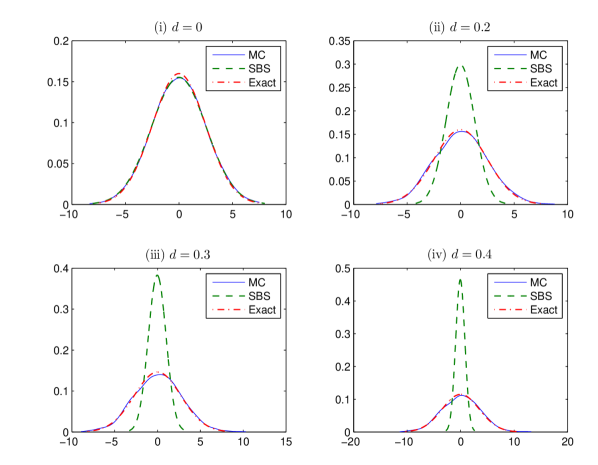
Figure 1: Densities of the re-normalized sample mean under ARFIMA$(1,d,0)$ with $T=500$, $\phi=0.6$, and $d=0,0.2,0.3,0.4$: Monte Carlo (MC); averaged (raw) sieve bootstrap (SBS) and exact ($N(0,\overline{\omega}^{2}$)), where $\overline{\omega}^{2}=T^{1-2d}Var[\bar{y}_{T}]$, with $Var[\bar{y}_{T}]$ as given in (5.1).

When $d=0$ we can see that all three distributions are very nearly identical. When $d>0$, however, it is clear that the variance of $\bar{y}_{T}$ is substantially underestimated by the bootstrap procedure. This result is further confirmed by inspection of Table 1, which reports the ratio of the average SBS estimate of the standard deviation of $\bar{y}_{T}$ to the exact standard deviation given by the square root of (5.1), for $T=100$ and $500,$ and for $\phi=0.3$ and $0.6.$ The underestimation for $d>0$ is very marked for both values of $\phi$ and both sample sizes with, indeed, the degree of underestimation increasing with $\phi$ and there being no uniform tendency for improvement as the sample size increases.

Table 1 Standard deviation of $\bar{y}_{T}$: averaged SBS estimate as a percentage of $\sqrt{Var[\bar{y}_{T}]}$, with $Var[\bar{y}_{T}]$ as defined in (5.1).

			$d$
			0.0	0.2	0.3	0.4
$\phi$	$T$
0.3	100		95.6%	57.2%	42.6%	28%
	500		99.2%	48.6%	35.1%	22.8%
0.6	100		93.3%	60.2%	46%	31%
	500		99.1%	51.5%	36.8%	23.8%

The reason for the underestimation stems from the fact that the raw sieve bootstrap variance is

$$Var^{\ast}[\bar{y}_{T}^{\ast}]=\frac{1}{T}\sum_{k=1-T}^{T-1}(1-\frac{|k|}{T})\bar{\gamma}_{h}(k),$$

where $\bar{\gamma}_{h}(k)=\widehat{\gamma}(k)$, $k=0,1,\ldots,h$, and $\sum_{j=0}^{h}\bar{\phi}_{h}(j)\bar{\gamma}_{h}(k-j)=0$, $k=h+1,\ldots$, with $\widehat{\gamma}(k)=\frac{1}{T-k}{\textstyle\sum\nolimits_{t=1}^{T-k}}(y(t)-\bar{y}_{T})(y(t+k)-\bar{y}_{T})$; and Hosking (1996) shows that the $\widehat{\gamma}(k)$ can have substantial negative bias relative to the corresponding true values even for moderate to large samples, particularly when $d$ is large.

This phenomenon is illustrated in Figure 2, which depicts the theoretical autocovariance function and the value of $\widehat{\gamma}(k)$ for $k=0,\ldots,100$ obtained from samples of size $T=1000$, computed from two fractional noise (ARFIMA$(0,d,0)$) processes with $d=0.3$ and $d=0.4$, and averaged across the $R$ replications. Hosking (1996, Theorem 3) provides the following formula for the asymptotic bias of the autocovariances

$$E[\widehat{\gamma}(k)-\gamma(k)]\sim-\omega^{2}T^{2d-1}\,,$$ (5.6)

(with $\omega^{2}$ as defined in 5.2), which depends on $d$ but is independent of $k$. This feature is reflected in the simulated sample bias, computed as the difference between the mean of the simulated sample autocovariances at each lag $k$ and the corresponding true $\gamma(k)$. For $T=1000$ this estimated bias is in close accord with the asymptotic approximation in (5.6), as can be seen in Figure 2.

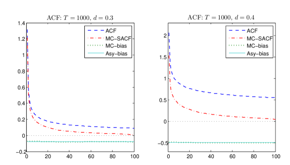
Figure 2: Theoretical autocovariance function (ACF); Monte-Carlo estimate of the expected sample autocovariance function (MC-SACF); Monte-Carlo estimate of the bias in the SACF (MC-Bias); and the asymptotic bias as per (5.6) (Asy-Bias), under fractional noise with $d=0.3,0.4$ and $T=1000$.

It is of interest then to ascertain whether the feasible PFSBS algorithm, in implicitly producing more accurate estimates of the $\gamma(k)$ in the process of yielding bootstrap draws of $\bar{y}_{T}$, (via the application of the sieve to a shorter memory process) yields an estimated sampling distribution for the mean with a variance that is closer to the theoretical value. As noted in Section 4, the PFSBS algorithm is based on a pre-filtering value of $d$ that is deemed to be “optimal” in the matching experimental design in Poskitt et al. (2012).

Figure 3 graphs the Monte Carlo distribution of $T^{1/2-d}(\bar{y}_{T}-\mu)$, the PFSBS distribution of $T^{1/2-d}(\bar{y}_{T}^{\ast}-\bar{y}_{T})$, and the $\mathbb{N}(0,\overline{\omega}^{2})$ distribution, for $T=500$, $\phi=0.6$, and $d=0,0.2,0.3,0.4$.

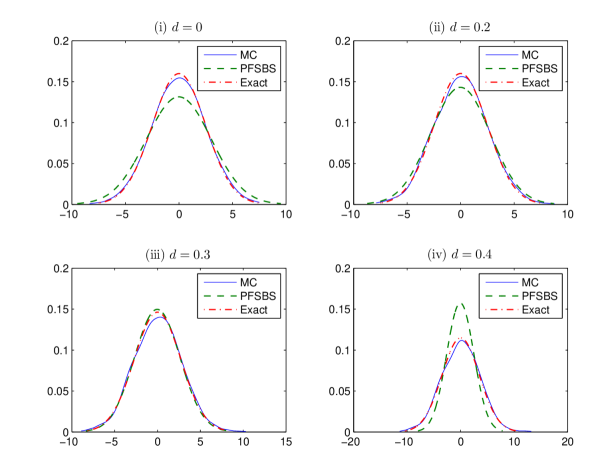
Figure 3: Densities of the re-normalized sample mean under ARFIMA$(1,d,0)$ with $T=500$, $\phi=0.6$, and $d=0,0.2,0.3,0.4$: Monte Carlo (MC); averaged pre-filtered sieve bootstrap (PFSBS) and exact ($N(0,\overline{\omega}^{2}$)), where $\overline{\omega}^{2}=T^{1-2d}Var[\bar{y}_{T}]$, with $Var[\bar{y}_{T}]$ as given in (5.1).

We see that, despite a tendency to over-estimate $Var(\bar{y}_{T})$ for $d=0$ and under-estimate for large $d$ ($d=0.4$), the PFSBS results are far superior to those associated with the raw SBS, and reasonably close overall to the true sampling distribution. The averaged PFSBS estimate of $\sqrt{Var\left(\bar{y}_{T}\right)}$ as a percentage of the true $\sqrt{Var\left(\bar{y}_{T}\right)}$ is presented in Panel A of Table 2, for the two values of $\phi$, $\phi=0.3$ and $0.6,$ and for $T=100$ and $500.$ The reasonable accuracy observed visually in Figure 3 for $\phi=0.6,$ for the larger sample size in particular, is broadly replicated for $\phi=0.3$, $T=500$, augering well for the automated use of the pre-filtering method in practice.

Table 2 Standard deviation of $\bar{y}_{T}$: averaged PFSBS and FPSBS estimates as a percentage of $\sqrt{Var[\bar{y}_{T}]}$, with $Var[\bar{y}_{T}]$ as defined in (5.1).

Panel A: PFSBS
		$d$
		$0.0$	$0.2$	$0.3$	$0.4$
$\phi$	$T$
0.3	100	141.2%	125.3%	109.8%	84.3%
	500	116.6%	106.9%	93.4%	69.9%
0.6	100	158.7%	142.9%	127.0%	100.4%
	500	117.1%	107.5%	94.0%	70.1%
Panel B: FPFBS
		$d$
		$0.0$	$0.2$	$0.3$	$0.4$
$\phi$	$T$
0.3	100	349.0%	191.1%	127.8%	74.3%
	500	573.4%	274.9%	171.6%	88.6%
0.6	100	316.0%	169.5%	115.7%	69.7%
	500	582.9%	268.6%	162.5%	84.7%

As a final point here, it is of interest to ascertain the performance of the PFSBS technique in which we simply assign a value to $d$ with which to pre-filter, rather than selecting a particular estimator for this role. A fairly obvious choice is to set the pre-filtering value ($d^{f}$ say) at $0.5;$ as the true $d$ (in the experimental setting) is never greater than this it follows that imposing $d^{f}=0.5$ results in a filtered series for which the effective fractional integration is always negative, and the filtered process of intermediate memory as a consequence. The estimates of the sieve parameters will therefore converge at the best possible rate $O\left(hT^{-1}\log T\right)$ as per Theorem 3, although $d^{f}$ will obviously not satisfy the convergence properties outlined in the discussion following Theorem 11. We refer to this approach below as the “fixed pre-filtered bootstrap” (FPFBS).

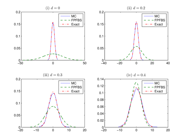
Figure 4: Densities of the re-normalized sample mean under ARFIMA$(1,d,0)$ with $T=500$, $\phi=0.6$, and $d=0,0.2,0.3,0.4$: Monte Carlo (MC); averaged fixed pre-filtered sieve bootstrap (FPFBS) and exact ($N(0,\overline{\omega}^{2}$)), where $\overline{\omega}^{2}=T^{1-2d}Var[\bar{y}_{T}]$, with $Var[\bar{y}_{T}]$ as given in (5.1).

As we see from Figure 4, the FPFBS, unsurprisingly, works reasonably well when $d$ is large; i.e., for $d=0.4.$ For the smaller values for $d$, on the other hand, it works very poorly, resulting in an averaged bootstrap distribution for $\bar{y}_{T}$ that is a very inaccurate match for the true distribution. In particular, as seen in panels (i) – (iii) of the Figure, and in Panel B of Table 2, the dispersion of the FPFBS-based distribution is much larger than that of the exact distribution, with the discrepancy increasing with the distance $\left|d-d^{f}\right|.$ In short, it appears that fixing the pre-filter is not useful as a default setting, at least as regards estimating the distribution of $\bar{y}_{T}$.

5.3 Simulation results: sample autocorrelation

We begin by plotting various estimates of the true finite sampling distribution of $\widehat{\rho}_{0}(k),$ for $k=1,3,6$ and $9,$ where the subscript $0$ is used to emphasize that a mean of zero (for $y_{t}$) is both assumed and imposed in the calculation of the statistic (see (5.4)). We consider this particular version of the autocorrelation coefficient(s) in this initial exercise so as to enable the LRZ expansion (derived for this version) to be used as a comparator. The expansion is valid for $d<0.1$ only (see Appendix); hence we conduct the comparison for a value of $d$ in this range: $d=0.08.$ Results for $\phi=0.3$ and $\phi=0.6$ are presented in Figures 5 and 6 respectively, with $T=500$ in both cases.

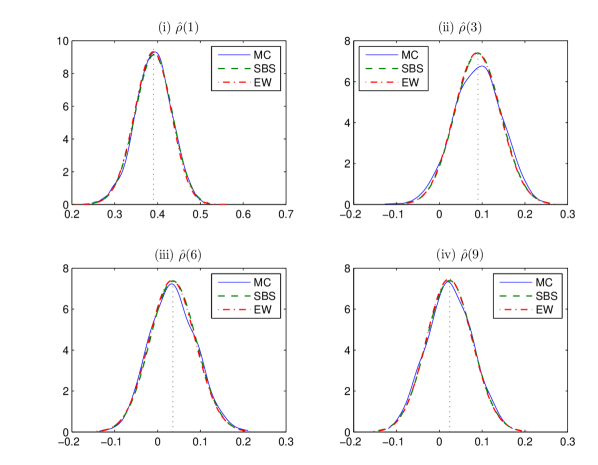
Figure 5: Densities of the zero-mean sample autocorrelation coefficient $\hat{\rho}_{0}(k)$, $k=1,3,6,9$: under ARFIMA$(1,d,0)$ with $T=500$, $d=0.08$, $\phi=0.3$: Monte Carlo (MC); averaged (raw) sieve bootstrap (SBS); Edgeworth approximation (EW). The vertical dotted line indicates the position of the true value of $\rho(k)$, $k=1,3,6,9.$

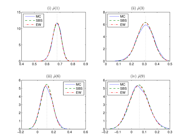
Figure 6: Densities of the zero-mean sample autocorrelation coefficient $\hat{\rho}_{0}(k)$, $k=1,3,6,9$: under ARFIMA$(1,d,0)$ with $T=500$, $d=0.08$, $\phi=0.6$: Monte Carlo (MC); averaged (raw) sieve bootstrap (SBS); Edgeworth approximation (EW). The vertical dotted line indicates the position of the true value of $\rho(k)$, $k=1,3,6,9.$

As is evident from inspection of the two graphs, the (raw) SBS estimate of the distribution of $\widehat{\rho}_{0}(k)$ is visually indistinguishable from the Edgeworth distribution, with both being very similar to the Monte Carlo based estimate. As such, we conclude that when a finite sample comparator is available (i.e. under the conditions required for that comparator to be valid) the sieve bootstrap method is remarkably accurate. This gives one confidence in the ability of the bootstrap to provide an accurate result in the usual case in which such a comparator is unavailable.

In Figures 7–10 we proceed to document the performance of the two bootstrap methods, SBS and PFSBS, in regions of the parameter space in which the Edgeworth expansion is not valid, and the only comparator is the Monte Carlo-based estimate of the exact sampling distribution. We also include plots of the average FPFBS distributions calculated using, as in the previous section, $d^{f}=0.5.$ The distribution for the sample autocorrelation coefficient in (5.3) is now the one documented, for $k=1,$ $3,$ $6$ and $9$, and the two scenarios considered are that in which asymptotic normality holds ($d\leq 0.25),$ and that in which it does not $(d>0.25)$, with the modified Rosenblatt distribution being the relevant limiting form in the latter case. Specifically, in Figures 7 and 8, $d=0.2$ and $\phi=0.3$ and $\phi=0.6$ respectively, whilst in Figures 9 and 10, $d=0.4$ and $\phi=0.3$ and $\phi=0.6$ respectively. In order to supplement these graphical results, the measures of fit (as described in Section 5.1) are recorded in both panels of Table 3, in relative terms. That is, in Panel A, each fit measure for PFSBS is presented as a ratio to the corresponding fit measure for the raw sieve method (SBS); hence, a value less than one indicates that the pre-filtering yields a distribution that is a better fit to the Monte Carlo-based distribution. The corresponding results for FPFBS are presented in Panel B. Results recorded in all four figures and both panels of the table are for $T=500.$

A visual inspection of the graphs in Figures 7 and 8 suggests that when the long memory parameter is small $(d=0.2)$, and for both values of $\phi$, the two bootstrap methods, SBS and PFSBS, provide reasonable accuracy.

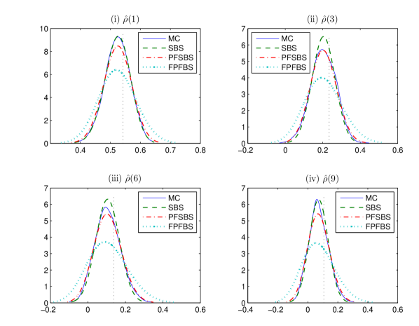
Figure 7: Densities of the sample autocorrelation coefficient $\hat{\rho}(k)$, $k=1,3,6,9$: under ARFIMA$(1,d,0)$ with $T=500$, $d=0.2$, $\phi=0.3$: Monte Carlo (MC); averaged (raw) sieve bootstrap (SBS); averaged pre-filtered sieve bootstrap (PFSBS); averaged fixed pre-filtered sieve bootstrap (FPFBS). The vertical dotted line indicates the position of the true value of $\rho(k)$, $k=1,3,6,9.$

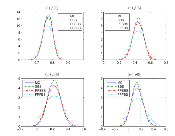
Figure 8: Densities of the sample autocorrelation coefficient $\hat{\rho}(k)$, $k=1,3,6,9$: under ARFIMA$(1,d,0)$ with $T=500$, $d=0.2$, $\phi=0.6$: Monte Carlo (MC); averaged (raw) sieve bootstrap (SBS); averaged pre-filtered sieve bootstrap (PFSBS); averaged fixed pre-filtered sieve bootstrap (FPFBS). The vertical dotted line indicates the position of the true value of $\rho(k)$, $k=1,3,6,9.$

There is no clear cut superiority of one method over the other, with the raw sieve method being superior to the PFSBS method for $k=1$ and $9$, and the opposite result obtaining for $k=3$ and $6.$ These visual results on relative performance are confirmed (overall) by the numerical results in Table 3, Panel A, with virtually all ratios (associated with all three measures of fit) being greater than one (indicating the superiority of the raw method) for $k=1$ and $9,$ and less than one for $k=3$ and $6.$

In contrast, for $d=0.4$, the performances of the two methods are more distinct, with all graphs reproduced in Figures 9 and 10 - allied with the numerical results reported in Panel A, Table 3 - confirming the marked superiority of the PFSBS method in this part of the parameter space. Taken together these two sets of results suggest that a conservative approach to estimating the sampling distribution of the autocorrelation coefficients in empirical settings is to undertake the pre-filtering; the increase in accuracy in the long memory region being worth the slight reduction that may occur (relative to the raw sieve) if the true value of $d$ is small.

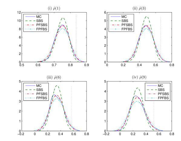
Figure 9: Densities of the sample autocorrelation coefficient $\hat{\rho}(k)$, $k=1,3,6,9$: under ARFIMA$(1,d,0)$ with $T=500$, $d=0.4$, $\phi=0.3$: Monte Carlo (MC); averaged (raw) sieve bootstrap (SBS); averaged pre-filtered sieve bootstrap (PFSBS); averaged fixed pre-filtered sieve bootstrap (FPFBS). The vertical dotted line indicates the position of the true value of $\rho(k)$, $k=1,3,6,9.$

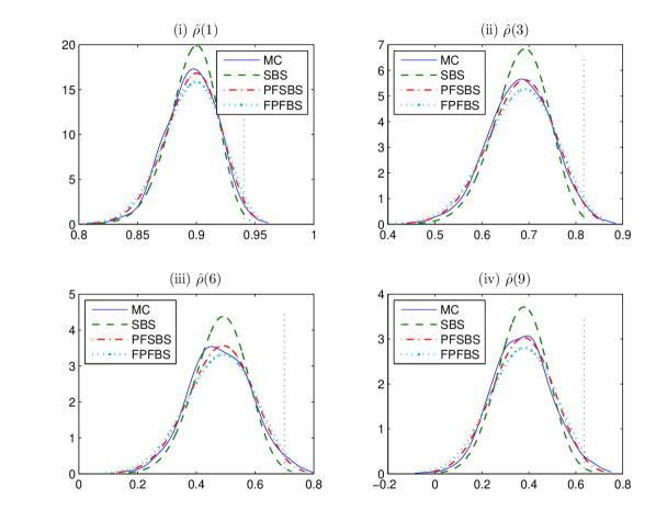
Figure 10: Densities of the sample autocorrelation coefficient $\hat{\rho}(k)$, $k=1,3,6,9$: under ARFIMA$(1,d,0)$ with $T=500$, $d=0.4$, $\phi=0.6$: Monte Carlo (MC); averaged (raw) sieve bootstrap (SBS); averaged pre-filtered sieve bootstrap (PFSBS); averaged fixed pre-filtered sieve bootstrap (FPFBS). The vertical dotted line indicates the position of the true value of $\rho(k)$, $k=1,3,6,9.$

Table 3 Goodness of fit measures for $\hat{\rho}(k)$, $k=1,3,6,9$:
measures for PFSBS and FPFBS relative to those for SBS.
All results are for sample size $T=500$.

		Panel A: PFSBS
		$d=0.2$					$d=0.4$
		Lag length $k$					Lag length $k$
		$1$	$3$	$6$	$9$		$1$	$3$	$6$	$9$
	$\phi$
RMSE	0.3	4.566	0.384	0.616	1.276		0.235	0.173	0.358	0.374
	0.6	1.467	0.520	0.682	1.343		0.322	0.233	0.392	0.387
KLD	0.3	12.26	0.733	1.087	1.579		0.302	0.095	0.141	0.163
	0.6	6.357	1.304	0.858	1.310		0.500	0.130	0.195	0.231
GINI	0.3	9.006	0.339	0.605	1.128		0.264	0.128	0.234	0.333
	0.6	2.679	0.418	0.611	1.211		0.370	0.220	0.290	0.349
		Panel B: FPFBS
		$d=0.2$					$d=0.4$
		Lag length $k$					Lag length $k$
		$1$	$3$	$6$	$9$		$1$	$3$	$6$	$9$
	$\phi$
RMSE	0.3	16.52	2.472	3.597	4.486		0.597	0.409	0.567	0.797
	0.6	4.385	2.416	2.699	4.257		0.597	0.436	0.530	0.662
KLD	0.3	102.99	10.32	18.79	18.18		0.971	0.380	0.426	0.507
	0.6	34.030	13.110	9.644	11.15		1.129	0.447	0.425	0.491
GINI	0.3	36.173	3.239	4.117	5.522		0.743	0.471	0.548	0.794
	0.6	9.979	2.946	3.220	4.829		0.759	0.502	0.519	0.655

Turning, finally, to the FPFBS, from inspection of Figures 7-10 and the results recorded in Panel B of Table 3, we see that while it virtually always outperforms the raw SBS for the larger value of $d$ ($d=0.4$), it does very poorly for $d=0.2$. In the latter case we observe a “divergence” (as measured by our three goodness of fit measures) from the Monte Carlo distribution we are attempting to replicate that is several times larger than that of SBS; more than 100 times larger in one case. Most importantly, if we compare the FPFBS directly to the PFSBS (by making the appropriate simple calculations using the numbers recorded in the two panels of Table 3) we see that the FPSBS never outperforms the PFSBS, with the goodness of fit measures for the former ranging from (approximately) twice to seventeen times those of the latter. This poor performance (overall) of the FPFBS mimics that documented for the sample mean.

6 Summary and Conclusion

This paper has derived new results regarding the convergence rates of sieve-based bootstrap techniques, in the context of fractionally integrated processes. Both the raw sieve technique, based on an autoregressive approximation of the long memory process, and a pre-filtered version of the sieve method, are investigated, for a broad class of statistics that includes the sample mean and sample second-order moments. Pre-filtering via an appropriate estimator is shown to yield a convergence rate that is equivalent to that associated with intermediate and short memory processes, which is, in turn, arbitrarily close to that associated with independent data.

Using numerical simulation, the distinct (and only rarely noted) problem of underestimating the sampling variance of the sample mean in the long memory case is shown to be avoided, in large measure, by use of a pre-filtering method based, in turn, on a (bias-adjusted) semi-parametric estimator of the long memory parameter. In particular, for moderate values of $d$ the pre-filtered sieve produces very accurate estimates of the (known) exact distribution of the sample mean, and achieves reasonable accuracy elsewhere in the parameter space. Replacing the data-based pre-filter with a fixed value may produce a slight improvement, but only when the latter is close to the true parameter; otherwise the fixed pre-filtering performs very badly in terms of reproducing the exact distribution.

The (data-based) pre-filtering technique is also shown to produce very accurate estimates of the true sampling distribution of selected autocorrelation coefficients (as measured by Monte Carlo simulation). Whilst there is no clear cut superiority of the pre-filtered over the raw sieve method when the fractional integration parameter is small, as the fractional integration parameter increases the performance of the two methods becomes more distinct, and the pre-filtering method performs notably better, reflecting the properties established in the theoretical development. As is the case with the sample mean, while fixed pre-filtering can outperform the raw method when the assigned pre-filtering value is close to the true parameter, it does very poorly otherwise, and in any case never outperforms data-based pre-filtering in terms of reproducing the (Monte Carlo) sampling distributions of the sample autocorrelations. Finally, for the narrow region of the parameter space in which an Edgeworth approximation of the distribution of the sample autocorrelations is valid, the sieve bootstrap reproduces this analytical result with great accuracy.

With due acknowledgement made of the limited nature of the current experimental exercise, we conclude that the overall increase in accuracy obtained when using the data-based pre-filtered sieve bootstrap in parts of the parameter space associated with moderate to strong long-range dependence is worth the slight reduction that might occur (relative to the raw sieve) otherwise; and that a reasonable approach to estimating unknown sampling distributions in empirical settings is to employ the data-based pre-filtered sieve as the default method.

Appendix A Edgeworth expansion for the sample autocorrelation function

To support the reproducibility of the results reported in this paper, we provide a brief outline of the details of the Edgeworth expansion used as a comparator of our bootstrap-based methodology. All further details of this expansion can be found in Lieberman et al. (2001) (LRZ hereafter).

Suppose we possess a statistic $s_{T}$ such that $\zeta_{T}=\sqrt{T}(s_{T}-E[s_{T}])\overset{\mathcal{D}}{\rightarrow}\mathbb{N}(0,\nu^{2})$. The conventional (second-order) Edgeworth expansion for the CDF of $\zeta_{T}$ is of the form

$$F_{\zeta_{T}}(c) =\Pr\left\{\zeta_{T}<c=\nu u\right\}$$ (A.1)

$$=G\left(u\right)-\left\{\frac{\eta_{3}}{6\sqrt{T}}H_{2}\left(u\right)+\frac{1}{T}\left(\frac{\eta_{4}}{24}H_{3}\left(u\right)+\frac{\eta_{3}^{2}}{72}H_{5}\left(u\right)\right)\right\}g\left(u\right)+O\left(T^{-3/2}\right)$$

where $\eta_{r}=\left.\kappa_{r}\right/\nu^{r}$ denotes the $r^{th}$ standardised cumulant of $\zeta_{T},$ and

$$H_{2}\left(u\right) =u^{2}-1$$

$$H_{3}\left(u\right) =u^{3}-3u$$

$$H_{5}\left(u\right) =u^{5}-10u^{3}+15u$$

are the required Hermite polynomials (Hall, 1992). Accordingly, direct application of (A.1) to the statistic

$$W_{T}(k)=\sqrt{T}\left(\hat{\rho}(k)-\rho(k)\right)$$ (A.2)

requires a means of computing the required cumulants of $W$. In theory these might be computed via Magnus (1986, Theorem 6), or possibly Smith (1989); in practice these expressions quickly become unmanageable as the order of the required moments increases.

LRZ instead begin with

$$Z_{T}(k)=\sqrt{n}\left(\hat{\gamma}(k)-\gamma(k)\right),$$ (A.3)

where

$$\widehat{\gamma}(k) =\frac{1}{T}\sum_{t=1}^{T-k}x(t)x(T+k)=T^{-1}x^{\prime}A_{T,k}x\,,$$

$$\left[A_{T,k}\right]_{i,j} =\xi_{k}\left(i-j\right)=\left\{\begin{array}[c]{cl}\frac{1}{2}&\text{for}\quad\left|i-j\right|=k\\ 0&\text{otherwise}\end{array}\right.,$$

and $A_{T,0}=I_{T}$. Assuming that $x=(x(1),\ldots,x(T))^{\prime}$ is distributed $\mathbb{N}\left(0,\Sigma\right)$, LRZ then proceed to produce an expansion for $W_{T}(k)$ indirectly, via $Z_{T}(k)$, as follows.

For brevity write $Z_{T}(k)$ and $W_{T}(k)$ as $Z_{k}$ and $W_{k}$ respectively, and use $\rho(k)=\gamma(k)/\gamma(0)$ and $\hat{\gamma}(k)=\gamma(k)+T^{-1/2}Z_{k}$ to now rewrite $W_{k}$ as

$$W_{k} =\sqrt{T}\left(\frac{\hat{\gamma}(k)}{\hat{\gamma}(0)}-\frac{\gamma(k)}{\gamma(0)}\right)$$

$$=\sqrt{T}\left(\frac{\hat{\gamma}(k)\gamma(0)-\gamma(k)\hat{\gamma}(0)}{\hat{\gamma}(0)\gamma(0)}\right)$$

$$=\frac{\gamma(0)Z_{k}-\gamma(k)Z_{0}}{\gamma(0)\hat{\gamma}(0)}$$

$$=\frac{Z_{k}-\rho(k)Z_{0}}{\hat{\gamma}(0)}.$$

Then for a single $W_{k}:$

$$F_{W_{k}}(c) =\Pr\left(W_{k}<c\right)$$

$$=\Pr\left(Z_{k}-\rho(k)Z_{0}<c\hat{\gamma}(0)\right)\quad\text{since }\hat{\gamma}(0)>0$$

$$=\Pr\left(Z_{k}-\rho(k)Z_{0}<c\gamma(0)+cT^{-1/2}Z_{0}\right)$$

$$=\Pr\left(Z_{k}-\left(\rho(k)+cT^{-1/2}\right)Z_{0}<c\gamma(0)\right),$$

where, from (A.3),

$$Z_{k}-\left(\rho(k)+cT^{-1/2}\right)Z_{0} =\sqrt{T}\left(\hat{\gamma}(k)-\left(\rho(k)+cT^{-1/2}\right)\hat{\gamma}(0)\right)$$

$$-\left[\sqrt{T}\left(\gamma(k)-\left(\rho(k)+cT^{-1/2}\right)\gamma(0)\right)\right]$$

$$=\sqrt{T}\left(\hat{\gamma}(k)-\left(\rho(k)+cT^{-1/2}\right)\hat{\gamma}(0)\right)+c\gamma(0)$$

$$=\sqrt{T}\left(n^{-1}x^{\prime}A_{T,k}x-\left(\rho(k)+cT^{-1/2}\right)T^{-1}x^{\prime}x\right)+c\gamma(0)$$

$$=T^{-1/2}x^{\prime}B_{T,k}x+c\gamma(0)$$

and $B_{T,k}=A_{T,k}-\left(\rho(k)+cT^{-1/2}\right)I_{T}.$ So, defining $x^{\prime}B_{T,k}x=Q_{T,k}^{{\dagger}},$ we have

$$F_{W_{k}}(c)=\Pr\left(W_{k}<c\right)\equiv\Pr\left\{Q_{T,k}^{{\dagger}}<0\right\}.$$

Standard results on quadratic forms in normal variates when $x\sim\mathbb{N}(0,\Sigma)$ gives $\psi_{T}(\tau)=E[i\tau Q_{T,k}^{{\dagger}}]=\prod_{t=1}^{T}(1-2i\tau\lambda_{t})^{-\frac{1}{2}}$ on application of Aitken’s integral, where $\lambda_{t}$, $t=1,\ldots,T$ are the eigenvalues of $B_{T,k}\mathbf{\Sigma}$. The characteristic function is integrable for all $T>2$ and the cumulant generating function $-\frac{1}{2}\sum_{t=1}^{T}\log(1-2i\tau\lambda_{t})$ yields the $r^{th}$ cumulant of $Q_{T,k}^{{\dagger}}$ as

$$\kappa_{r}^{\ast}=2^{r-1}\left(r-1\right)!\mathrm{tr}\left[\left(B_{T,k}\mathbf{\Sigma}\right)^{r}\right]\,.$$

Evaluating the mean and variance now makes $Q_{T,k}^{{\dagger}}$ (or more correctly its $z$-score) a convenient candidate for an Edgeworth expansion.

From the preceding,

$$F_{W_{k}}(c)\equiv\Pr\left\{Q_{T,k}^{{\dagger}}<0\right\}=\Pr\left\{\frac{Q_{T,k}^{{\dagger}}-\mu^{{\dagger}}}{\sigma^{{\dagger}}}<u=-\frac{\mu^{{\dagger}}}{\sigma^{{\dagger}}}\right\},$$

where $\mu^{{\dagger}}=\kappa_{1}^{{\dagger}}$ and $\sigma^{{\dagger}}=\sqrt{\kappa_{2}^{{\dagger}}}$. Hence the second-order Edgeworth expansion (if it exists) for the CDF of $Q_{T,k}^{{\dagger}}$ (and hence $W_{k})$ will be of the form

$$\widetilde{F}_{W_{k}}(c)=G\left(u\right)-\left\{\frac{\eta_{3}^{{\dagger}}}{6}H_{2}\left(u\right)+\frac{\eta_{4}^{{\dagger}}}{24}H_{3}\left(u\right)+\frac{(\eta_{3}^{{\dagger}})^{2}}{72}H_{5}\left(u\right)\right\}g\left(u\right),$$

with error $O\left(T^{-3/2}\right),$ where $\eta_{r}^{{\dagger}}=\kappa_{r}^{{\dagger}}/(\sqrt{\kappa_{2}^{{\dagger}}})^{r}$, $r=1,2,3,4$, and $u=-\eta_{1}^{{\dagger}}$. Note that the descending powers of $\sqrt{T}$ that would ordinarily appear in the expansion (cf. (A.1)) are here subsumed into the standardised cumulants; that is, we are implicitly assuming that $\eta_{r}^{{\dagger}}=O\left(T^{1-r/2}\right)$ or, equivalently, that $\kappa_{r}^{{\dagger}}$ is $O\left(T\right)$, at least up to $r=4$.

That the cumulants of $Q_{T,k}^{{\dagger}}$ are of the appropriate order, at least for restricted values of the fractional parameter $d,$ follows from LRZ Theorem 1. In particular, the cumulants of $Q_{T,k}^{{\dagger}}$ of order no greater than $r$ will be $O\left(T\right)$ only if $r(2d)<1$, implying that $\kappa_{r}^{{\dagger}}$, $r=1,2,3,4$, are $O\left(T\right)$ if $d<0.125$ but not otherwise. However, if $r$ now denotes the order of the highest cumulant in the expansion, then LRZ also show that we require $(r+1)(2d)<1$ and $r$ even to attain an expansion error of $o\left(T^{1-r/2}\right)$; while if $r$ is odd the error is of the same order as the last term, namely $O\left(T^{1-r/2}\right)$. Hence the second-order ($r=4$) expansion is valid only for $d<0.1$, and there is no valid expansion (in the sense that the error is of smaller order than the last included term) for $d\geq 0.1$.

References

- Adenstedt (1974) Adenstedt, R. K. (1974). On large–sample estimation for the mean of a stationary sequence. The Annals of Statistics 2 1095–1107.
- Andrews et al. (2006) Andrews, D. W., Lieberman, O. and Marmer, V. (2006). Higher-order improvements of the parametric bootstrap for long-memory Gaussian processes. Journal of Econometrics 133 673–702.
- Andrews and Lieberman (2005) Andrews, D. W. K. and Lieberman, O. (2005). Valid edgeworth expansions for the Whittle maximum likelihood estimator for stationary long-memory gaussian time series. Econometric Theory 21 710–734.
- Andrews and Sun (2004) Andrews, D. W. K. and Sun, Y. (2004). Adaptive local polynomial Whittle estimation of long-range dependence. Econometrica 72 569–614.
- Apostol (1960) Apostol, T. M. (1960). Mathematical Analysis. Addison-Wesley, Reading.
- Beran (1994) Beran, J. (1994). Statistics for long-memory processes, vol. 61 of Monographs on Statistics and Applied Probability. Chapman and Hall, New York.
- Beran (1995) Beran, J. (1995). Maximum likelihood estimation of the differencing parameter for invertible short and long memory autoregressive integrated moving average models. Journal of the Royal Statistical Society B 57 654–672.
- Bickel and Freedman (1981) Bickel, P. J. and Freedman, D. A. (1981). Some asymptotic theory for the bootstrap. Annals of Statistics 9 1196–1217.
- Brockwell and Davis (1991) Brockwell, P. J. and Davis, R. A. (1991). Time Series: Theory and Methods. Springer Series in Statistics. Springer-Verlag, New York, 2nd ed.
- Bühlmann (1997) Bühlmann, P. (1997). Sieve bootstrap for time series. Bernoulli 3 123–148.
- Choi and Hall (2000) Choi, E. and Hall, P. G. (2000). Bootstrap confidence regions from autoregressions of arbitrary order. Journal of the Royal Statistical Society B 62 461–477.
- Dahlhaus (1989) Dahlhaus, R. (1989). Efficient parameter estimation for self-similar processes. Annals of Statistics 17 1749–1766.
- Doornik and Ooms (2001) Doornik, J. A. and Ooms, M. (2001). Computational aspects of maximum likelihood estimation of autoregressive fractionally integrated moving average models. Computational Statistics & Data Analysis 42 333–348. Also a 2001 Nuffield discussion paper.
- Durbin (1980) Durbin, J. (1980). Approximations for densities of sufficient estimators. Biometrika 67 311–333.
- Fox and Taqqu (1986) Fox, R. and Taqqu, M. S. (1986). Large sample properties of parameter estimates for strongly dependent stationary gaussian time series. Annals of Statistics 14 517–532.
- Geweke and Porter-Hudak (1983) Geweke, J. and Porter-Hudak, S. (1983). The estimation and application of long-memory time series models. Journal of Time Series Analysis 4 221–238.
- Giraitis and Robinson (2003) Giraitis, L. and Robinson, P. M. (2003). Edgeworth expansions for semiparametric Whittle estimation of long memory. Annals of Statistics 31 1325–1375.
- Granger and Joyeux (1980) Granger, C. W. J. and Joyeux, R. (1980). An introduction to long-memory time series models and fractional differencing. Journal of Time Series Analysis 1 15–29.
- Hall (1992) Hall, P. (1992). The bootstrap and Edgeworth expansion. Springer series in Statistics. Springer-Verlag, New York.
- Hesterberg (1997) Hesterberg, T. (1997). Matched-block bootstrap for long memory processes. Research Report 66, MathSoft, Inc, Seattle, WA.
- Hosking (1980) Hosking, J. R. M. (1980). Fractional differencing. Biometrika 68 165–176.
- Hosking (1996) Hosking, J. R. M. (1996). Asymptotic distributions of the sample mean, autocovariances, and autocorrelations of long memory time series. Journal of Econometrics 73 261–284.
- Inoue and Kasahara (2006) Inoue, A. and Kasahara, Y. (2006). Explicit representation of finite predictor coefficients and its applications. Annals of Statistics 34 973–993.
- Kreiss et al. (2011) Kreiss, J. P., Paparoditis, E. and Politis, D. N. (2011). On the range of validity of the autoregressive sieve bootstrap. Annals of Statistics 39 2103–2130.
- Künsch (1989) Künsch, H. R. (1989). The jacknife and the bootstrap for general stationary observations. Annals of Statistics 17 1217–1241.
- Lieberman and Phillips (2004) Lieberman, O. and Phillips, P. C. B. (2004). Expansions for the distribution of the maximum likelihood estimator of the fractional difference parameter. Econometric Theory 20 464–484.
- Lieberman et al. (2001) Lieberman, O., Rousseau, J. and Zucker, D. M. (2001). Valid Edgeworth expansion for the sample autocorrelation function under long range dependence. Econometric Theory 17 257–275.
- Lieberman et al. (2003) Lieberman, O., Rousseau, J. and Zucker, D. M. (2003). Valid asymptotic expansions for the maximum likelihood estimator of the parameter of a stationary, gaussian, strongly dependent process. The Annals of Statistics 31 586–612.
- Magnus (1986) Magnus, J. R. (1986). The exact moments of a ratio of quadratic forms in normal variables. Annals of Economics and Statistics / Annales d’ conomie et de Statistique pp. 95–109.
- Nielsen and Frederiksen (2005) Nielsen, M. . and Frederiksen, P. H. (2005). Finite sample comparison of parametric, semiparametric, and wavelet estimators of fractional integration. Econometric Reviews 24 405–443.
- Politis (2003) Politis, D. N. (2003). The impact of bootstrap methods on time series analysis. Statistical Science 219–230.
- Poskitt (1994) Poskitt, D. S. (1994). A note on autoregressive modelling. Econometric Theory 10 884–899.
- Poskitt (2007) Poskitt, D. S. (2007). Autoregressive approximation in nonstandard situations: The fractionally integrated and non-invertible cases. Annals of Institute of Statistical Mathematics 59 697–725.
- Poskitt (2008) Poskitt, D. S. (2008). Properties of the sieve bootstrap for fractionally integrated and non-invertible processes. Journal of Time Series Analysis 29 224–250.
- Poskitt et al. (2012) Poskitt, D. S., Martin, G. M. and Grose, S. G. (2012). Bias reduction of long memory parameter estimators via the pre-filtered sieve bootstrap. Econometrics & Business Statistics Working Paper WP 08/12, Monash University.
- Robinson (1995a) Robinson, P. M. (1995a). Gaussian semiparametric estimation of long range dependence. Annals of Statistics 23 1630–1661.
- Robinson (1995b) Robinson, P. M. (1995b). Log periodogram regression of time series with long memory. Annals of Statistics 23 1048–1072.
- Shibata (1980) Shibata, R. (1980). Asymptotically efficient selection of the order of the model for estimating parameters of a linear process. Annals of Statistics 8 147–164.
- Smith (1989) Smith, M. D. (1989). On the expectation of a ratio of quadratic forms in normal variables. Journal of Multivariate Analysis 31 244–257.
- Sowell (1992) Sowell, F. (1992). Maximum likelihood estmation of stationary univariate fractionally integrated time series models. Journal of Econometrics 53 165–188.
- Taniguchi (1984) Taniguchi, M. (1984). Validity of Edgeworth expansions for statistics of time series. Journal of Time Series Analysis 5 37–51.