Dynamic connectivity algorithms for Monte Carlo simulations of the random-cluster model

Abstract

We review Sweeny’s algorithm for Monte Carlo simulations of the random cluster model. Straightforward implementations suffer from the problem of computational critical slowing down, where the computational effort per edge operation scales with a power of the system size. By using a tailored dynamic connectivity algorithm we are able to perform all operations with a poly-logarithmic computational effort. This approach is shown to be efficient in keeping online connectivity information and is of use for a number of applications also beyond cluster-update simulations, for instance in monitoring droplet shape transitions. As the handling of the relevant data structures is non-trivial, we provide a Python module with a full implementation for future reference.

1 Introduction

The cluster-update algorithm introduced for simulations of the Potts model by Swendsen and Wang in 1987 [1] has been a spectacular success, reducing the effect of critical slowing down by many orders of magnitude for the system sizes typically considered in computer simulation studies. A number of generalizations, including an algorithm for continuous-spin systems and the single-cluster variant [2] as well as more general frameworks for cluster updates [3, 4], have been suggested following the initial work of Ref. [1]. The single bond update introduced by Sweeny [5] several years before Swendsen’s and Wang’s work is considerably less well known. This is mostly due to difficulties in its efficient implementation in a computer code, which is significantly more involved than for the Swendsen-Wang algorithm. In deciding about switching the state of a given bond from inactive to active or vice versa, one must know the consequences of the move for the connectivity properties of the ensemble of clusters, i.e., whether two previously disjoint clusters will become connected or an existing cluster is broken up by the move or, instead, the number of clusters will stay unaffected. If implemented naively, these connectivity queries require a number of steps which is asymptotically close to proportional to the number of spins, such that the resulting computational critical slowing down outweighs the benefit of the reduced autocorrelation times of the updating scheme. Even though it was recently shown that the decorrelation effect of the single-bond approach is asymptotically stronger than that of the Swendsen-Wang approach [6, 7], this strength can only be played once the computational critical slowing down is brought under control. Here, we use a poly-logarithmic dynamic connectivity algorithm as recently suggested in the computer science literature [8, 9, 10] to perform bond insertion and removal operations as well as connectivity checks in run-times only logarithmically growing with system size, thus removing the problem of algorithmic slowing down. As the mechanism as well as the underlying data structures for these methods are not widely known in the statistical physics community, we here use the opportunity to present a detailed description of the approach. For the convenience of the reader, we also provide a Python class implementing these codes, which can be used for simulations of the random-cluster model or rather easily adapted to different problems where dynamic connectivity information is required.

2 The random-cluster model and Sweeny’s algorithm

We consider the random-cluster model (RCM) [11] which is a generalization of the bond percolation problem introducing a correlation between sites and bonds. It is linked to the $q$-state Potts model through the Fortuin-Kasteleyn transformation [12, 13, 14], generalizing the Potts model to arbitrary real $q>0$. Special cases include regular, uncorrelated bond percolation ($q=1$) as well as the Ising model ($q=2$). To define the RCM, consider a graph $\mathcal{G}\equiv(V,E)$ with vertex set $V$, ($|V|\equiv N$), and edge set $E$, ($|E|\equiv M$). We associate an occupation variable $\omega(e)\in\{0,1\}$ with every edge $e\in E$. We say that $e$ is active if $\omega(e)=1$ and inactive otherwise. The state space $\Omega$ of the RCM corresponds to the space of all (spanning) sub-graphs,

$$\Omega\equiv\{\mathcal{A}=(V,A)|A\subseteq E\}=\{0,1\}^{M}.$$ (1)

A configuration is thus represented as $\vec{\omega}\equiv[\omega(e_{1}),\omega(e_{2}),...,\omega(e_{M})]\in\Omega$ and corresponds uniquely to a sub-graph $\mathcal{A(\vec{\omega})}\equiv(V,A(\vec{\omega}))\subseteq\mathcal{G}$ with

$$A(\vec{\omega})=\{e\in E|\omega(e)=1\}\subseteq E.$$ (2)

The probability associated with a configuration $\vec{\omega}\in\Omega$ is given by the RCM probability density function (PDF)

$$\mu(p,q,\vec{\omega}) \equiv \frac{1}{Z(p,q)}\left[\prod_{e\in E}p^{\omega(e)}(1-p)^{1-\omega(e)}\right]q^{k(\vec{\omega})},$$ (3)

$$Z(p,q) \equiv \sum_{\vec{\omega}\in\Omega}\left[\prod_{e\in E}p^{\omega(e)}(1-p)^{1-\omega(e)}\right]q^{k(\vec{\omega})},$$ (4)

where $k(\vec{\omega})$ is the number of connected components (clusters) and $Z(p,q)$ denotes the RCM partition function. More generally, as a function of the parameters $p\in[0,1]$, the density of active edges, and $q\in(0,\infty)$, the cluster number weight, these expressions define a family of PDFs. It is worthwhile to mention a number of limiting cases. For $q\rightarrow 1$ Eq. (3) factorizes and corresponds to independent bond percolation with $Z(p)\rightarrow 1$. In the limit of $q\rightarrow 0$ with fixed ratio $w=v/q$, on the other hand, it corresponds to bond percolation with local probability $w/(1+w)$ and the condition of cycle-free graphs. Taking $w\rightarrow\infty$ or in the limit of $q\rightarrow 0$ and $v/q^{\sigma}$ constant for $0<\sigma<1$ we obtain the ensemble of uniform spanning trees for connected $G$. Naturally, in the latter two limits every edge in a configuration is a bridge.

Sweeny’s algorithm [5] is a local bond updating algorithm directly implementing the configurational weight (3). We first consider its formulation for the limiting case $q\to 1$ of independent bond percolation. For an update move, randomly choose an edge $e\in E$ with uniform probability and propose a flip of its state from inactive to active or vice versa. Move acceptance can be implemented with any scheme satisfying detailed balance, for instance the Metropolis acceptance ratio $\min{(v^{\Delta w},1)}$ where $v\equiv p/(1-p)$ and $\Delta\omega=\pm 1$ for insertions and deletions of edges, respectively. This dynamical process is described by the following master equation:

$$\mathbb{P}(\vec{\omega},t+1)=(1-r(\vec{\omega}))\mathbb{P}(\vec{\omega},t)+\sum_{\vec{\omega}^{\prime}\neq\vec{\omega}}W(\vec{\omega}^{\prime}\rightarrow\vec{\omega})\mathbb{P}(\vec{\omega^{\prime}},t),$$ (5)

where $r(\vec{\omega})=\sum_{\vec{\omega}^{\prime}\neq\vec{\omega}}W(\vec{\omega}\rightarrow\vec{\omega^{\prime}})$ ensures proper normalization of $\mathbb{P}(\vec{\omega},t+1)$, given the normalization of $\mathbb{P}(\vec{\omega},t)$ . The Metropolis transition rates are then given by

$$W(\vec{\omega}\rightarrow\vec{\omega}^{\prime}) \equiv \frac{1}{M}\sum_{m=1}^{M}W_{m}(\vec{\omega}\rightarrow\vec{\omega}^{\prime}),$$ (6)

$$W_{m}(\vec{\omega}\rightarrow\vec{\omega}^{\prime}) \equiv \min{(1,v^{\Delta w})}\prod_{l\neq m}\left[\delta_{\omega_{l},\omega_{l}^{\prime}}\right].$$ (7)

Eq. (6) expresses the uniform random selection of an edge and the corresponding edge dependent transition rate $W_{m}$ is defined in Eq. (7). The product of Kronecker deltas ensures the single-bond update mechanism, i.e., that only one edge per step is changed. From here, generalization to arbitrary $q\in(0,\infty)$ is straightforward, leading to a modified transition rate

$$W_{m}(\vec{\omega} \rightarrow \vec{\omega}^{\prime})\equiv\ \min(1,q^{\Delta k}v^{\Delta\omega})\prod_{l\neq m}\left[\delta_{\omega_{l},\omega_{l}^{\prime}}\right].$$ (8)

We note that this Metropolis update is more efficient than a heat-bath variant for any value of $q$ apart from $q=1$, where both rules coincide. Clearly, for $q\neq 1$, to compute the acceptance probability $W_{m}$ of a given trial move one must find $\Delta k$, the change in connected components (clusters) induced by the move. This quantity, equivalent to the question of whether the edge $e$ is a bridge, is highly non-local. Determining it involves deciding whether there exists at least one alternative path of active edges connecting the incident vertices $x$ and $y$ that does not cross $e=(x,y)$.

3 The connectivity problem

The dynamic connectivity problem is the task of performing efficient connectivity queries to decide whether two vertices $x$ and $y$ are in the same ($x\leftrightarrow y$) or different ($x\nleftrightarrow y$) connected components for a dynamically evolving graph, i.e., mixing connectivity queries with edge deletions and insertions. For a static graph, such information can be acquired in asymptotically constant time after a single decomposition, for instance using the Hoshen-Kopelman algorithm [15]. Under a sequence of edge insertions (but no deletions), it is still possible to perform all operations, insertions and connectivity queries, in practically constant time using a so-called union-and-find (UF) data structure combined with path-compression and tree-balance heuristics [16]. This fact has been used to implement a very efficient algorithm for the (uncorrelated) percolation problem [17]. An implementation of Sweeny’s algorithm, however, requires insertions as well as deletions to ensure balance. Hence, we need to be able to remove edges without the need to rebuild the data structure from scratch.

Table 1: Asymptotic run-time scaling at criticality of the elementary operations of insertion or deletion of internal or external edges, respectively, using sequential breadth-first search (SBFS), interleaved BFS (IBFS), union-and-find (UF) or the fully dynamic connectivity algorithm (DC) as a function of the linear system size $L$.

operation	SBFS	IBFS	UF	DC
internal insertion	$L^{d_{F}-x_{2}}$	$L^{d_{F}-x_{2}}$	const.	$\log^{2}L$
external insertion	$L^{\gamma/\nu}$	$L^{d_{F}-x_{2}}$	const.	$\log^{2}L$
internal deletion	$L^{d_{F}-x_{2}}$	$L^{d_{F}-x_{2}}$	$L^{d_{F}-x_{2}}$	$\log^{2}L$
external deletion	$L^{\gamma/\nu}$	$L^{d_{F}-x_{2}}$	$L^{\gamma/\nu}$	$\log^{2}L$
dominant	$L^{\gamma/\nu}$	$L^{d_{F}-x_{2}}$	$L^{\gamma/\nu}$	$\log^{2}L$

This goal can be reached using a number of different techniques. Building on the favorable behavior of the UF method under edge insertions and connectivity queries, the data structure can be updated under the removal of an external edge (bridge) by performing breadth-first searches (BFSs) through the components connected to the two ends $x$ and $y$ of the edge $e=(x,y)$. Alternatively, one might try to do without any underlying data structure, answering each connectivity query through a separate graph search in breadth-first manner. In both cases, the process can be considerably sped up by replacing the BFSs by interleaved traversals alternating between vertices on the two sides of the initial edge and terminating the process as soon as one of the two searches comes to an end [18, 19, 7]. As, at criticality of the model, the sizes of the two cluster fragments in case of a bridge bond turn out to be very uneven on average, this seemingly innocent trick leads to dramatic run-time improvements [7]. The asymptotic run-time behavior of insertion and deletion steps for internal and external edges and the algorithms based on BFS or UF data structures is summarized in Table 1 for the case of simulations on the square lattice of edge length $L$. We expect the same bounds with the corresponding exponents to hold for general critical hypercubic lattices. Here, $\gamma/\nu$ denotes the finite-size scaling exponent of the susceptibility and $d_{F}-x_{2}$ is a geometric exponent related to the two-arm crossing behavior of clusters [19]. We note that $d_{F}-x_{2}<\gamma/\nu$ for $0<q\leq 4$ in two dimensions. Asymptotically, it is the most expensive operation which dominates the run-time of the algorithm and, as a consequence, it turns out that (for the square lattice) a simple BFS with interleaving is more efficient than the approach based on union-and-find, cf. Table 1.

In any case, the implementations discussed so far feature a computational effort for a sweep of bond updates that scales faster than linearly with the system size, thus entailing some computational critical slowing down. It is found in Ref. [7] that for most choices of $q$, this effect appears to asymptotically destroy any advantage of a faster decorrelation of configurations by the Sweeny algorithm as compared to the Swendsen-Wang method. An alternative technique based on more complicated data structures allows to perform any mix of edge insertions, deletions and connectivity queries in poly-logarithmic run-time per operation [8, 9, 10]. Poly-logarithmic here denotes polynomials of powers of the logarithm of the independent variable, e.g., system size $L$, of the form

$$f(L)=\sum_{k=0}^{K}\alpha_{k}\log^{k}L.$$ (9)

Here the base of the logarithm is not important and changes only the coefficients. In the following all logarithms are with respect to base $2$. Given the observation of generally faster decorrelation of configurations by the Sweeny algorithm in the sense of smaller dynamical critical exponents [6, 7], the use of such (genuinely) dynamic connectivity algorithms (DC) allows for an asymptotically more efficient simulation of the critical random-cluster model [7]. In the following, we discuss the basic ideas and some details of the algorithm employed here.

3.1 Trees, Forests and Euler tours

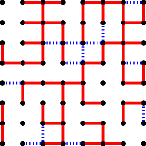
(a) Level $0$.

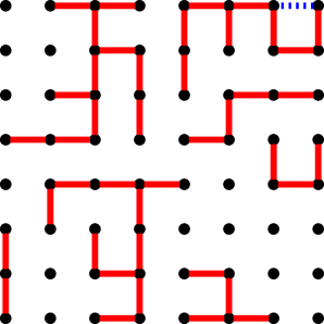
(b) Level $1$.

Figure 1: A sub-graph $\mathcal{A}$ of a $8\times 8$ square lattice. The solid (red) lines correspond to edges in one spanning forest $\mathcal{F}(\mathcal{A})$ and the dashed (blue) lines are additional edges not in the current spanning forest. Note that the graph has periodic boundary conditions and hence there are edges wrapping around the lattice horizontally and vertically. For the sake of clarity these are not shown.

The DC algorithm is based on the observation that for a given sub-graph $\mathcal{A}$ it is possible to construct a spanning forest $\mathcal{F}(\mathcal{A})$ which is defined by the following properties:

• $x\leftrightarrow y$ in $\mathcal{F}(\mathcal{A})$ if and only if $x\leftrightarrow y$ in $\mathcal{A}$

• there exists exactly one path for every pair $x$, $y$ with $x\leftrightarrow y$

In other words a spanning forest of a graph associates a spanning tree to every component, an example is given in Fig. 1a (solid lines only). One advantage of $\mathcal{F}(\mathcal{A})$ is that it has fewer edges than ${\cal A}$, but represents the same connectivity information. For the sub-graph ${\cal A}$, the distinction of tree edges $e\in\mathcal{F}(\mathcal{A})$ and non-tree edges $e\in\mathcal{A}\backslash\mathcal{F}(\mathcal{A})$ allows for a cheap determination of $\Delta k$. For the case of deleting an edge in $e\notin\mathcal{F}(A)$ we know that there is an alternative path connecting the adjacent vertices, namely the path in $\mathcal{F}(\mathcal{A})$, so this edge was part of a cycle and we conclude $\Delta k=0$. If we insert an edge whose adjacent vertices are already connected in $\mathcal{F}(\mathcal{A})$ then we come to the same conclusion.

If, on the other hand, we want to insert a tree edge, i.e., an edge with adjacent vertices $x$, $y$ not yet connected, we observe that because $x$ and $y$ belong to separate spanning trees before the insertion of $e$, the new spanning subgraph obtained by linking $x$ and $y$ via $e$ is still a spanning tree. Hence the only modification on the spanning forest for the insertion of a tree edge is the amalgamation of two trees. This can be done in $\mathcal{O}(\log L)$ steps by using the following idea of Ref. [20] which also supports the deletion of bridges. For a given component $\mathcal{C}$ in $\mathcal{A}$ we transform the corresponding tree $\mathcal{T}(\mathcal{C})$ in $\mathcal{F}(\mathcal{A})$ into a directed circuit by replacing every edge $(x,y)$ by two directed edges (arcs) $[x,y]$ and $[y,x]$ and every vertex by a loop $[x,x]$. Figure 2 illustrates how to translate edge insertions or deletions into/from the spanning forest to modifications on the directed circuits. Deleting an edge from a tree splits it into two trees. The directed circuit therefore splits into two circuits corresponding to the two trees. When inserting a tree edge, i.e., merging two trees, we join the circuit by the two arcs, corresponding to $e$, at the vertices incident to $e$.

By storing the directed circuits for every component in so called Euler tour sequences (ETS), [8], all necessary manipulations on the directed circuits can be done in $\mathcal{O}(\log L)$ operations if we store each ETS in a separate balanced search tree such as, for instance, a red-black, AVL, or B tree [21]. Alternatively one can use self-adjusting binary search trees, so called splay trees [22]. In this case the bound is amortized, i.e., averaged over the complete sequence of operations. Due to a somewhat simpler implementation and the fact that a Monte Carlo simulation usually consists of millions of operations in random order naturally leading to amortization, we concentrated on the splay-tree approach. Based on the ETS representation we can translate connectivity queries into checking the underlying search tree roots for equivalence. An in-depth discussion of the exact manipulations on the representing ETS is beyond the scope of this article and we refer the interested reader to the literature [8]. Here we restrict ourselves to considering the deletion of a bridge as an example. The initial graph is the one illustrated in the left panel of Fig. 2. One corresponding ETS sequence of the linearized directed cycle in the right panel of Fig. 2 is the following:

$$\mathcal{E}=[1,1]\rightarrow[1,2]\rightarrow[2,2]\rightarrow[2,4]\rightarrow[4,4]\rightarrow[4,3]\rightarrow[3,3]\rightarrow[3,4]\rightarrow[4,2]\rightarrow[2,1].$$ (10)

Suppose now that we delete edge $(2,4)$ from the tree (cf. the dashed line in Fig. 2). This will result in a split of the component $\mathcal{C}\equiv\{1,2,3,4\}$ into two parts $\mathcal{C}_{1}\equiv\{1,2\}$ and $\mathcal{C}_{2}\equiv\{3,4\}$. In this case the deletion of edge $(2,4)$ translates into a cut of the original sequence $\mathcal{E}$ at the two arcs $[2,4]$ and $[4,2]$. The sequence $\mathcal{E}_{2}$ of arcs between these two edges corresponds to $\mathcal{C}_{2}$ and the concatenation of the remaining sequences without the two arcs corresponding to $(2,4)$ results in $\mathcal{E}_{1}$ representing $\mathcal{C}_{1}$:

$$\mathcal{E}_{1} = [1,1]\rightarrow[1,2]\rightarrow[2,2]\rightarrow[2,1],$$ (11)

$$\mathcal{E}_{2} = [4,4]\rightarrow[4,3]\rightarrow[3,3]\rightarrow[3,4].$$ (12)

In summary, we see that by mapping every component in $\mathcal{A}$ to a tree in $\mathcal{F}(\mathcal{A})$ and every such tree to a directed circuit which we store in an ETS we are able to perform edge insertions/deletions into/from $\mathcal{F}(A)$ as well as connectivity queries with an amortised $\mathcal{O}(\log L)$ computational effort.

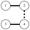
      $\mapsto$      

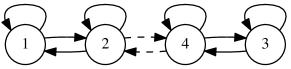
Figure 2: Mapping of a component to a directed circuit with loops. The dashed line is an edge to be deleted. The dashed arrows will be removed to update the directed circuit.

3.2 Edge hierarchy

The remaining operation not implemented efficiently by the provisions discussed so far is the deletion of edges from $\mathcal{F}(\mathcal{A})$ which are not bridges, i.e., for which a replacement edge exists outside of the spanning forest. The DC algorithm first executes the tree splitting as in the case of a bridge deletion. Additionally, however, it checks for a reconnecting edge in the set of non-tree edges. If such an edge is found, it concludes $\Delta k=0$ and merges the two temporary trees as indicated above by using the located non-tree edge, which hence now becomes a tree edge. If, on the other hand, no re-connecting edge is found, no additional work is necessary as the initially considered edge is a bridge. To speed up the search for replacement edges, we limit it to the smaller of the two parts $\mathcal{C}_{1}$ and $\mathcal{C}_{2}$ as all potential replacement edges must be incident to both components. To allow for efficient searches for non-tree edges incident to a given component using the ETS representation, the search-tree data structures are augmented such that the loop arc for every vertex stores an adjacency list of non-tree edges (vertices) incident to it. Further, every node in the underlying search tree representing the ETS carries a flag indicating if any non-tree edge is available in the sub-tree [which is a sub-tree of the search tree and not of $\mathcal{F}(\mathcal{A})$]. This allows for a search of replacement edges using the Euler tour and ensures that any non-tree edge can be accessed in $\mathcal{O}(\log L)$ time.

It turns out that exploiting this observation is, in general, beneficial but not sufficient to ensure the amortized time complexity bound indicated for the DC algorithm in general. Suppose that the graph consists of a giant homogeneous component with $M=\alpha N$ and $0<\alpha\leq 1$ and the edge deletion results, temporarily setting aside the question of possible replacement edges, in two trees with $\alpha_{1}N$ and $(\alpha-\alpha_{1})N$ incident edges, respectively, where $0<\alpha_{1}\leq\alpha/2$. Then the computational effort caused by scanning all possible non-tree edges is clearly $\mathcal{O}(N)$. In amortizing onto the insertions performed to build up this component, every such non-tree edge carries a weight of $\mathcal{O}(\log L)$. If this case occurs sufficiently frequently, it will be impossible to bound the amortized cost per operation. This problem is ultimately solved in the DC algorithm by the introduction of an edge hierarchy. The intuitive idea is to use the expense of a replacement edge search following a deletion to reduce the cost of future operations on this edge. This is done in such a way as to separate dense from sparse clusters and more central edges from those in the periphery of clusters. By amortizing the cost of non-tree edge scans and level increases over edge insertions it follows that one can reduce the run-time for graph manipulations to an amortized $\mathcal{O}(\log^{2}L)$ and $\mathcal{O}(\log L)$ for connectivity queries [9]. Each time an incident non-tree edge is checked and found unsuitable for reconnecting the previously split cluster we promote it to be in a higher level. If we do this many times for a dense component we will be able to find incident non-tree edges very quickly in a higher level. These ideas are achieved in the DC algorithm by associating a level function to each $e\in E$,

$$0\leq\ell(e)\leq\ell_{\max}\equiv\lfloor\log N\rfloor.$$ (13)

Based on this level function, one then constructs sub-graphs $\mathcal{A}_{i}\subseteq\mathcal{A}$ with the property

$$\mathcal{A}_{i}\equiv\{e\in\mathcal{A}|l(e)\geq i\}.$$ (14)

This induces a hierarchy of sub-graphs:

$$\mathcal{A}_{\ell_{\max}}\subseteq\cdots\subseteq\mathcal{A}_{1}\subseteq\mathcal{A}_{0}\equiv\mathcal{A}.$$ (15)

As described above, for every sub-graph we construct a spanning forest $\mathcal{F}_{i}\equiv\mathcal{F}(\mathcal{A}_{i})$. Clearly the same hierarchy holds for the family of spanning forests. In other words the edges in level $i-1$ connect components/trees of level $i$. If an edge has to be inserted into $\mathcal{A}$, then it is associated to a level $l(e)=0$ and hence it is in $\mathcal{A}_{0}$. To achieve an efficient search for replacement edges, the algorithm adapts the level of edges after deletions of tree edges in a way which preserves the following two invariants [9]:

1. The maximal number of vertices in a component in level $i$ is $\lfloor N/2^{i}\rfloor$.

2. Any possible replacement edge for a previously deleted edge $e$ with level $l$ has level $\leq l$.

Trivially, both invariants are fulfilled when all edges have level 0. We now have to specify how exactly the idea of keeping important edges at low levels and unimportant ones at higher levels is implemented. To do this, suppose we deleted an edge from $\mathcal{F}_{i}$, i.e., at level $i$, and temporarily have $\mathcal{T}\rightarrow\mathcal{T}_{1}+\mathcal{T}_{2}$ where (say) $\mathcal{T}_{1}$ is the smaller of the two, i.e., it has less vertices. Because of invariant (i) it follows that we are allowed to move the tree $\mathcal{T}_{1}$ (which is now at most half the size of $\mathcal{T}$) to level $i+1$ by increasing the level of all tree edges of $\mathcal{T}_{1}$ by one. After that we start to search for a replacement edge in the set of non-tree edges stored in the ETS of $\mathcal{T}_{1}$ in level $i$ where it also remains because of the fact that $\mathcal{F}_{i+1}\subseteq\mathcal{F}_{i}$. For every scanned non-tree edge we have two options:

• It does not reconnect $\mathcal{T}_{1}$ and $\mathcal{T}_{2}$ and has therefore both ends incident to $\mathcal{T}_{1}$. In this case, we increase the level of this edge $i\rightarrow i+1$. This implements the idea of moving unimportant edges in “dense” components to higher levels.

• It does reconnect and hence we re-insert it at level $0$.

If we have not found a replacement edge at level $i$ we continue at level $i-1$. The search terminates after unsuccessfully completing the search at level $0$ or when a replacement edge was found. In the first case it follows $\mathcal{C}\rightarrow\mathcal{C}_{1}+\mathcal{C}_{2}$ whereas in the second case $\mathcal{C}$ remains unchanged.

Implementing this replacement-edge search following any tree-edge deletion introduces an upward flow of edges in the hierarchy of graphs and the level of an edge in the current graph never decreases. Focusing on a single edge, we see that it is sequentially moved into levels of smaller cluster size and hence the cost of future operations on this edge is reduced. Taking this into account it follows that the insertion of an edge has a cost of $\mathcal{O}(\log L)$ for inserting at level $0$ plus it also “carries” the cost of all possible $\mathcal{O}(\log L)$ level increases with cost of $\mathcal{O}(\log L)$ each resulting in $\mathcal{O}(\log^{2}L)$ amortized per insertion. Deletions on the other hand imply a split of cost $\mathcal{O}(\log L)$ in $\mathcal{O}(\log L)$ levels. In case of an existing replacement edge another contribution of $\mathcal{O}(\log L)$ caused by an insertion at level 0 is added. The contribution of moving tree edges to higher levels and searching for replacement edges (moving non-tree edges up) is already paid for by the sequence of previous insertions (amortization). The only missing contribution is the $\mathcal{O}(\log L)$ effort for obtaining the next replacement edge in an ETS. In total, deletions hence have an amortized computational cost of $\mathcal{O}(\log^{2}L)$.

3.3 Performance and optimizations

We tested the performance of the current DC implementation in the context of Sweeny’s algorithm in comparison to the simpler approaches based on breadth-first search and union-and-find strategies. While the algorithm discussed here allows all operations to be performed in poly-logarithmic time, due to the complicated data structures the constants are relatively large. Our results show consistency with the poly-logarithmic run-time bounds derived. It appears, however, that very large system sizes are required to clearly see the superior asymptotic performance of the DC algorithm as compared to the BFS and UF implementations. For details see the more elaborate discussion in Ref. [7]. As an example, Fig. 3 shows the average run-time per edge operation as a function of the system size for three different choices of parameters.

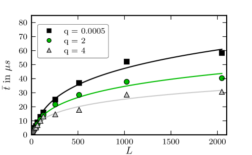
Figure 3: Average run-time for Sweeny’s algorithm for the RCM for different values of $q$ at the critical point $v_{c}=\sqrt{q}$ on the 2D square lattice with periodic boundary conditions.

Apart from run-time considerations, the implementation has a rather significant space complexity. Since we maintain $\mathcal{O}(\log L)$ overlapping forests over the $L^{2}$ vertices, the space complexity is $\mathcal{O}(L^{2}\log L)$. A heuristic suggested in Ref. [10] to decrease memory consumption is a truncation of higher edge levels as these are, for the inputs or graphs considered in our application, sparsely populated. We checked the impact on our implementation by comparing run-times and memory consumptions for a truncation $\ell_{\max}\rightarrow\ell_{\max}/2$. We did not see any significant change in the run-time. On the other hand we observed a reduction of almost a factor of two in the memory consumption. This conforms to our observation that during the course of a simulation almost no edges reached levels beyond $\approx 10$ for system sizes $L\lesssim 1024$ where the actual maximal level according to Eq. (13) is $\ell_{\max}=20$.

Likewise, a number of further optimizations or heuristics are conceivable to improve the typical run-time behavior. This includes a sampling of nearby edges when looking for a replacement edge before actually descending into the edge level hierarchy [10]. A number of such heuristics and experimental comparisons of fully and partially dynamics connectivity algorithms has been discussed in the recent literature, see Refs. [23, 24, 25]. A full exploration of these possibilities towards an optimal implementation of the DC class of algorithms for the purpose of the Sweeny update is beyond the scope of the current article and forms a promising direction for future extensions of the present work.

4 Sweeny Python class

We provide a Python class [26] encompassing four different implementations of Sweeny’s algorithm based on:

• sequential breadth-first searches (SBFS)

• interleaved breadth-first searches (IBFS)

• union-and-find with interleaved breadth-first searches (UF)

• poly-logarithmic dynamic connectivities as discussed here (DC)

The package is built on top of a C library and it is therefore possible to use the library in a stand-alone compiled binary. The necessary source code is also provided. For more details see the related project documentation [26]. The source code is published under the MIT license [27]. Here we give a basic usage example, which simulates the RCM with $q=2$ (the Ising model) at $v_{c}=\sqrt{2}$, using an equilibration time of $1000$ sweeps, a simulation length of $10000$ sweeps, and random number seed $1234567$ using the DC implementation:

Listing 1: Example usage of Sweeny class.

⬇

from sweeny import Sweeny

sy = Sweeny(q=2.,l=64,beta=np.log(1. + np.sqrt(2.)),coupl=1.,

cutoff=1000,tslength=10000,rngseed=1234567,impl=’dc’)

sy.simulate()

In order to extract an estimate, say, of the Binder cumulant $R=\langle\mathcal{S}_{4}\rangle/\langle\mathcal{S}_{2}^{2}\rangle$ we need to retrieve the time series for $\mathcal{S}_{4}$ and $\mathcal{S}_{2}$,

Listing 2: Retrieving time series.

⬇

sec_cs_moment= sy.ts_sec_cs_moment

four_cs_moment = sy.ts_four_cs_moment

sec_cs_moment *= sec_cs_moment

binder_cummulant = four_cs_moment.mean()/sec_cs_moment.mean()

Once an instance of the Sweeny class is created, it is easy to switch the algorithm and parameters as follows:

Listing 3: Switching algorithm and parameters.

⬇

sy.init_sim(q=1.3,l=64,beta=np.log(1.+np.sqrt(1.3.)),coupl=1.,

cutoff=5000,tslength=50000,rngseed=7434,impl=’ibfs’)

5 Conclusions

We have shown how to implement Sweeny’s algorithm using a poly-logarithmic dynamic connectivity method and we described the related algorithmic aspects in some detail. We hope that the availability of the source code and detailed explanations help to bridge the gap between the computer science literature on the topic of dynamic connectivity problems and the physics literature related to MC simulations of the RCM, specifically in the regime $q<1$.

The availability of an efficient dynamic connectivity algorithm opens up a number of opportunities for further research. This includes studies of the tricritical value $q_{c}(d)$ where the phase transition of the random-cluster model becomes discontinuous for dimensions $d>2$ [28, 18] as well as the nature of the ferromagnetic-paramagnetic transition for $q\rightarrow 0$ and $d>2$ [29].

E.M.E. would like to thank P. Mac Carron for carefully reading the manuscript.

References

References

- [1] Swendsen R H and Wang J S 1987 Phys. Rev. Lett. 58 86–88
- [2] Wolff U 1989 Phys. Rev. Lett. 62 361–364
- [3] Edwards R G and Sokal A D 1988 Phys. Rev. D 38 2009
- [4] Kandel D and Domany E 1991 Phys. Rev. B 43 8539–8548
- [5] Sweeny M 1983 Phys. Rev. B 27 4445
- [6] Deng Y, Garoni T M and Sokal A D 2007 Phys. Rev. Lett. 98 230602
- [7] Elçi E M and Weigel M 2013 Phys. Rev. E 88 033303
- [8] Henzinger M R and King V 1999 J. ACM 46 502–516
- [9] Holm J, de Lichtenberg K and Thorup M 2001 J. ACM 48 723–760
- [10] Iyer R, Karger D, Rahul H and Thorup M 2001 J. Exp. Algorithmics 6 4
- [11] Grimmett G 2006 The random-cluster model (Berlin: Springer)
- [12] Fortuin C M and Kasteleyn P W 1972 Physica 57 536–564
- [13] Fortuin C M 1972 Physica 58 393–418
- [14] Fortuin C M 1972 Physica 59 545–570
- [15] Hoshen J and Kopelman R 1976 Phys. Rev. B 14 3438–3445
- [16] Cormen T H, Leiserson C E, Rivest R L and Stein C 2009 Introduction to Algorithms 3rd ed (Cambridge, MA: MIT Press)
- [17] Newman M E J and Ziff R M 2001 Phys. Rev. E 64 016706
- [18] Weigel M 2010 Physics Procedia 3 1499–1513
- [19] Deng Y, Zhang W, Garoni T M, Sokal A D and Sportiello A 2010 Phys. Rev. E 81 020102
- [20] Tarjan R E 1997 Math. Program. 78
- [21] Knuth D E 1998 The Art of Computer Programming: Sorting and Searching v. 3: The Classic Work Newly Updated and Revised 2nd ed (Addison Wesley)
- [22] Sleator D D and Tarjan R E 1985 J. ACM 32 652–686
- [23] Zaroliagis C D 2002 Experimental Algorithmics (Lecture Notes in Computer Science vol 2547) ed Fleischer R, Moret B and Schmidt E (Springer Berlin Heidelberg) pp 229–278
- [24] Demetrescu C and Italiano G F 2006 ACM Trans. Algorithms 2 578–601
- [25] Demetrescu C, Eppstein D, Galil Z and Italiano G F 2010 ed Atallah M J and Blanton M (Chapman & Hall/CRC), chapter Dynamic graph algorithms, p 9
- [26] Elçi E M Sweeny Python module at Github, https://github.com/ernmeel/sweeny
- [27] MIT License, http://opensource.org/licenses/MIT
- [28] Hartmann A K 2005 Phys. Rev. Lett. 94 050601
- [29] Deng Y, Garoni T M and Sokal A D 2007 Phys. Rev. Lett. 98 030602