SmartLoc: Sensing Landmarks Silently for Smartphone Based Metropolitan Localization

Abstract

We present SmartLoc, a localization system to estimate the location and the traveling distance by leveraging the lower-power inertial sensors embedded in smartphones as a supplementary to GPS. To minimize the negative impact of sensor noises, SmartLoc exploits the intermittent strong GPS signals and uses the linear regression to build a prediction model which is based on the trace estimated from inertial sensors and the one computed from the GPS. Furthermore, we utilize landmarks (e.g., bridge, traffic lights) detected automatically and special driving patterns (e.g., turning, uphill, and downhill) from inertial sensory data to improve the localization accuracy when the GPS signal is weak. Our evaluations of SmartLoc in the city demonstrates its technique viability and significant localization accuracy improvement compared with GPS and other approaches: the error is approximately $20$m for $90\%$ of time while the known mean error of GPS is $42.22$m.

I Introduction

Localization have attracted significant attentions in the past few years, and numerous techniques have been proposed to achieve high accuracy localization. In outdoor scenarios, GPS and its variants are the most common technologies to provide accurate position for various applications [4]. However, problems caused by weak/none GPS signal in cities often lead to a pretty bad user experience. For instance, we conduct comprehensive experiments in downtown Chicago, IL USA, to evaluate the performance of GPS positioning. Based on the experiment results, we observe that the GPS signals are very weak and unstable in some roads due to highrises, or even blocked completely in some complicated road structures, such as tunnels and underground. In addition, the largest location error we collected is over $100$m on the ground, and nearly $400$m in the underground segments (see Fig. 1 for more details). Thus, improving the location accuracy is imperative when the GPS signal is weak.

In this work, we propose SmartLoc, a localization method which improves the localization accuracy in metropolises by leveraging embedded inertial sensors in smartphones to help improve the driving patterns according to various of road conditions. Exploiting the data collected from these inertial sensors has been used in the literature to address a number of challenging and interesting tasks, e.g., indoor localization [5, 28, 30, 14], road condition monitoring [16, 7], property tracking [9], and outdoor localization [9, 11, 20]. Note that some applications exploits accelerometer to measure walking speed and distance of pedestrian [3, 5, 23, 28] and exploit compass to estimate the direction so as to estimate the location. However, providing realtime localization of moving cars in metropolises is far more challenging as such activity does not have a cyclic pattern in sensory data.

To address these challenges, during the dead reckoning process for calculating the current position of a car, we propose a dynamic trajectory model to estimate the driving speed and velocity based on current road condition, so that the impact of inherent noise and accumulated error could be reduced to a large extent. We also design a calibration strategy based on road infrastructures (e.g., bridge, traffic lights, uphill, and downhill) and driving status (e.g., turns, stops), which are inferred from the sensory data. Our extensive evaluations indicate that leveraging inertial sensors could accurately identify the special road infrastructures using either fingerprint based approaches or pattern-matching technique.

We implement SmartLoc on Android, and evaluate the localization performance in both downtown Chicago and highway. Our extensive test results in the majority of blocks in Chicago indicate that SmartLoc improves the location accuracy significantly: 1) the mean localization error in each time slot is $11.65$m; 2) according to the proportion of ”good” road segments, the average localization error is less than $20$m such that the localization accuracy is increased from $\leq 50\%$ (by purely using GPS) to $\geq 90\%$ using SmartLoc in downtown areas. When testing SmartLoc on highway, the localization error is at most $12$m for $95\%$ of the time. In comparison the state-of-the-art localization scheme for moving vehicles, AutoWitness [9], only produces the error of distance estimation less than $10\%$ for most of the cases, which could be large when the estimated distance is long (e.g., $10\%$ of the 2 miles driving is $320$m). Our results also imply that SmartLoc can save the energy consumption by switching on/off the GPS periodically.

The main contributions of this work are summarized as follows:

1. We propose a self-learning driving model to reduce the speed and trajectory distance estimation error brought by both the inherent noise and dead-reckoning.

2. In a real scenario, when both the traffic condition and road infrastructures are complex and unpredictable, which hinder the trajectory estimation accurately, SmartLoc could adjust the self-learning driving model to calculate the best parameters to match the current driving condition.

3. Although self-calibration is a reliable approach to elevate the accuracy in localization, it is still difficult to calibrate the location in metropolises with weak GPS signal. SmartLoc also exploits the current coarse-grained estimation of location to confine the search space, so that a much more accurate localization could be achieved through matching the road infrastructures and driving status.

The rest of paper is organized as follows. We first review the state-of-art localization techniques in Section II. We show our measurement results and observations with respect to the GPS accuracy in Section III. We present the overview of SmartLoc in Section IV, following which novel calibration techniques of SmartLoc are presented one by one in Section V and Section VI. We report our detailed real-world experiment results in Section VII, and conclude the work in Section VIII.

II Related Works

Our work involves in a number of techniques, in this section, we mainly focus on the work related to wireless localization and dead-reckoning [13].

II-A Localization Techniques

GPS [15], being the most popular outdoor localization system, has been widely used to provide localization and navigation services to users such that numerous techniques have been proposed in the literature to improve the GPS localization accuracy, like A-GPS, D-GPS [21], WAAS [6], etc. Recently, WiFi signal [4, 1] and cellular signal [27, 2] have been used to find the locations as well. However, the median error for downtown environment based on cellular signal reaches $100$m at worst[2], and WiFi based solutions rely on nearby WiFi APs’ locations. Unfortunately, these GPS-based or WiFi-based solutions are inapplicable for navigation in metropolises because of many critical road infrastructures, such as under ground roads and multilayered roads where the GPS signal is often lost, and there are no WiFi access points at all. Some GSM-based localization methods, like [27, 16], are widely available. However, their accuracy is low (up to hundreds of meters) with the assumption that the exact positions of cellular towers should be known in priori.

Work PlaceLab [4], and ActiveCampus [8] make full use of WiFi and GSM signals for location at outdoor environment. The former creates a map by war-driving a region and maps both APs and cell tower’s signals to the wireless map. The latter is quite similar except it assumes the APs’ location is known in priori. Taking advantages of two aforementioned systems, CompAcc [5] uses dead-reckoning combined with AGPS to further calibrate localization results rather than utilizing preliminary war-driving. Unfortunately, all these systems need time-consuming calibration, and are not suitable for large scale area. Another work Skyhook [1] supply high accuracy location services with cost of hiring over $500$ drivers to create the WiFi/GSM map in certain region.

Several promising techniques such as crowdsourcing are introduced in localization recently, such as Zee [22], which also uses inertial sensors to track users’ movement.

II-B Dead-Reckoning

Recently, dead-reckoning strategies using internal sensors to estimate motion activities have attracted many research interests. Strapdown Inertial Navigation System (SINS) [26] and Pedometer System [12] use MEMS to estimate the moving speed and trace. The key issue is to deal with the noise of internal sensors and accumulated errors, which sometimes grow cubically [29]. Personal Dead-reckoning (PDR) system [19] uses “Zero Velocity Update” to calibrate the drift. The majority of the dead-reckoning studies focus on walking estimation, such as UnLoc [28], and CompAcc [5]. Their main idea is to use accelerometer sensors to estimate the number of walking steps, and then measure the walking distance. AutoWitness [9] is the system with an embedded wireless tag integrated with vibration, accelerometer, and gyroscope sensors. The tag is attached to a vehicle, and accelerometer and gyroscope sensors are used to track the moving trace.

II-C Road, Map and Traffic

Smartphones are used to analyze traffic patterns to provide better navigation system in vehicle. CTrack [24] and VTrack [25] are two systems which process error-prone positioning systems to estimate the trajectories. These two system match a sequence of observations on the transitions between locations, while the former adopt fingerprints and the latter mainly utilizes HMM. SmartRoad [10] detects and identifies traffic lights and stop signs through crowd-sensing strategies. Some research propose map matching algorithms based on Kalman Filter [18] or HMM [17]. However, such approaches cannot guarantee accuracy. IVMM [31] is then proposed to increase the accuracy.

III GPS Positioning in Downtown

III-A Measurement in Downtown Chicago

To study how bad the GPS location accuracy could be, we first conduct a comprehensive measurements of GPS accuracies within some area in Downtown Chicago, red rectangle shown in Figure 1(a). We drive through every road in the area while recording location information in a real-time manner. In order to remove the time dependent GPS location errors, we conduct independent measurements at three different times, and report the results by average. We find that in the test area, the largest location error reaches $400$m, and the distance of the longest road segment between two GPS locations with reasonable accuracies ($\leq 30m$) is about $1$km.

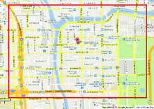
(a) Testing area in Chicago

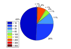
(b) Proportion of Error

Figure 1: GPS localization accuracy in Chicago.

III-B Original Location Results

Unfortunately, the location accuracy is not as high as expected according to our measurement results. For instance, the localization results have averagely $42.22$m errors and the largest error reaches $400$m, which is nearly the length of three blocks in downtown area. We further plot the localization accuracy information of downtown Chicago based on the measurement results in Figure 1(b). Clearly, only about half of the sampling points endure the error of less than $20$m, over one quarter of the locations have an error of about $50$m while the rest quarter has an error larger than $50$m.

We assume that the largest location error a user could accept inside a city should be less than $30$m, which is less than a quarter of one block. From now on, we consider the positions with GPS location error less than $30$m as the locations with good GPS signals, and the rest as the locations with bad GPS signals. Since longer segments of roads with bad GPS signals are prone to leading to wrong instruction for turning or stopping in a navigation system. We calculate the distance of road segments with bad GPS signal in the experiment area, and present the results in Figure 2. In Figure 2(a), we numbered each segment of road with bad GPS signal in X axis, and plot the length of all $182$ segments of road, which indicates that the longest length reaches almost one kilometer. Meanwhile, the Figure 2(b) illustrates the distribution of each segment of roads. We notice that the average length of these bad segments of road is approximately $200$m, and those with over $400$m locate in the center of downtown, which may confuse drivers most.

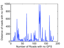
(a) Bad road segments.

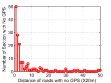
(b) Number of bad segments.

Figure 2: Road segments with poor GPS

IV System Overview

IV-A Main Idea

The objective of SmartLocis to use inertial sensors in smartphones to lively estimate the locations based on the trajectory and orientation through self-learnt dynamic model with high accuracy but low energy consumption. Remarkably, we not only address the inaccuracy caused by the complex infrastructures in downtown area, but also exploit them to improve the localization accuracy.

In trajectory measuring, traditional methods leveraging inertial sensors introduce large inherent errors, which leads to poor traveling distance and speed estimation. Besides the mechanism noise, such errors also come from the process of extracting and transforming linear acceleration in Earth Frame Coordinate and orientation estimation. Although Extended Kalman Filter could be adopted to reduce such coarse noise to some extent, trajectory calculating error still cannot be neglected. In the following stage, we propose a self-learning predictive regression model to estimate the moving distance based on the extracted acceleration, in which the accumulated errors are minimized in the following way. SmartLoc switches to the training process to train the predictive model when GPS signal is good. When GPS signals are unreliable, it uses the trained model to predict the moving trajectory of the vehicle. Due to the complex road conditions and unpredictable driving activities, the training process should be updated periodically in our model. In addition, SmartLoc also detects the landmarks by finding special patterns from sensory data when the car goes through bridges, tunnels, traffic lights or turning points, while calibrating the estimation accordingly.

IV-B Challenges

Many technical issues should be addressed here. The first issue is how to design an improved self-learning trajectory estimation model according to current driving conditions since naive methods using Newton’s Law accumulate the noises (e.g., when we double the integral on acceleration results in the displacement, the noises are doubly accumulated as well). The second issue is how to recognize the landmarks, which will be further used to improve the localization accuracy in our system. The last but not least challenge comes from the fact that even if some special landmarks are recognized, traffic conditions also affect the localization estimation accuracy, e.g., the unpredictable length of waiting queues in front of traffic lights. challenges in detail.

V Trajectory Calculation

V-A Background

Although accelerometer, gyroscope and magnetometer sensors could provide sensory data to reflect the motion conditions, the intrinsic noise could make the naive distance estimation based on Newton’s Law unavailable because the error will be accumulated.

Since drivers have been used to mount their smartphones on the windshield as navigators, and the orientation of the smartphone changes irregularly due to driving direction changing and vehicle vibration, we build an estimation model through gyroscope-based Extend Kalman Filter to decrease the orientation error, and extract linear acceleration in the coordinate of Earth.

V-B Self-learning Predictive Model

We observe from our preliminary experiments (Section III) that the majority of the road segments with bad GPS signals (error $\geq$ 30m) are usually shorter than $400$m, which takes about $20-30$ seconds to drive through in a normal condition. On the one hand, such distance is long enough to navigate drivers to wrong places, on the other hand it is short enough to endure the errors to some extent. Therefore, we propose the following predictive dynamic trajectory estimating model which adaptively calibrates itself using GPS signals and dead-reckoning.

Velocity Estimator: Because of the inherent noises and measurement errors, the traditional velocity estimation model is no longer reliable. In this case, we denote the velocity $V_{i}$ at the end of a timeslot $i$ as

$$V_{i}=V_{i-1}+\beta\cdot{a_{i}}\cdot{\Delta{t}}+\mu$$ (1)

where $\beta$ is the parameter to be learned and adjusted in real time, $a_{i}$ is the average measured acceleration during the timeslot $i$, and $\mu$ is the noise.

When GPS signals are strong, both $V_{i}$ and $V_{i-1}$ could be achieved from the GPS directly, and the mean linear acceleration $a_{i}$ is extracted from the accelerometer. Then we regress the model to find the best $\beta$, and calculate the noise $\mu$ hiding behind. When the localization through GPS is unreliable, we use the trained model proposed to predict the velocity $V_{i}$.

Distance Estimator: For general cases, the trajectory distance gathered from GPS indicates the distance with some error. Therefore, letting $G(\Delta{t}_{i})$ be the distance during a timeslot $i$ read from GPS, which could be presented as:

$$G(\Delta{t}_{i})={\lambda}_{1}\cdot{V_{i-1}}\cdot{\Delta{t}}+\frac{1}{2}\cdot{\widehat{a_{i}}}\cdot{\Delta{t}^{2}}+\eta$$

where $\widehat{a_{i}}$ is the actual acceleration in the time slot $i$. Here $\lambda_{1}$ is multiplied to reflect the error in the estimated speed $V_{i-1}$ for the time slot $i-1$. Since the known measured acceleration $a_{i}$ contains both inherent noise and measurement errors, by assuming that these error follows normal distribution, we define the measured acceleration as:

$$a_{i}=(1+\varepsilon)\widehat{a_{i}}+\delta,$$

where $\widehat{a_{i}}$ is considered as the true acceleration which cannot be obtained. Then, we use the following formula to estimate the distance $G(\Delta t_{i})$:

$$G(\Delta t_{i})={\lambda}_{1}\cdot{V_{i-1}}\cdot{\Delta{t}}+{\lambda}_{2}\frac{1}{2}\cdot{a_{i}}\cdot{\Delta{t}^{2}}+{\lambda}_{3}\cdot{\Delta{t}^{2}}+{\lambda}_{4}\cdot{\Delta{t}}+\eta$$ (2)

where $\lambda_{1},\cdots,\lambda_{4}$ are parameters to be learned by our regression model. When GPS signals are strong (GPS error is $\leq 20$m), based on the $V_{i-1}$, $a_{i}$ is computed using the sensory data and the distance from GPS, we train our model using Eq. (2), which is in turn used to predict the distance $G(\Delta{t}_{i})$ in the time slot $i$ when GPS signals are bad. From the predicted trajectory distance $G(\Delta t_{i})$, the location at the timeslot $i$ could be estimated based on the obtained location, distance and orientation.

However, since the location errors from GPS changes in both spacial and temporal dimensions, it is difficult to estimate the times and places at which GPS signals become weak. In addition, driving in downtown area face unpredictable traffic conditions and road infrastructures, which affects the parameters learnt from the previous model. Therefore, we propose a more flexible dynamic adjusting strategy to update the parameters to match the current driving status. In our strategy, we calculate the parameters in predictive dynamic trajectory estimating model only based on the latest driving data. We allocate a small buffer to save the latest driving informations. When the protocol is still in the learning process, the model will replace the oldest data with latest informations in order to update the model parameters. Based on our evaluation, the estimation accuracy in trajectory distance reduces to a large extent.

V-C Movement Detection

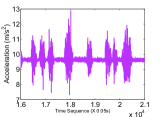
(a) Acceleration

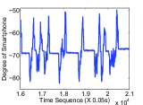
(b) BFC/EFC angle

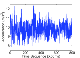
(c) Acceleration in Cruise

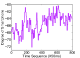
(d) BFC/EFC angle in Cruise

Figure 3: The Acceleration and Angle while driving in city or Cruise model.

Remembering that the speed estimator calculates speeds based on the accelerometer, and the speed contains noises accumulated from the integral. Therefore, even if the vehicle stops, the estimated speed is highly likely to be non-zero, which may lead to a huge error in the final prediction. Hence, determining whether the vehicle is moving or halting could further reduce the negative impact of the mechanical noises. In addition, movement detection is also the key to the process of landmark calibration, which adjusts the location when the vehicle stops in front of traffic lights or stop signs.

During our preliminary experiments, we find that the movement can be reflected precisely from both accelerometer and gyroscope sensors, as shown in Figure 3. The acceleration fluctuates frequently when the vehicle is in motion, even in cruise mode, and remains relatively stable when it stops (Figure 3(a) and 3(c)). The same situation occurs in the gyroscope (Figure 3(b) and 3(d)). Although the smartphone is usually mounted to the windshield, due to the inertia while driving, especially speeding up or brake, the gyroscope could still sense small rotation changes. For all the cases, we calculate the variance for readings from both sensors, and we find that the largest differences between two vehicles is stopping and moving. For the acceleration, the variance in motion is approximately $60$ times of that in still, with $0.01$ in stopping, $0.6$ and $0.4$ for regular driving and cruise mode. The differences of variance for gyroscope sensors are similar instead. SmartLoc continuously collect the sensory data from both accelerometer and gyroscope, if the vibration lies below the threshold, we consider the vehicle is stopped. In our experiment, we find that SmartLoc can differentiate moving and stopping activities precisely.

VI Calibration by Landmarks

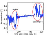
(a) Traffic lights

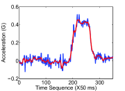
(b) Centripetal force

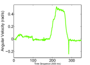
(c) Angular velocity

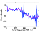
(d) Magnetometer

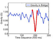
(e) Bridge

Figure 4: Pattern of the sensor data collected in different road infrastructures when driving: (a) car stopping and crossing a traffic light; (b), (c), and (d) car turning $90^{o}$; and (e) car crossing a bridge.

As we have mentioned before, the road infrastructures, including tunnels, bridges, crossroads and traffic lights, cause large noises in the GPS data, which results in a large drift in the distance estimation if it is not treated rigorously. In this work, we exploit the precise location of these infrastructures available in Google Map to calibrate the localization without any extra cost.

Traffic Light: When the vehicle stops due to the traffic lights and drives through crossroads, unique patterns appear in the readings of sensors (Figure 4(a)). Actually, when vehicles encounters traffic lights, the whole process can be divided into two phases, braking and speeding up respectively. The acceleration falls below zero when the car brakes, reaching the lowest point at the very moment when vehicle stops, and gets back to zero swiftly. However, in rush hours with terrible traffic, the location where cars stop may not be near the crossroad, but with a certain distance from the crossroad. In this case, SmartLoc adjusts the moving distance based on the estimated stopping location from the empirical data, i.e., subtracting the distance from the car to the crossroad. However, since the distance between the car and the crossroad is determined by the traffic condition, it is difficult to measure the exact distance from the car to the crossroad. The main approach adopted by SmartLoc is to subtract the $\frac{n\cdot{L}}{2}$, where $L$ indicates the average length of a vehicle, and $n$ represents the current possible number of vehicles waiting for the green light. According to our observation, the number of vehicles n waiting before the traffic lights is related to the different time period. In rush hours, the number of vehicles waiting is much larger, so that we assume such number follows normal distribution $n\sim{\mathcal{N}(\mu_{t},{\sigma_{t}}^{2})}$.

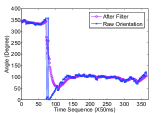
(a) Turning

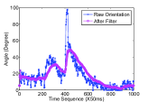
(b) Changing Lane

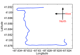
(c) Driving Trace

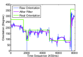
(d) Estimated Orientation

Figure 5: Turning or changing lanes, and Driving Trace

Turning: Sometimes, vehicles may turn at intersections, which could be detected by sensors. Figure 4(b) indicates the centripetal force sensed by the accelerometer, and the scale of the acceleration depends on the speed at which the vehicle is turning. Simultaneously, the angular velocity sensed by the gyroscope also reaches up to $0.5$ rad/s in our test case (Figure 4(c)), and the data from the magnetometer changes as well with a large fluctuation. Finally, the orientation of the smartphone also changes approximately $90$ degrees when turning left or right. Such angle change is observed along the axis in gravity direction, and the reading $0$, $90$, $180$, $270$ represent north, east, south, and west respectively. Although the angle may not be accurate enough due to the large noise in the magnetometer (the maximum error we experienced was approximately $30^{o}$), we are still able to correctly determine the road segment to which the car is turning by calibration. For example, Fig. 5(a) shows a case when vehicle turns from the north, the angle is from about $350^{o}$ to $100^{o}$, which is east. We also compare the measured angle differences for turning and lane changing (Figure 5(b)) since lane changing can be wrongly detected as a turning. In fact, the angle difference when a car changes its lane is much smaller than the one when a car make a turn. In addition, we also calculated the standard deviation for the angle differences in lane changing, which is less than $10$. Thus, distinguishing the turning and the lane changing is feasible. Then, we conduct more studies on the driving orientation estimation. Figure 5(c) plots the raw trace of the vehicle achieved from the GPS with good signals, and Figure 5(d) illustrates the raw orientation generated only by the inertial sensors. We employ moving average to cancel some noises and calculate the driving orientation, which matches the ground truth.

Other possible road infrastructures that a vehicle may experiences are bridges, and tunnels. In our measurement, such patterns are more obvious and easier to be detected, mainly reflected in acceleration along the gravity direction, where the reading experiences a large and fluctuation when driving in a uphill or a downhill, as shown in Figure 4(e).

In fact, certain driving patterns, such as turing left or right and stopping for traffic lights or stop signs, can be more accurately detected and thus classified. To classify other road infrastructures, we collect sensor readings of those patterns as the fingerprints, and then match the real-time sensor readings with the trained fingerprints. To improve the classification and the matching accuracy, we rely on the coarse-grained estimation of the location from dead-reckoning first, and then we further use our predictive regression model (Section V) to confine the search space: only the road infrastructures (stored fingerprints) $I$ within a certain distance $\delta$ from the estimated location $x$ will be considered as the matching candidate for the real-time pattern $P$ achieved from the sensory data. We select the infrastructure that maximizes the weighted matching score:

$$\alpha M(I,P)+(1-\alpha)e^{-D(x,L(I))}$$

where $M(I,P)$ is the matching score between the fingerprint of an infrastructure $I$ and the observed pattern $P$, $\alpha\in(0,1)$ is a constant, and $D(x,L(I))$ is the geodesic distance between the location $x$ and the location $L(I)$ of infrastructure $I$. Then, the estimated location $x$ is updated as the location $L(I^{*})$ of the infrastructure $I^{*}$ which maximizes the weighted matching score.

VII Experiments and Evaluations

We conduct extensive evaluation of SmartLoc in two different scenarios, both in downtown Chicago and suburb highways. We test the performance in highways to evaluate the effectiveness and reliability of SmartLoc replacing traditional GPS localization, so that it could save energy in navigation process. In our evaluation, Samsung Galaxy S3 is mounted to the windshield, and we drive for over $100$ different road segments in downtown Chicago ranging from $1$km to $10$kms and over $30$kms in highway. Since the inertial sensors provide the driving orientation, combined with driving distance from the location in last timeslot, the real-time location could be obtained. Thus, the key problem becomes estimating the trajectory distance. We evaluate the traveling distance, road infrastructure recognition, accuracy, and energy consumption.

VII-A Trajectory Distance Estimation

In trajectory distance estimation, we denote the trajectory distance in a timeslot as a traveling segment. Since the typical frequency for reliable GPS update in a smartphone (0.5Hz) is much lower than that of the sensors (1Hz-20Hz), we take duration for reliable GPS updating period as s timeslot. We focus on the evaluation of the trajectory distance estimation in two aspects: (1) the accuracy in distance estimating in traveling segment; and (2) the accuracy in final distance estimation of longer road segments. Then, we analyze the performance in details in the rest of the section.

VII-A1 Prediction in City Without Using Landmarks

We first test SmartLoc in downtown Chicago for over $30$ different roads, where some roads have reliable GPS signals and some not. We separate these roads into more than $100$ road segments, whose sizes are determined by our evaluations presented in the rest of the section. Before we describe the performance of SmartLoc in metropolises, we have to admit that the GPS signals in downtown Chicago are relatively poor and time dependent. Therefore, it is difficult to obtain the ground truth of all locations using smartphones, even if we adopt WiFi or GSM, fine grained location information are also hard to get. In this case, we adopt the experiment in some areas with accuracy locations getting from GPS, and we remove some of the GPS information in these areas to simulate the missing good signal. And we apply SmartLoc to calculate the location in those removed road segments to compare with the ground truth. Similarly, we analyze the performance of SmartLoc in two phases as aforementioned.

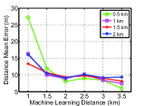
(a) Mean error in each slot

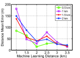
(b) Mean overall distance error

Figure 6: Accuracy vs. Learning Distance.

Obviously, the driving habits and road conditions in a city are difficult to predict, and slight deceleration makes the predicted result deviate from the ground truth. We first evaluate the reliability of SmartLoc when different driving distances are used to train the system, ranging from $0.5$km to $3.5$km. Generally speaking, the accuracy increases when the learning distance increases as illustrated in Figure 6(a). In this figure, the X axis indicates the driving distance used for training our predictive regression model, and the Y axis represents the mean distance (between the actual location reported by the GPS and the location estimated by our SmartLoc) in every timeslot when we update GPS locations (i.e., every 2 seconds, or about every $22$m when driving at the speed $40$km/h). This experiment measures the accuracy of the prediction when we drive for over four different road segments with length from $0.5$km to $2$km ($24$ different cases in total). Due to the unstable driving activities, short road segments for training SmartLoc leads to a large estimation error in each time slot. When SmartLoc learns only using the trace of $1$km, the mean error in every time slot in different scenarios is around $15$ meters, and the largest one is nearly $30$ meters. When SmartLoc trains our predictive regression model using a longer trace, the mean estimation error decreases in all the test cases. The smallest error is less than $6$m, which is less than half of the error when the training trace is $1$km. We also observe that the error grows with the increase of the length of the test road segment in most scenarios. For example, by training SmartLoc using a trace of $3.5$km, the mean error of the estimation in a $2$km road segment is nearly twice of that when testing a $0.5$km road segment.

We then evaluate the error on estimating the overall trajectory distance (Figure 6(b)) all the road segments and measure the error between the predicted distance and the ground truth distance for each segment (of all segments with distance from $0.5$km to $2$km) under different training traces. If SmartLoc learns the model for only 1km, the parameters in Eq. (2) cannot be computed accurately enough. Thus, the estimation errors increase to $180$m in all our tests. When SmartLoc learns enough samples, the parameters are much more reliable, and the average accumulated error is far below $30$m, which is significantly better than the GPS in Chicago downtown.

VII-A2 Prediction in City Using Landmarks

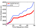
(a) Sensors Only

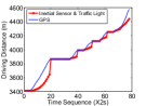
(b) Sensors and Traffic Lights

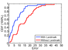
(c) Landmark vs No-Landmark

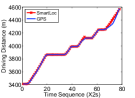
(d) SmartLoc

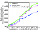
(e) Overall Comparison

Figure 7: Distance prediction comparison among three methods and ground truth.

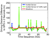
(a) Error of driving distance in every time slot for three methods

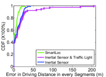
(b) Error of driving distance in every time slot for three methods

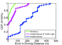
(c) Error of long distance estimation for three methods

Figure 8: Comparison of three methods.

SmartLoc calibrates the location as soon as it detects specific patterns, especially traffic lights and turnings. We test the performance of SmartLoc in a real drive route with the calibration using landmarks, and the result is presented as Figure 9,

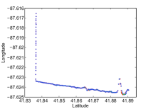
Figure 9: Localization In the Street.

which is a bird’s-eye view of the driving trajectory. The blue dots are the ground truth samples that we achieved from the GPS (where the GPS signals are good), the red dots are the predicted locations from our SmartLoc with all calibration techniques, and the length of green lines denote the dimension of error. In this figure, most of the red dots and blue dots are overlap with each other, which reflect the high accuracy in real downtown scenario.

We then compare the performance of three different methods in detail: using inertial sensors only, using sensors and landmark calibration, and using SmartLoc with all learning model and calibration. In this experiment, we assume the first $3400$m is with reliable GPS signals, and the precise locations are accessible. The estimation starts from $3400$m, and the first three figures in Figure 7 indicate the driving distance from the starting point versus the elapsed time.

In Figure 7(a), we conducted the experiment based on sensors only, without any calibration or noise canceling. The double integration on acceleration leads to the final deviation of over $400$m after driving about $1200$m. When the road pattern detection is introduced, the location is calibrated when SmartLoc senses the road infrastructure pattern. During the same experiment, our vehicle crossed $5$ traffic lights in total, and successfully detected all 5 traffic lights. The estimated locations are all then adjusted accordingly. The error in Figure 7(b) is still high, especially in the crossroads. Surprisingly, after combining our predictive regression model, SmartLoc’s result almost coincides with the ground truth, as shown in Figure 7(d). For the first $900$m, the curve of SmartLoc nearly overlaps with the curve of the ground truth. For the first $450$m, the vehicle passes three crossroads with all green lights, and the error is less than $20$m in most of the time. After the final traffic lights, the vehicle has to drive at a relatively low speed because of the road construction. The predicted distance consequently deviates from the ground truth a little, but at the end of the road, the errors remain small. We plot all the estimated distances by three methods in Figure 7(e), with the X axis being the ground truth distance and Y axis being the predicted distance, i.e., the perfect prediction will have a diagonal line. SmartLoc results are distributed almost along the diagonal line, and pure sensor approach deviates greatly.

The deviation of the results from the ground truth comes from the accumulated errors from all time slots. Based on the previous experiments, we plot the error in every time slot in Figure 8(a). SmartLoc with landmarks calibration has the smallest mean error of the estimated locations for all time slots: $90\%$ of them are lower than $20$m from the CDF in Figure 8(b). The other two approaches have larger errors, and the last figure describes the CDF of the total driving distance error.

VII-A3 Prediction in Highway

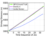
(a) Traveling Distance

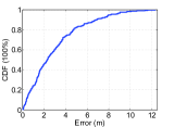
(b) Absolute error

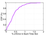
(c) Relative error

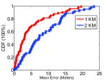
(d) Long Distance Estimation

Figure 10: Traveling in a highway.

In addition, we test the performance of SmartLoc on the highway to evaluate the probability of replacing traditional GPS to save energy. In the highway, GPS signals are almost always good, so the GPS data served as the ground truth only in this evaluation.

We drive over $10$ different highway segments with total distance being over $60$km (with driving speed $100$km/h-$120$km/h approximately). The smartphone has access to the precise location information from the GPS, which is updated every $2$ seconds. Meanwhile, we collect the readings from the sensors and train our predictive regression model for $3$km. Then, we predict the traveling distance for the next $2$km and compare the distances from the ground truth, SmartLoc and the pure sensors.

Figure 10(a) illustrates the comparisons of driving distance estimation using SmartLoc (with sensors) and the GPS. The ground truth (GPS readings) is plotted by the green curve. It is obvious that the error between pure sensor-based solution and the ground truth is becoming larger along the time, which is due to the accumulated errors without any calibration. By using our predictive regression model, SmartLoc calculate suitable parameters and apply them into the prediction. The estimation errors gets much smaller after then. Figure 10(b) indicates that the largest error is only $12$m among the $10$ different highway segments (each of length $2$km), and in over $80\%$ cases, the errors are less than $5$m. Compared with the actual distance extracted from the ground truth (Figure 10(c)), at over $95\%$ locations (among all locations where GPS location can be extracted), the errors are less than $1\%$ of the actual driving distance, and the largest error is less than $2\%$ of the actual driving distance. We also notice that the accuracy of the prediction decreases with the increase of the driving distance. We predict the driving distance for both $1$km and $2$km after taking the data of the first $3$km to build the model. In our experiments, $80\%$ of the prediction error for both (1km) and (2km) cases are less than $10$m and $15$m respectively, and even the largest error fall within $19.8m$ and $23m$ as plotted in Figure 10(d).

However, based on the evaluation, we discover that the estimation results cannot maintain high accuracies for a long distance even in highway. The main reason comes from the user dependent driving behaviors and the unpredictable special conditions, such as traffic jam. We also consider that SmartLoc has a better estimation accuracy when the driving speeds remain stable, and when the driving speed fluctuates frequently, the error of SmartLoc’s predicted results still in an acceptable range. Calibrating the location periodically is a feasible way to improve the location accuracy in real life applications, which is also an alternative to replace traditional GPS to save energy in the highway.

VII-A4 Evaluations Analysis

Based on the evaluation results presented in this section, an obvious conclusion is that SmartLoc provides precise driving distance estimation in certain scenarios. In every time slot, the driving distance is estimated from the current sensor data as well as our predictive regression model. Suppose the error (denoted as $D_{i}$) in the estimation of each time slot $i$ follows normal distribution: $D_{i}\sim{\mathcal{N}(\mu,\sigma^{2})}$, with mean $\mu$ and variance $\sigma^{2}$. Then, the estimation of the total traveling distance $S_{t}$ in $t$ timeslots is the summation of the traveling distance in all time slots: $S_{t}={\displaystyle\sum\limits_{i=1}^{t}D_{i}}$. In this case, the error, from a long term perspective, will be accumulated. Obviously, $S_{t}\sim{\mathcal{N}(t\mu,t\sigma^{2})}$. The variance of the variable $S_{t}$ will be $t\sigma^{2}$. Thus, the mean error increases along the time, which leads to the conclusion that it is difficult to predict the traveling distance precisely in a long term, although sometimes the deviation in some continuous timeslots may be neutralized. For a given error bound $\delta$, $Pr(S_{t}\geq\delta)$ is higher when $t$ is larger.

VII-B Localization in the City

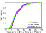
(a) Error of location estimation in every sampling timeslot

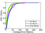
(b) Error in locating the final destination in different blocks

Figure 11: Navigation performance evaluation.

We then present the localization results in Chicago downtown. As aforementioned, it is difficult to get the ground truth for the majority of the sampling locations.

We set the experiments of estimating the final location. Since, Section III has demonstrated that there are $9$ bad road segments with lengths over $400$m, which is less than $3$ blocks in downtown Chicago. The goal of SmartLoc is then to obtain a relatively accurate distance estimation within three blocks. We randomly select $100$ points as destinations in the experiment, and a destination could be one block, two blocks, or three blocks away from the starting point. We drive to these destination points to evaluate if the destination is precisely calculated by SmartLoc. We assume that the GPS signals are good before the starting point, and SmartLoc will train the dead-reckoning model during the driving. In this experiment, we test the accuracy of estimating the traveling distance in every time slot and of estimating the overall driving distance (i.e., locating the final destination) as shown in Figure 11(a) and Figure 11(b) respectively. When SmartLoc only navigates to the destination within one block, with probability $70\%$, the error of estimating the location for each sampling slot is less than $10$m, and with probability $85\%$, the mean error is less than $30$m. When the destination is two blocks away, about $75\%$ of the errors are less than $30$m; when the destination is three blocks away, about $80\%$ errors are less than $50$m. From these figures, the error of destination locating within a few blocks is acceptable. We also plot the localization results for one road segment with length over $6400$m in Figure 9. In this figure, the red spots denote the ground truth generated from GPS, and the blue spots represent the localization calculated by SmartLoc, where the green line between them is the localization error for every location.

VIII Conclusion

This paper presented SmartLoc, a metropolis localization system by using the inertial sensors and the GPS module of smartphones. We established a predictive regression model to estimate the trajectory using linear regression, and the proposed SmartLoc detects the road infrastructures and driving patterns as landmarks to calibrate the localization results. Our extensive evaluations shows that SmartLoc improves the localization accuracy to less than $20m$ for more than $90\%$ roads in Chicago downtown, compared with $\geq 50\%$ with raw GPS data.

References

- [1] Skyhook. http://www.skyhookwireless.com/.
- [2] Chen, M., Sohn, T., Chmelev, D., Haehnel, D., Hightower, J., Hughes, J., LaMarca, A., Potter, F., Smith, I., and Varshavsky, A. Practical metropolitan-scale positioning for gsm phones. UbiComp (2006), 225–242.
- [3] Chen, W., Fu, Z., Chen, R., Chen, Y., Andrei, O., Kroger, T., and Wang, J. An integrated gps and multi-sensor pedestrian positioning system for 3d urban navigation. In JURSE (2009), IEEE, pp. 1–6.
- [4] Cheng, Y., Chawathe, Y., LaMarca, A., and Krumm, J. Accuracy characterization for metropolitan-scale wi-fi localization. In MobiSys (2005), ACM, pp. 233–245.
- [5] Constandache, I., Choudhury, R., and Rhee, I. Towards mobile phone localization without war-driving. In INFOCOM, 2010 Proceedings IEEE (2010), IEEE, pp. 1–9.
- [6] Enge, P., and Van Dierendonck, A. Wide area augmentation system. Progress in Astronautics and Aeronautics 164 (1996), 117–142.
- [7] Eriksson, J., Girod, L., Hull, B., Newton, R., Madden, S., and Balakrishnan, H. The pothole patrol: using a mobile sensor network for road surface monitoring. In ACM MobiSys (2008).
- [8] Griswold, W., Shanahan, P., Brown, S., Boyer, R., Ratto, M., Shapiro, R., and Truong, T. Activecampus: experiments in community-oriented ubiquitous computing. Computer 37, 10 (2004), 73–81.
- [9] Guha, S., Plarre, K., Lissner, D., Mitra, S., Krishna, B., Dutta, P., and Kumar, S. Autowitness: locating and tracking stolen property while tolerating gps and radio outages. In SenSys (2010), ACM, pp. 29–42.
- [10] Hu, S., Su, L., Liu, H., Wang, H., and Abdelzaher, T. Smartroad: a crowd-sourced traffic regulator detection and identification system. In IPSN (2013), ACM, pp. 331–332.
- [11] Hwang, S., and Yu, D. Gps localization improvement of smartphones using built-in sensors.
- [12] Jirawimut, R., Ptasinski, P., Garaj, V., Cecelja, F., and Balachandran, W. A method for dead reckoning parameter correction in pedestrian navigation system. Instrumentation and Measurement 52, 1 (2003), 209–215.
- [13] Levi, R., and Judd, T. Dead reckoning navigational system using accelerometer to measure foot impacts, Dec. 10 1996. US Patent 5,583,776.
- [14] Liu, H., Gan, Y., Yang, J., Sidhom, S., Wang, Y., Chen, Y., and Ye, F. Push the limit of wifi based localization for smartphones. In MobiCom (2012), ACM, pp. 305–316.
- [15] Liu, J., Priyantha, B., Hart, T., Ramos, H., Loureiro, A., and Wang, Q. Energy efficient gps sensing with cloud offloading.
- [16] Mohan, P., Padmanabhan, V., and Ramjee, R. Nericell: rich monitoring of road and traffic conditions using mobile smartphones. In SenSys (2008), ACM, pp. 323–336.
- [17] Newson, P., and Krumm, J. Hidden markov map matching through noise and sparseness. In GIS (2009), ACM, pp. 336–343.
- [18] Obradovic, D., Lenz, H., and Schupfner, M. Fusion of map and sensor data in a modern car navigation system. Journal of VLSI signal processing systems 45, 1-2 (2006), 111–122.
- [19] Ojeda, L., and Borenstein, J. Non-gps navigation with the personal dead-reckoning system. In Defense and Security Symposium (2007).
- [20] Paek, J., Kim, J., and Govindan, R. Energy-efficient rate-adaptive gps-based positioning for smartphones. In MobiSys (2010), ACM, pp. 299–314.
- [21] Parkinson, B., and Enge, P. Differential gps. Global Positioning System: Theory and applications. 2 (1996), 3–50.
- [22] Rai, A., Chintalapudi, K., Padmanabhan, V., and Sen, R. Zee: Zero-effort crowdsourcing for indoor localization. In MobiCom (2012), ACM, pp. 293–304.
- [23] Retscher, G. An intelligent multi-sensor system for pedestrian navigation. Journal of Global Positioning Systems 5, 1-2 (2006), 110–118.
- [24] Thiagarajan, A., Ravindranath, L., Balakrishnan, H., Madden, S., Girod, L., et al. Accurate, low-energy trajectory mapping for mobile devices. In NSDI (2011), USENIX Association, pp. 20–20.
- [25] Thiagarajan, A., Ravindranath, L., LaCurts, K., Madden, S., Balakrishnan, H., Toledo, S., and Eriksson, J. Vtrack: accurate, energy-aware road traffic delay estimation using mobile phones. In SenSys (2009), ACM, pp. 85–98.
- [26] Titterton, D., Weston, J., Titterton, D., and Weston, J. Strapdown inertial navigation technology. Institution of Electrical Engineers.
- [27] Varshavsky, A., Chen, M., de Lara, E., Froehlich, J., Haehnel, D., Hightower, J., LaMarca, A., Potter, F., Sohn, T., Tang, K., et al. Are gsm phones the solution for localization? In WMCSA (2006), IEEE, pp. 34–42.
- [28] Wang, H., Sen, S., Elgohary, A., Farid, M., Youssef, M., and Choudhury, R. No need to war-drive: Unsupervised indoor localization. In MobiSys (2012), ACM, pp. 197–210.
- [29] Woodman, O., and Harle, R. Pedestrian localization for indoor environments. In Ubicomp (2008), ACM, pp. 114–123.
- [30] Yang, Z., Wu, C., and Liu, Y. Locating in fingerprint space: wireless indoor localization with little human intervention. In MobiCom (2012), ACM, pp. 269–280.
- [31] Yuan, J., Zheng, Y., Zhang, C., Xie, X., and Sun, G.-Z. An interactive-voting based map matching algorithm. In MDM (2010), IEEE, pp. 43–52.