Claw-free $t$-perfect graphs can be recognised in polynomial time

Abstract

A graph is called $t$-perfect if its stable set polytope is defined by non-negativity, edge and odd-cycle inequalities. We show that it can be decided in polynomial time whether a given claw-free graph is $t$-perfect.

1 Introduction

We treat $t$-perfect graphs, a class of graphs that is not only similar in name to perfect graphs but also shares a number of their properties. One way to define perfect graphs is via the stable set polytope: The convex hull of all characteristic vectors of stable sets (sets of pairwise non-adjacent vertices). As shown independently by Chvátal [6] and Padberg [21], a graph is perfect if and only if its stable set polytope is determined by non-negativity and clique inequalities. In analogy, Chvátal [6] proposed to study the class of graphs whose stable set polytope is defined by non-negativity, edge and odd-cycle inequalities. These graphs became to be known as $t$-perfect graphs. (We defer precise and more explicit definitions to the next section.)

Two celebrated results on perfect graphs are the proof of the strong perfect graph conjecture by Chudnovsky, Robertson, Seymour and Thomas [5] and the polynomial time algorithm of Chudnovsky, Cornuéjols, Liu, Seymour and Vušković [4] that checks whether a given graph is perfect or not. Analogous results for $t$-perfection seem desirable but out of reach for the moment. Restricted to claw-free graphs, however, this changes. A characterisation of claw-free $t$-perfect graphs in terms of forbidden substructures was recently proved by Bruhn and Stein [3]. In this work we present a recognition algorithm for $t$-perfect claw-free graphs:

Theorem 1.

It can be decided in polynomial time whether a given claw-free graph is $t$-perfect.

The class of $t$-perfect graphs seems rich and of non-trivial structure. Examples include series-parallel graphs (Boulala and Uhry [1]) and bipartite or almost bipartite graphs. More classes were identified by Shepherd [26] and Gerards and Shepherd [12]. An attractive result on the algorithmic side is the combinatorial polynomial-time algorithm of Eisenbrand, Funke, Garg and Könemann [9] that solves the max-weight stable set problem on $t$-perfect graphs.

There is also an, at least superficially, more stringent notion of $t$-perfection, strong $t$-perfection; see Schrijver [25, Vol. B, Ch. 68] where also some background on $t$-perfect graphs may be found. Interestingly, there is no $t$-perfect graph known that fails to be strongly $t$-perfect. In fact, for some classes these two notions are known to be equivalent, see Schrijver [24] and Bruhn and Stein [2].

The graphs whose stable set polytope is given by non-negativity, clique and odd-cycle inequalities are called $h$-perfect. The class of $h$-perfect graphs is a natural superclass of both perfect as well as $t$-perfect graphs. The class has been studied by Fonlupt and Uhry [11], Sbihi and Uhry [23], and Király and Páp [18, 19].

We briefly outline the strategy of our recognition algorithm. In Sections 3 and 4, we show how to recognise $t$-perfect line graphs. For this, we work in the underlying source graph that gives rise to the line graph. In the source graph we need to detect certain subgraphs called thetas: two vertices joined by three disjoint paths. In the thetas that are of interest to us the linking paths have to respect additional parity constraints.

The general algorithm for claw-free graphs is presented in Sections 5 and 6 and relies on a divide and conquer approach to split the input graph along small separators. In this phase of the algorithm, we make extensive use of a procedure by van ’t Hof, Kamiński and Paulusma [28] that detects induced paths of given parity in claw-free graphs. The final pieces that cannot be split anymore turn out to be essentially line graphs, which we already dealt with.

2 Claw-free graphs and $t$-perfection

We refer to Diestel [8] for general notation and definitions concerning graphs.

Let us recall the definition of a claw-free graph. The claw is the graph $G=(V,E)$ with $V=\{u,v_{1},v_{2},v_{3}\}$ and $E=\{uv_{1},uv_{2},uv_{3}\}$, and we call $u$ its centre. A graph is called claw-free if it does not contain an induced subgraph that is isomorphic to the claw. Claw-free graphs form a superclass of line graphs.

In order to define $t$-perfection, we associate with every graph $G=(V,E)$ a polytope denoted TSTAB$(G)$, the set of all vectors $x\in\mathbb{R}^{V}$ satisfying

$$0\leq x_{v}\leq 1 \text{ for every vertex }v\in V,$$

$$x_{u}+x_{v}\leq 1 \text{ for every edge }uv\in E,$$ (1)

$$\sum_{v\in V(C)}x_{v}\leq\lfloor\tfrac{1}{2}|V(C)|\rfloor \text{ for every odd cycle }C\text{ in }G.$$

The graph $G$ is called $t$-perfect if TSTAB$(G)$ coincides with the stable set polytope of $G$ (the convex hull of characteristic vectors of stable sets in $\mathbb{R}^{V}$). An alternative but equivalent definition is to say that $G$ is $t$-perfect if and only if TSTAB$(G)$ is an integral polytope.

As observed by Gerards and Shepherd [12], the following operation called $t$-contraction preserves $t$-perfection: Contraction of all edges incident with any vertex $v$ whose neighbourhood $N(v)$ is a stable set. We then say that a $t$-contraction is performed at $v$. If $G$ is claw-free, the $t$-contraction becomes particularly simple. Indeed, a $t$-contraction at $v$ is only possible if $v$ has degree $\leq 2$; otherwise $v$ is the centre of a claw. If $v$ has precisely two neighbours $u$ and $w$ then the $t$-contraction simply identifies $u,v,w$ to a single vertex.

To characterise the class of $t$-perfect graphs in terms of forbidden substructures, the concept of $t$-minors was introduced in [2]: A graph $H$ is a $t$-minor of a graph $G$ if $H$ can be obtained from $G$ by a series of vertex deletions and/or $t$-contractions. Note that the class of $t$-perfect graphs is closed under taking $t$-minors.

We note an easy but useful observation [2]:

any $$t$$-minor of a claw-free graph is claw-free. (2)

It turns out that $t$-perfect claw-free graphs can be characterised in terms of finitely many forbidden $t$-minors:

Theorem 2 (Bruhn and Stein [3]).

A claw-free graph is $t$-perfect if and only if it does not contain any of $K_{4}$, $W_{5}$, $C^{2}_{7}$ and $C^{2}_{10}$ as a $t$-minor.

Here, $K_{4}$ denotes the complete graph on four vertices, $W_{5}$ is the $5$-wheel, and for $n\in\mathbb{N}$ we denote by $C^{2}_{n}$ the square of the cycle $C_{n}$ on $n$ vertices, see Figure 1. More precisely, we define $C^{2}_{n}$ always on the vertex set $v_{1},\ldots,v_{n}$, so that $v_{i}$ and $v_{j}$ are adjacent if and only if $|i-j|\leq 2$, where we take the indices modulo $n$.

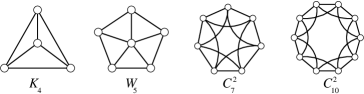
Figure 1: The forbidden $t$-minors.

We often present our algorithms intermingled with parts of the corresponding correctness proofs. To set the algorithm steps apart from the surrounding proofs we write them as follows:

1. The first line of an algorithm.

Finally, for two vertices $u,v$, a $u$–$v$-path is simply a path from $u$ to $v$. Similarly, if $X,Y\subseteq V(G)$, then we mean by an $X$–$Y$-path a path from a vertex in $X$ to some vertex in $Y$ so that no internal vertex belongs to $X\cup Y$. In the case that $X=Y$ we simply speak of an $X$-path.

3 Line graphs

We first solve the recognition problem for line graphs:

Lemma 3.

It can be decided in polynomial time whether the line graph of a given graph is $t$-perfect.

We develop the algorithm in the course of this section and the next. That the algorithm is correct is based on the following characterisation of $t$-perfect line graphs.

We call a graph subcubic if its maximum degree is at most 3. A skewed theta is a subgraph which is the union of three edge-disjoint paths linking two vertices, called branch vertices, such that two paths have odd length and one has even length. Note that a skewed theta does not have to be an induced subgraph.

Lemma 4.

[3] Let $G$ be a graph. Then the line graph $L(G)$ is $t$-perfect if and only if $G$ is subcubic and does not contain any skewed theta.

Checking for subdivisions of a certain graph can often be reduced to the well-known $k$-Disjoint Paths problem: Given a number of $k$ pairs of terminal vertices, the task is to decide whether there are disjoint paths joining the paired terminals. In our context, however, this is not sufficient as the paths linking the branch vertices in a skewed theta are subject to parity constraints.

That this deep and seemingly hard problem, $k$-Disjoint Paths with Parity Constraints, allows nevertheless a polynomial time algorithm has been announced by Kawarabayashi, Reed and Wollan [17]. Another algorithm was given in the PhD thesis of Huynh [14]. These are very impressive results indeed, and they draw on deep insights coming from the graph minor project of Robertson and Seymour and its extension to matroids by Geelen, Gerards and Whittle. For both algorithms, however, it seems doubtful whether they could be implemented with a reasonable amount of work (or at all). We prefer therefore to present a more elementary algorithm for Lemma 3 that does not rely on any deep result and that is, in principle, implementable.

Given a bipartition $\mathcal{P}=(A,B)$ (where we allow $A$ or $B$ to be empty) of the vertex set of a graph $G$, we call an edge $\mathcal{P}$-even if its endvertices lie in distinct partition classes of $\mathcal{P}$; otherwise the edge is $\mathcal{P}$-odd. We observe that a cycle is odd if and only if it contains an odd number of $\mathcal{P}$-odd edges.

The algorithm we present here to check for skewed thetas runs in two phases. We start with any bipartition $\mathcal{P}$. In the first phase, the algorithm tries to iteratively reduce the number of $\mathcal{P}$-odd edges. If this is no longer possible we either have found a skewed theta or we have arrived at a bipartition $\mathcal{P}^{\prime}$ with at most two $\mathcal{P}^{\prime}$-odd edges. Then, in the second phase, we exploit that any skewed theta has to contain at least one of the at most two $\mathcal{P}^{\prime}$-odd edges. In that case, it becomes possible to check directly for a skewed theta:

Lemma 5.

Given a graph $G$ and a bipartition $\mathcal{P}$ of $V(G)$ so that at most two edges are $\mathcal{P}$-odd, it is possible to check in polynomial time whether $G$ contains a skewed theta.

The proof of Lemma 5 is deferred to Section 4. In the remainder of this section, we show how to iteratively reduce the number of $\mathcal{P}$-odd edges. We start with two lemmas that give sufficient conditions for the existence of a skewed theta.

Lemma 6.

A $2$-connected subcubic graph that contains two edge-disjoint odd cycles contains a skewed theta.

Proof.

Let $C_{1}$ and $C_{2}$ be two edge-disjoint odd cycles in $G$, which then are also vertex-disjoint as the graph is assumed to be subcubic. Since $G$ is $2$-connected there are two disjoint $C_{1}$–$C_{2}$-paths $P_{1},P_{2}$. The endvertices of $P_{1}$ and $P_{2}$ subdivide $C_{2}$ into two subpaths, and one of these subpaths together with $P_{1}$ and $P_{2}$ yields an odd $C_{1}$-path, and thus a skewed theta. ∎

For any bipartition $\mathcal{P}$ of $G$ define $G_{\mathcal{P}}$ to be the (bipartite) subgraph on $V(G)$ together with all the $\mathcal{P}$-even edges. We formulate a second set of conditions that implies the presence of a skewed theta.

Let $C$ be a cycle and let $P$ and $Q$ be two disjoint $C$-paths. Let $p_{1},p_{2}$ be the endpoints of $P$ and $q_{1},q_{2}$ be the endpoints of $Q$. We say that $P$ and $Q$ are crossing on $C$ if $p_{1},q_{1},p_{2},q_{2}$ appear in this order on $C$.

Lemma 7.

Let $G$ be a subcubic graph with a bipartition $\mathcal{P}$. Let there be three $\mathcal{P}$-odd edges $o_{1},o_{2},o_{3}$ and two disjoint trees $T_{1},T_{2}\subseteq G_{\mathcal{P}}$, each containing an endvertex of each of $o_{1},o_{2},o_{3}$.

Assume the trees are minimal subject to the above description. If $G_{\mathcal{P}}$ contains three edge-disjoint $T_{1}$–$T_{2}$-paths then $G$ contains a skewed theta.

Proof.

Throughout the proof, we assume that $G$ does not contain a skewed theta. Our aim is to show that $G_{\mathcal{P}}$ does not contain three edge-disjoint $T_{1}$–$T_{2}$-paths.

For this, we first prove a sequence of more general claims. Let $r_{1}r_{2}$ and $s_{1}s_{2}$ be two $\mathcal{P}$-odd edges of $G$ such that there are two disjoint paths $R_{1}=r_{1}\ldots s_{1}$, $R_{2}=r_{2}\ldots s_{2}$. Let $C$ be the cycle $r_{1}R_{1}s_{1}s_{2}R_{2}r_{2}r_{1}$.

We claim that

any two edge-disjoint $$R_{1} R_{2} P,Q C$$–-paths are crossing on . (3)

If $P$ and $Q$ are not crossing then we can easily find two edge-disjoint cycles in $R_{1}\cup R_{2}\cup P\cup Q$, one through $r_{1}r_{2}$ and the other through $s_{1}s_{2}$. By Lemma 6, however, this is impossible. Thus, $P$ and $Q$ are crossing.

Next, we show that

the endvertices of any two edge-disjoint $$R_{1} R_{2} P,Q R_{1} \mathcal{P}$$–-paths in lie in distinct partitions classes of . (4)

Denote the endvertex of $P$ in $R_{1}$ by $p_{1}$ and denote the one in $R_{2}$ by $p_{2}$; define $q_{1},q_{2}$ analogously for $Q$.

Suppose that $p_{1}$ and $q_{1}$ lie in the same partition class of $\mathcal{P}$. Since $G$ is subcubic, $P$ and $Q$ are disjoint, and, by (3), crossing. Assume that $p_{1}\in r_{1}R_{1}q_{1}$. As $p_{1}$ and $q_{1}$ are contained in the same partition class, the path $p_{1}R_{1}q_{1}$ has even length. On the other hand, the following two paths have odd length: $p_{1}Pp_{2}R_{2}s_{2}s_{1}R_{1}q_{1}$ and $q_{1}Qq_{2}R_{2}r_{2}r_{1}R_{1}p_{1}$. As, moreover, these three paths meet only in $p_{1}$ and $q_{1}$ we have found a skewed theta; this proves (4).

From this follows that

$$G R_{1} R_{2}$$ cannot contain three edge-disjoint –-paths. (5)

Indeed, by (4), the three endvertices of such paths in $R_{1}$ would need to lie in distinct partition classes, which is clearly impossible as $\mathcal{P}$ is a bipartition.

To complete the proof, suppose now that $G_{\mathcal{P}}$ contains three edge-disjoint $T_{1}$–$T_{2}$-paths $P_{1},P_{2},P_{3}$. Denote by $t_{i}$ the unique vertex that separates all the endvertices of $o_{1},o_{2},o_{3}$ in $T_{i}$ (unless $T_{i}$ is a path this is the vertex of degree $3$ in $T_{i}$). Observe that $t_{i}$ subdivides $T_{i}$ into three edge-disjoint paths $S^{i}_{1},S^{i}_{2},S^{i}_{3}$ (some of which might be trivial) so that $S^{i}_{j}$ contains the endvertex of $o_{j}$ (for $i=1,2$ and $j=1,2,3$).

Pick two distinct $k,\ell\in\{1,2,3\}$ so that for $i=1,2$ at least two paths in $P_{1},P_{2},P_{3}$ the endvertex in $T_{i}$ is contained in $S^{i}_{k}\cup S^{i}_{\ell}=:R_{i}$. Let $\{m\}=\{1,2,3\}\setminus\{k,\ell\}$. Should now $P_{j}$ have its endvertex $p$ in $S^{1}_{m}-S^{1}_{k}-S^{1}_{\ell}$ concatenate the subpath $pS^{1}_{m}t_{1}$ with $P_{j}$, and proceed in a similar way in $T_{2}$. In this way we turn the edge-disjoint $T_{1}$–$T_{2}$-paths into edge-disjoint $R_{1}$–$R_{2}$-paths. Now, we obtain the desired contradiction from (5). ∎

Next, we state a simple lemma that, however, is the key to reducing the number of $\mathcal{P}$-odd edges.

Lemma 8.

Let $G$ be a graph with a bipartition $\mathcal{P}$. Given an edge-cut $F$ of $G$ that contains more $\mathcal{P}$-odd edges than $\mathcal{P}$-even edges, one can compute a bipartition $\mathcal{P}^{\prime}$ of $G$ with less $\mathcal{P}^{\prime}$-odd edges in polynomial time.

Proof.

Let $F=E(X,Y)$ separate $X\subseteq V(G)$ from $Y\subseteq V(G)$ in $G$. Then put $\mathcal{P}^{\prime}:=(A\triangle X,B\triangle X)$, and observe that every $\mathcal{P}$-odd edge in $F$ becomes $\mathcal{P}^{\prime}$-even, while the edges outside $F$ do not change. ∎

Putting together the lemmas presented so far, we arrive at the following procedure.

Lemma 9.

There is a polynomial-time algorithm that takes as input a $2$-connected subcubic graph $G$, a bipartition $\mathcal{P}$ and three $\mathcal{P}$-odd edges $o_{1},o_{2},o_{3}$. The algorithm:

1. either correctly decides that $G$ contains a skewed theta;

2. or computes an edge cut $F$ that contains more $\mathcal{P}$-odd edges than $\mathcal{P}$-even edges.

Proof.

We describe the algorithm in the course of this lemma. We omit a detailed discussion about the runtime complexity as the steps of the algorithm rely on basic operations or reduce to solving min-cut/max-flow problems.

1. If $G_{\mathcal{P}}$ is not connected, choose a component $X$ of $G_{\mathcal{P}}$ and return $F=E(X,G-X)$. enumerate Since $G$ is $2$-connected, $F$ contains at least two $\mathcal{P}$-odd edges, which is condition (b). Let us now assume that $G_{\mathcal{P}}$ is connected. enumerate

2. Compute a spanning tree $T$ of $G_{\mathcal{P}}$ and determine the fundamental cycles $C_{o_{1}},C_{o_{2}},C_{o_{3}}$ of $o_{1},o_{2},o_{3}$.

3. If any two of $C_{o_{1}},C_{o_{2}}$ and $C_{o_{3}}$ are edge-disjoint, return “skewed theta”. enumerate

   The return value in line❿ is justified by Lemma 6, which means that we may assume the cycles $C_{o_{1}},C_{o_{2}},C_{o_{3}}$ to pairwise share an edge from now on. enumerate

4. If there is an edge $e$ shared by each of $C_{o_{1}},C_{o_{2}},C_{o_{3}}$:

   1. Let $T_{1}$ and $T_{2}$ be the two components of $\bigcup_{i=1}^{3}C_{o_{i}}-e$.

   2. Delete leaves from $T_{1}$ and $T_{2}$ until $T_{1}$ and $T_{2}$ have the form of Lemma 7.

   3. Compute a smallest cut $F^{\prime}=E_{G_{\mathcal{P}}}(X,Y)$ of $G_{\mathcal{P}}$ that separates $T_{1}$ from $T_{2}$

   4. If $|F^{\prime}|\geq 3$, return “skewed theta”; otherwise return $F=E_{G}(X,Y)$.

   enumerate Note that, for $i=1,2,3$, both components of $C_{o_{i}}-\{e,o_{i}\}$ contain an endvertex of $o_{i}$, so that, after pruning, $T_{1}$ and $T_{2}$ indeed conform with Lemma 7. Lemma 7 implies that $G$ contains a skewed theta if $|F^{\prime}|\geq 3$. Otherwise, $F$ contains at most two $\mathcal{P}$-even edges and the three $\mathcal{P}$-odd edges $o_{1},o_{2},o_{3}$.

   Considering line❿, we may from now on assume that there is no common edge of $C_{o_{1}},C_{o_{2}},C_{o_{3}}$. Then

   there is a unique cycle $$D \bigcup_{i=1}^{3}C_{o_{i}} o_{1},o_{2},o_{3} G_{\mathcal{P}} D-\{o_{1},o_{2},o_{3}\}$$ in that passes through each of and so that there is a path in between any two of the components of that avoids the third. (6)

   Indeed, each $C_{o_{i}}-o_{i}$ is a subpath of $T$ and families of subtrees of a tree are known to have the Helly property, that is, if any two share a vertex then there is also a common vertex to all. Let $x$ be such a vertex. Now, assume that $C_{o_{1}},C_{o_{2}},C_{o_{3}}$ do not have a common edge. Note that, for any $i\neq j$, $C_{o_{i}}$ and $C_{o_{j}}$ meet along a path. It follows that $C_{o_{1}}\cup C_{o_{2}}\cup C_{o_{3}}$ decomposes into a cycle $D$ that passes through all of $o_{1},o_{2},o_{3}$ and three internally disjoint $x$–$D$-paths that each end in a different component of $D-\{o_{1},o_{2},o_{3}\}$. Uniqueness of $D$ follows from the fact that $\bigcup_{i=1}^{3}C_{o_{i}}-\{o_{1},o_{2},o_{3}\}$ is a tree. This proves (6).

   enumerate

5. Determine the cycle $D$ in $\bigcup_{i=1}^{3}C_{o_{i}}$ that passes through $o_{1},o_{2}$ and $o_{3}$. enumerate Finding $D$ is easy, as this is done in the tree $\bigcup_{i=1}^{3}C_{o_{i}}-\{o_{1},o_{2},o_{3}\}$. (Alternatively, we may argue that $E(D)$ is exactly the set of those edges in $\bigcup_{i=1}^{3}C_{o_{i}}$ that lie in only one of the cycles $C_{o_{i}}$.) Let $S_{1},S_{2},S_{3}$ be the three components of $D-\{o_{1},o_{2},o_{3}\}$.

   enumerate

6. Check whether there is a single edge $e^{\prime}$ that separates $S_{1}$ from $S_{2}\cup S_{3}$ in $G_{\mathcal{P}}$. If yes, return $E_{G}(X,Y)$, where $X$ and $Y$ are the two components of $G_{\mathcal{P}}-e^{\prime}$. enumerate Two of the edges $o_{1},o_{2},o_{3}$ are in the cut $E_{G}(X,Y)$, while the only $\mathcal{P}$-even edge in it is $e^{\prime}$.

   enumerate

7. Compute two edge-disjoint $S_{1}$–$(S_{2}\cup S_{3})$-paths $P,Q$ in $G_{\mathcal{P}}$ so that one ends in $S_{2}$ and the other in $S_{3}$. enumerate Let us explain how $P$ and $Q$ can be computed. First, we use a standard algorithm to find two edge-disjoint $S_{1}$–$(S_{2}\cup S_{3})$-paths $P,Q$ in $G_{\mathcal{P}}$; these exist by Menger’s theorem and line❿. If already one ends in $S_{2}$ and the other in $S_{3}$, we use these. So, assume that $P$ and $Q$ both end in $S_{2}$, say. By (6), we can find an $S_{1}$–$S_{3}$-path $R$ in $G_{\mathcal{P}}-S_{2}$. If $R$ is disjoint from $P$ and $Q$, we replace $Q$ by $R$. If not, we follow $R$ until we encounter for the last time a vertex of $P\cup Q$, where we see $R$ directed from $S_{1}$ to $S_{3}$. Let us say this last vertex $q$ is in $Q$. Then, we replace $Q$ by $QqR$.

   enumerate

8. If $P$ and $Q$ are not crossing on $D$ then return “skewed theta”.

9. Otherwise, choose an edge $e^{\prime\prime}$ that separates the endvertices of $P$ and $Q$ in $S_{1}$ and apply lines 4b–4d to the two components $T_{1}$ and $T_{2}$ of $(D-\{o_{1},o_{2},o_{3},e^{\prime\prime}\})\cup P\cup Q$.

If $P$ and $Q$ are not crossing then $D\cup P\cup Q$ contains two disjoint odd cycles, and thus $G$ contains a skewed theta, by Lemma 6. If, on the other hand, $P$ and $Q$ are crossing then each of the two components $T_{1}$ and $T_{2}$ as in line❿ is incident with an endvertex of each of $o_{1},o_{2},o_{3}$. ∎

We now prove that for line graphs $t$-perfection can be checked in polynomial-time.

Proof of Lemma 3..

Let $G$ be a given graph. If $G$ has maximum degree at least $4$, its line graph $L(G)$ is not $t$-perfect by Lemma 4. Otherwise, we apply the algorithm below to the blocks of $G$ to check whether $G$ contains a skewed theta. Clearly, any skewed theta is completely contained in a block of $G$.

1. Set $\mathcal{P}:=(V(G),\emptyset)$.

2. While there are at least $2$ distinct $\mathcal{P}$-odd edges, do the following:

   1. Run the algorithm of Lemma 9.

   2. If the algorithm returns a cut $F=E_{G}(X,Y)$ with more $\mathcal{P}$-odd edges than $\mathcal{P}$-even edges, apply Lemma 8.

3. Apply Lemma 5 to decide whether $G$ contains a skewed theta.

The algorithm runs in polynomial-time, as the number of $\mathcal{P}$-odd edges decreases in each iteration of the while loop.

Correctness holds as Lemma 4 guarantees that $L(G)$ is $t$-perfect if and only if $G$ does not contain a skewed theta. ∎

4 Proof of Lemma 5

After having reduced the number of $\mathcal{P}$-odd edges, we are in this section in the situation that at most two remain. We note that, in this setting, checking for a skewed theta can be reduced to several applications of $k$-Disjoint Paths with a $k$ of at most $5$. For any fixed $k$ a polynomial time algorithm is known to exist, see for instance Kawarabayashi, Kobayashi and Reed [15]. However, there does not seem to be a practical algorithm known if $k\geq 3$.

We therefore give here an algorithm for Lemma 5 that only relies on the solution of $2$-Disjoint Paths, for which several explicit algorithms are known that are independent of the heavy machinery of the graph minor project. We start by treating the case when there is only one odd edge.

Lemma 10.

Let $G$ be a subcubic graph with a bipartition $\mathcal{P}$ such that there is at most one $\mathcal{P}$-odd edge. Then it can be decided in polynomial time whether $G$ has a skewed theta.

Proof.

If $G$ does not have any $\mathcal{P}$-odd edge then it cannot contain a skewed theta, and if $G$ is not $2$-connected then any skewed theta lies in the block that contains the $\mathcal{P}$-odd edge. Thus, we may assume that the input graph $G$ is $2$-connected and contains a unique $\mathcal{P}$-odd edge, $xy$ say. Let $\mathcal{P}=(A,B)$, and let $x,y\in A$.

1. If $|V(G)|\leq 3$, return “no skewed theta”. enumerate

   We perform, if possible, one of two reductions in order to make the instance size smaller. If both $x$ and $y$ are of degree $2$, then we add an edge between the neighbour $x^{\prime}\neq y$ of $x$ and the neighbour $y^{\prime}\neq x$ of $y$, and we delete $x,y$. See Figure 2 (a) for an illustration. (Observe that $x^{\prime}\neq y^{\prime}$, as $G$ is not a triangle.) Denoting the resulting graph by $\tilde{G}$ and the induced bipartition by $\mathcal{\tilde{P}}$, we note that the only $\mathcal{\tilde{P}}$-odd edge of $\tilde{G}$ is $x^{\prime}y^{\prime}$. Moreover, $\tilde{G}$ has a skewed theta if and only if $G$ has a skewed theta.

   

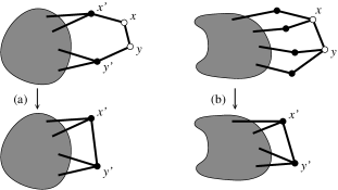
   Figure 2: Reduction $G\to\tilde{G}$

   In a similar way, we perform a reduction when both $x$ and $y$ have degree $3$, and if each neighbour $u\notin\{x,y\}$ of $x$ or of $y$ has degree $2$. Then we identify $x$ and $N(x)-y$ to a new vertex $x^{\prime}$, and $y$ and $N(y)-x$ to a new vertex $y^{\prime}$; see Figure 2 (b). Again, the resulting graph $\tilde{G}$ has a skewed theta precisely when $G$ has one; and the only $\mathcal{\tilde{P}}$-odd edge is $x^{\prime}y^{\prime}$. enumerate

2. As long as possible, successively reduce $G$ to $\tilde{G}$. enumerate By exchanging $x$ and $y$, if necessary, we may therefore assume that

   $$x u,v\neq y \deg_{G}(y)=3 \deg_{G}(u)=3$$ has two neighbours , and if then as well. (7)

   The algorithm proceeds with enumerate

3. Check whether $G$ contains a skewed theta, in which $x$ is a branch vertex. enumerate This is the case if and only if there is a vertex $z\in B$ such that there are three paths between $z$ and $\{y,u,v\}$ that have pairwise only $z$ in common. Clearly, this can be checked for in polynomial time.

   enumerate

4. If $G-x$ is $2$-connected return “skewed theta”. enumerate If $G-x$ is $2$-connected, then there is a cycle $C$ through $y$ and some other neighbour of $x$, say $u$. Since $x\in A$ and thus $u\in B$, it follows that both paths from $y$ to $u$ in $C$ are of odd length. Now, $C$ together with the path $yxu$ forms a skewed theta.

   So, we may assume that $G-x$ has cutvertices: Let their union with $N_{G}(x)$ be denoted with $S$. Note that line❿ implies that any skewed theta in $G$ has its two branch vertices in a common non-trivial block of $G-x$. We prove:

   every block of $$G-x S X_{*} S$$ contains exactly two vertices of , except for possibly one block, denoted by , that contains three vertices of . (8)

   To prove the claim, consider the graph $H$ obtained from $G-x$ by adding three new vertices $p_{1},p_{2},p_{3}$ each of which is precisely adjacent to a distinct neighbour of $x$. Then the cutvertices of $H$ are exactly the vertices in $S$. Consider the block tree of $H$, that is, the graph defined on the blocks and cutvertices, where a block $X$ and a cutvertex $w$ are adjacent if $w\in V(X)$. Then, as $G$ is $2$-connected every leaf in the block tree contains one of $p_{1},p_{2},p_{3}$. Thus, the block tree has at most (in fact, precisely) three leaves, which directly gives Claim (8).

   We use the following observation.

   if any non-trivial block $$X G-x S \mathcal{P} G$$ of contains two vertices of in distinct classes of  then contains a skewed theta. (9)

   Suppose that (9) is false. Let $y^{\prime}$ be a vertex of $S\cap V(X)$ for which there is a $y^{\prime}$–$y$-path $P_{y}$ that is internally disjoint from $X$. Now, as (9) is false there is a vertex $z\in S\cap V(X)$ so that $y^{\prime}$ and $z$ are not in the same bipartition class of $\mathcal{P}$. As $z\in S$, there is a path $P_{z}$ from $z$ to one of $u,v$, $u$ say, that is internally disjoint from $X$. Let $C$ be a cycle in $X$ that contains $y^{\prime}$ and $z$. Then $C\cup P_{y}\cup P_{z}$ together with $uxy$ is a skewed theta with branch vertices $y^{\prime},z$. This proves (9).

   enumerate

5. Compute the block decomposition of $G-x$, and check for (9). enumerate

   For every non-trivial block $X$ of $G-x$ we now construct a new graph $X^{\prime}$, so that

   $$G X X^{\prime}$$ has a skewed theta both of whose branch vertices are contained in if and only if has a skewed theta. (10)

   Moreover, the bipartition $\mathcal{P}$ extends in a natural way to $X^{\prime}$ so that there is precisely one $\mathcal{P}$-odd edge in $X^{\prime}$. The construction is sketched in Figure 3.

   First consider a non-trivial block $X$ that contains exactly two vertices of $S$, say $r$ and $s$. We observe that there is an $r$–$s$-path $P$ in $G$ that is internally disjoint from $X$ and that passes through $xy$. As $r$ and $s$ are in the same class of $\mathcal{P}$, the path $P$ has odd length. We set $X^{\prime}:=X+rs$. Clearly, any skewed theta of $X^{\prime}$ contains $rs$. By replacing $rs$ with $P$, we then obtain a skewed theta of $G$. Conversely, a skewed theta of $G$ with both branch vertices in $X$ has a subpath from $r$ to $s$ that passes through $xy$. Substituting this subpath by $rs$ yields a skewed theta of $X^{\prime}$. Thus, we see that (10) is satisfied.

   

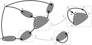
   Figure 3: The reduction of the blocks

   Second, we treat the unique block $X_{*}$ containing three vertices of $S$, if there is such a block. Let the three vertices of $S$ in $X_{*}$ be $u^{\prime},v^{\prime},y^{\prime}$, where the names are chosen such that there are disjoint paths $P_{u},P_{v},P_{y}$ linking $u$ to $u^{\prime}$, $v$ to $v^{\prime}$ and $y$ to $y^{\prime}$, and so that each of these paths is internally disjoint from $X_{*}$.

   We claim that

   $$\{u^{\prime},v^{\prime},y^{\prime}\}\subseteq A$$. (11)

   Indeed, since we already checked for (9), either all of $\{u^{\prime},v^{\prime},y^{\prime}\}$ are contained in $A$ or in $B$. So, suppose that $\{u^{\prime},v^{\prime},y^{\prime}\}\subseteq B$. Now we find three internally disjoint paths between $y^{\prime}$ and $x$, which means that $x$ is a branch vertex of a skewed theta. This, however, is impossible by (3). To obtain the paths, start with the three paths $xyP_{y}y^{\prime}$, $xuP_{u}u^{\prime}$ and $xvP_{v}v^{\prime}$, and extend the two latter paths by internally disjoint $\{u^{\prime},v^{\prime}\}$–$y^{\prime}$-paths in $X_{*}$. These exists, since $X_{*}$ is a non-trivial block. This proves (11).

   We let now $X_{*}^{\prime}$ be the graph obtained from $X_{*}$ by adding $x,u,v$ and the edges $xy^{\prime},uu^{\prime},vv^{\prime}$. (Note, that $y=y^{\prime}$ is possible, while $u,v\in B$ always implies $u\neq u^{\prime}$ and $v\neq v^{\prime}$.) With this, (10) is satisfied.

   enumerate

6. Compute for every block $X$ of $G-x$ the graph $X^{\prime}$ and apply line❿ to every $X^{\prime}$ independently. enumerate

   In order to bound the total number of recursions called, we observe that

   $$|V(X^{\prime})|<|V(G)| X G-x \sum_{X}|V(X^{\prime})|\leq|V(G)|+2$$ for every non-trivial block of , and , where the sum ranges over the non-trivial blocks. (12)

   Indeed, the second claim is immediate as $G$ is subcubic, which is maintained throughout the algorithm, implies that no two non-trivial blocks of $G-x$ share a vertex. The only vertices that may appear in two $X_{1}^{\prime},X_{2}^{\prime}$ are $u,v$, and then only if one of $X_{1},X_{2}$ is equal to $X_{*}$. The first claim needs only proof for $X_{*}$.

   So, suppose that $|V(X_{*}^{\prime})|=|V(G)|$. Since in constructing $X_{*}^{\prime}$ we add to $X_{*}$ the three vertices $x,u,v$, this is only possible if $y\in V(X_{*})$, that is, if $y=y^{\prime}$. Then, since $X_{*}$ is a non-trivial block but $y$ is adjacent to $x\notin V(X_{*})$, we deduce that $\deg_{G}(y)=3$, which by (7) gives $\deg_{G}(u)=3$ as well. If $u$ had two of its neighbours in $X_{*}$ then $u$ itself would be contained in $X_{*}$, which is impossible as then $u=u^{\prime}\in A$, by (11), but $x\in A$ implies $u\in B$. Thus, $u$ has besides $x$ a second neighbour outside $X_{*}$, which then also lies outside $X_{*}^{\prime}$. This shows that $|V(X_{*}^{\prime})|<|V(G)|$.

   Using a standard analysis of the recurrence relation given by (12), we get that the total number of recursions is $\mathcal{O}(|V(G)|^{2})$. Indeed, the input graph is split up into, essentially, disjoint parts, each of which is properly smaller than $G$. ∎

   Lemma 11.

   There is a polynomial-time algorithm that, given a $2$-connected subcubic graph $G$ and given a bipartition $\mathcal{P}$ of its vertex set so that there are exactly two $\mathcal{P}$-odd edges $o_{1},o_{2}$, either

   1. decides correctly that $G$ has a skewed theta;

   2. or computes a minimal cut $F$ containing $o_{1},o_{2}$ and at most two other edges.

   Proof.

   Since the algorithm below can be reduced to min cut/max-flow problems, it clearly can be implemented to run in polynomial time.

   1. Compute two disjoint paths $P_{1},P_{2}$, each of which linking one endvertex of $o_{1}$ to one endvertex of $o_{2}$.

   2. Compute a minimal cut $F$ in $G$ separating $P_{1}$ from $P_{2}$.

   3. If $|F|\leq 4$, return $F$.

   4. If $|F|\geq 5$, return “skewed theta”.

   For the proof of correctness, observe first that paths $P_{1},P_{2}$ as in line❿ exists as $G$ is $2$-connected. Moreover, $F$ contains $o_{1},o_{2}$. Thus, if $|F|\leq 4$ we have indeed outcome (6a). So, suppose that $|F|=5$, which implies that there is a set $\mathcal{Q}$ of three edge-disjoint $P_{1}$–$P_{2}$-paths. From $\Delta(G)\leq 3$ it follows that the paths in $\mathcal{Q}$ are, in fact, pairwise disjoint. Now, if any two of them are not crossing on the cycle $C:=P_{1}\cup P_{2}+o_{1}+o_{2}$ then $G$ contains two odd disjoint cycles and therefore a skewed theta, by Lemma 6. So, we may assume that any two of them cross on $C$.

   We observe that two of the paths in $\mathcal{Q}$, let us say $R,S$, have their endvertices on $P_{1}$ in the same class of $\mathcal{P}$. Let the endvertices of $R$ be $r_{1}$ and $r_{2}$, and $s_{1}$ and $s_{2}$ those of $S$, where $r_{1}$ and $s_{1}$ lie in $P_{1}$. Then deletion of the internal vertices of $r_{2}P_{2}s_{2}$ from $C\cup R\cup S$ yields a skewed theta with $r_{1},s_{1}$ as branch vertices. ∎

   Lemma 12.

   There is a polynomial-time algorithm that, given a subcubic graph $G$ with a bipartition $\mathcal{P}$ of its vertex set so that there are exactly two $\mathcal{P}$-odd edges $o_{1},o_{2}$ and given a minimal cut $F$ containing $o_{1},o_{2}$ and at most two other edges, decides whether $G$ has a skewed theta.

   Proof.

   We first reduce to the relevant blocks of the graph.

   1. If the $\mathcal{P}$-odd edges are in separate blocks, apply Lemma 10 to both blocks in order to decide whether $G$ contains a skewed theta.

   2. If both edges are in a single block, say $B$, set $G:=B$ and continue. enumerate So we may assume that $G$ is 2-connected. Next we try to find an even smaller cut containing $o_{1},o_{2}$. enumerate

   3. Check whether there is an edge $e$, so that $\{o_{1},o_{2},e\}$ is a cut, and if yes, apply Lemma 8 to $F^{\prime}=\{o_{1},o_{2},e\}$ and then Lemma 10 in order to decide whether $G$ contains a skewed theta. enumerate We allow here that $e\in\{o_{1},o_{2}\}$. From line❿ follows, in particular, that $|F|=4$, say $F=\{o_{1},o_{2},e_{1},e_{2}\}$. enumerate

   4. Apply Lemma 10 to $G-o_{1}$ and to $G-o_{2}$.

   5. Apply Lemma 8 and then Lemma 10 to $G-e_{1}$ and to $G-e_{2}$. enumerate Since $F$ is minimal, there are two components $C_{1}$, $C_{2}$ of $G-F$. After lines❿ and❿, we are sure that

      any skewed theta of $$G F C_{1} C_{2}$$ contains every edge of . In particular, both branch vertices either lie in or in . (13)

      We know from Lemma 6 that two disjoint odd cycles imply the presence of a skewed theta. As we have only two $\mathcal{P}$-odd edges, the problem reduces here to the $2$-Disjoint Paths problem, which may be handled, for example, with the algorithm of Tholey [27]. enumerate

   6. Check whether $G$ contains two disjoint odd cycles, and if yes return “skewed theta”. enumerate Next, we prove that

      for $$i=1,2 C_{i} P_{i}=x_{i}\ldots u_{i} Q_{i}=y_{i}\ldots v_{i} x_{i},y_{i} o_{1},o_{2} u_{i},v_{i} e_{1},e_{2}$$, in there are internally disjoint paths and , where are distinct endvertices of and are distinct endvertices of . (14)

      Indeed, suppose that there are no such paths in $C_{1}$, say. As $G$ is subcubic, there are then also no two such paths that are merely edge-disjoint rather than vertex-disjoint. Moreover, because $C_{1}$ is connected and $G$ subcubic, no three edges of $o_{1},o_{2},e_{1},e_{2}$ can have the same endvertex. Thus there is an edge $e$ that separates in $C_{1}$ the endvertices of $o_{1},o_{2}$ from the endvertices of $e_{1},e_{2}$. Consequently, $\{o_{1},o_{2},e\}$ is a cut of $G$, which is a case we had already discarded in line❿.

      enumerate

   7. Compute $P_{i},Q_{i}$ as in (14). enumerate As $G$ does not contain any two disjoint odd cycles, we may assume that

      $$o_{1}=x_{1}x_{2},\,o_{2}=y_{1}y_{2},\,e_{1}=v_{1}u_{2}\text{\em and }e_{2}=u_{1}v_{2}.$$

      See Figure 4 for these edges. Using again the fact that $G$ does not possess any two disjoint odd cycles, we may deduce that

      for $$i=1,2 C_{i} y_{i} u_{i} x_{i} v_{i}$$, there are no two disjoint paths in linking to and to . (15)

      In the remainder of the proof, we compute two subcubic graphs $G_{1}$ and $G_{2}$ such that

      $$G G_{1} G_{2}$$ contains a skewed theta if and only if or does. (16)

      Moreover, the restriction of $\mathcal{P}$ to $V(G_{i})$ gives a bipartition $\mathcal{P}_{i}$ of $G_{i}$ with two $\mathcal{P}_{i}$-odd edges.

      We only describe the construction of $G_{1}$; $G_{2}$ is obtained by reversing the sides $C_{1}$ and $C_{2}$. We define a path $P_{2}^{\prime}$ that is used to replace the path $x_{1}x_{2}P_{2}u_{2}v_{1}$ in $G_{1}$. If $P_{2}$ has odd length, we set $P^{\prime}_{2}:=x_{1}v_{1}$. By considering the bipartition classes of $\mathcal{P}$, we may see that $x_{1}\neq v_{1}$ and that the resulting new edge $x_{1}v_{1}$ is a $\mathcal{P}_{1}$-odd edge. On the other hand, if $P_{2}$ has even length we set $P^{\prime}_{2}:=x_{1}x_{2}v_{1}$. Note that in both cases the path $P^{\prime}_{2}$ has the same parity as the path $x_{1}x_{2}P_{2}u_{2}v_{1}$ in $G$. We define $Q_{2}^{\prime}$ analogously and set $G_{1}:=C_{1}\cup P^{\prime}_{2}\cup Q^{\prime}_{2}$.

      

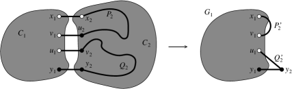
      Figure 4: Construction of $G_{1}$ if $P_{2}$ has odd length and $Q_{2}$ even length

      We note that for $i=1,2$

      $$|E(G_{i})|<|E(G)|,\,\Delta(G_{i})\leq 3\text{\em and }|E(G_{1})|+|E(G_{2})|\leq|E(G)|+4.$$ (17)

      While the last two inequalities should be clear, the first needs proof. As $G$ is subcubic but $|F|=4$, we deduce that $C_{2}$ has at least two vertices. As, on the other hand, $C_{2}$ is connected we see that $C_{2}$ contains at least one edge. That edge, however, is missing in $G_{1}$, which implies $|E(G_{1})|<|E(G)|$. The proof for $G_{2}$ is the same.

      To prove (16), we first assume that $G$ contains a skewed theta $T$. By (13), $T$ has its two branch vertices $r,s$ either in $C_{1}$ or in $C_{2}$, let us say that $r,s\in V(C_{1})$. Moreover, each of the two odd paths of $T$ between $r$ and $s$ passes through exactly one of $o_{1},o_{2}$. Thus, the two odd paths contain subpaths $R,S\subseteq C_{2}$ linking $\{x_{2},y_{2}\}$ to $\{u_{2},v_{2}\}$ in $C_{2}$. From (15) it follows that one of $R$ and $S$, $R$ say, starts in $x_{2}$ and ends in $u_{2}$, while the other, $S$ in this case, connects $y_{2}$ to $v_{2}$. Since the parity of the length of $R$ is determined by the classes of $\mathcal{P}$ that contain $x_{2}$ and $u_{2}$, it follows that the parity of the length of $R$ is the same as that of $P_{2}$, which is the same as that of $P^{\prime}_{2}$. Since the same reasoning holds for $S$ and $Q^{\prime}_{2}$, we see that we obtain a skewed theta of $G_{1}$ from $T$ by replacing $x_{1}x_{2}Ru_{2}v_{1}$ by $P^{\prime}_{2}$ and $y_{1}y_{2}Sv_{2}u_{1}$ by $Q^{\prime}_{2}$.

      For the other direction, observe that any skewed theta of $G_{1}$ contains at least one of $P^{\prime}_{2}$ and $Q^{\prime}_{2}$ (in fact both, but we do not need that observation). By replacing, if necessary, $P^{\prime}_{2}$ by $x_{1}x_{2}P_{2}u_{2}v_{1}$ and/or $Q^{\prime}_{2}$ by $y_{1}y_{2}Q_{2}v_{2}u_{1}$, we turn the skewed theta of $G_{1}$ into one of $G$.

      enumerate

   8. Compute $G_{1}$ and $G_{2}$ and re-apply the algorithm to $G_{1}$ and $G_{2}$.

   Correctness of the algorithm follows from (16). It remains to analyse the running time of the algorithm. Each line can be performed in polynomial time, so it suffices to bound the recursion. Here, (17) shows that the graph is split into two parts which are properly smaller and, essentially, disjoint. A standard analysis of the recurrence relation shows that the total number of recursions called is $\mathcal{O}(|E(G)|^{2})$. ∎

   Proof of Lemma 5..

   The algorithm performs the following steps.

   1. If $G$ is not 2-connected, compute the blocks of $G$ and re-apply the algorithm to each block separately.

   2. If $G$ does not have any $\mathcal{P}$-odd edge, return “no skewed theta”.

   3. If $G$ has a single $\mathcal{P}$-odd edge, apply Lemma 10 to decide whether $G$ has a skewed theta.

   4. If $G$ has two $\mathcal{P}$-odd edges, apply Lemma 11 to $G$, to compute the promised cut $F$. Then apply Lemma 12 to decide whether $G$ has a skewed theta.

   Correctness and polynomial running time follow from the respective lemmas. ∎

   5 Claw-free graphs

   We now describe an algorithm that, given a claw-free graph $G$, decides in polynomial time whether $G$ is $t$-perfect or not. We present the algorithm in a number of steps over the course of this section. First, we use that we can already decide $t$-perfection for line graphs, and that we can detect whether a graph is a line graph efficiently:

   Theorem 13 (Roussopoulos [22]).

   It can be checked in linear time whether a given graph is a line graph. Moreover, given a line graph $G$, a graph $H$ with $L(H)=G$ can be found in linear time.

   Thus, the first step in the algorithm becomes:

   1. Use Theorem 13 to check whether $G$ is a line graph. If yes, compute $H$ with $L(H)=G$ and apply the algorithm of Lemma 3 to $H$. If no, proceed to the next line below. enumerate Next, we observe that we can assume the input graph to be $2$-connected. For this, we say that a pair $(G_{1},G_{2})$ of proper induced subgraphs of a graph $G$ is a separation of $G$, if $G=G_{1}\cup G_{2}$. The order of the separation is equal to $|V(G_{1}\cap G_{2})|$.

      The following lemma may be deduced directly from the definition of $t$-perfection. We only apply it to claw-free graphs, where it becomes a simple consequence of Theorem 2.

      Lemma 14.

      Let $(G_{1},G_{2})$ be a separation of a graph $G$ so that $G_{1}\cap G_{2}$ is complete. Then $G$ is $t$-perfect if and only if $G_{1}$ and $G_{2}$ are $t$-perfect.

      enumerate

   2. Determine the blocks of $G$, and apply the rest of the algorithm to each block independently. Return “not $t$-perfect” if one of the blocks is not $t$-perfect; otherwise return “$t$-perfect”. enumerate Clearly, this step can be performed efficiently, and is, by Lemma 14, correct. Thus, we may from now on assume $G$ to be $2$-connected. Moreover, it is easy to see that $G$ is not $t$-perfect, if it contains a vertex of degree at least $5$. Indeed, as $G$ is claw-free, the neighbourhood of any vertex $v$ of degree at least $5$ always contains either a triangle or an induced $5$-cycle. In the former case, the graph contains a $K_{4}$ and in the latter case a $5$-wheel as induced subgraph.

      enumerate

   3. If $\Delta(G)\geq 5$ or if $G\in\{C^{2}_{7},C^{2}_{10}\}$ return “not $t$-perfect”.

   4. If $G\in\{C^{2}_{6}-v_{1}v_{6},C^{2}_{7}-v_{7},C^{2}_{10}-v_{10}\}$ return “$t$-perfect”. enumerate That the three graphs in line❿ are $t$-perfect is proved in [3]. (In fact, $C_{7}^{2}$ and $C_{10}^{2}$ are minimally $t$-imperfect, that is, they are $t$-imperfect but every proper $t$-minor is $t$-perfect. The graph $C^{2}_{6}-v_{1}v_{6}$ can be seen to be a $t$-minor of $C_{10}^{2}$.)

      The remainder of the algorithm is based on the following lemma.

      Lemma 15 (Bruhn and Stein [3]).

      Let $G$ be a $3$-connected claw-free graph of maximum degree at most $4$. If $G$ does not contain $K_{4}$ as $t$-minor then one of the following statements holds true:

      1. $G$ is a line graph; or

      2. $G\in\{C^{2}_{6}-v_{1}v_{6},C^{2}_{7}-v_{7},C^{2}_{10}-v_{10},C^{2}_{7},C^{2}_{10}\}$.

      Thus, we may assume that the input graph $G$ is $2$-connected but not $3$-connected. That is, $G$ has a separation of order $2$. enumerate

   5. If $G$ is $3$-connected, return “not $t$-perfect”.

   6. Otherwise, find a separation $(G_{1},G_{2})$ of $G$ of order $2$. Let $u,v$ be the two vertices in $G_{1}\cap G_{2}$. enumerate Line❿ is correct, as we had already excluded that $G$ is a line graph, nor one of the exceptional graphs in (b) of Lemma 15.

      To continue, we use a result that allows us to reduce the $t$-perfection of $G$ to the $t$-perfection of the two sides of the separation. For this, we write $G_{i}/_{u=v}$ for the graph obtained from $G_{i}$ by identifying $u$ and $v$.

      Lemma 16.

      Let $G$ be a $2$-connected claw-free graph of maximum degree at most $4$. Assume $(G_{1},G_{2})$ to be a separation of $G$ with $V(G_{1}\cap G_{2})=\{u,v\}$. Then:

      1. If $G_{1}$ and $G_{2}$ each contain induced $u$–$v$-paths of both even and odd length, then $G$ is not $t$-perfect.

      Otherwise $G$ is $t$-perfect if and only if $\tilde{G}_{1}$ and $\tilde{G}_{2}$ are $t$-perfect, where

      1. $\tilde{G}_{1}=G_{1}/_{u=v}$ and $\tilde{G}_{2}=G_{2}+uv$, if $G_{1}$ contains an odd induced $u$–$v$-path but $G_{2}$ does not;

      2. $\tilde{G}_{1}=G_{1}$ and $\tilde{G}_{2}=G_{2}$, if neither of $G_{1}$ and $G_{2}$ contains an odd induced $u$–$v$-path;

      3. $\tilde{G}_{1}=G_{1}+uv$ and $\tilde{G}_{2}=G_{2}/_{u=v}$, if $G_{1}$ contains an even induced $u$–$v$-path but $G_{2}$ does not; and

      4. $\tilde{G}_{1}=G_{1}$ and $\tilde{G}_{2}=G_{2}$, if neither of $G_{1}$ and $G_{2}$ contains an even induced $u$–$v$-path.

      We defer the proof of Lemma 16 to the next section. We combine the lemma with the following algorithm:

      Theorem 17 (van ’t Hof, Kamiński and Paulusma [28]).

      Given a claw-free graph $G$ and $u,v\in V(G)$, it can be decided in polynomial time whether there is an induced $u$–$v$-path of even (or of odd) length.

      With this, our algorithm continues as follows: enumerate

   7. Use Theorem 17 to determine the parities of induced $u$–$v$-paths in $G_{1}$ and in $G_{2}$.

   8. If $G_{1}$ and $G_{2}$ each contain induced $u$–$v$-paths of both even and odd length, return “not $t$-perfect”.

   9. Otherwise, choose $\tilde{G}_{1}$ and $\tilde{G}_{2}$ as in Lemma 16, and apply line❿ to $\tilde{G}_{1}$ and to $\tilde{G}_{2}$ independently. Return “$t$-perfect” if both are $t$-perfect, and “not $t$-perfect” otherwise.

   We can finally complete the proof of our main result, that $t$-perfection can be checked for in polynomial time if the input is restricted to claw-free graphs.

   Proof of Theorem 1.

   We have already seen that the algorithm described in the course of this section is correct. Moreover, as each single line is executed in polynomial time, we only need to bound the number of times each line is executed. For this, observe that every time there is a branching in line❿, the graph $\tilde{G}_{1}$ contains a vertex of $G$ that does not lie in $\tilde{G}_{2}$ and vice versa. Again, standard analysis of the recurrence yields that the number of iterations is bounded by $\mathcal{O}(|V(G)|^{2})$. ∎

   6 Proof of Lemma 16

   All that remains is Lemma 16. The first step in its proof consists of the observation that $t$-perfection in a claw-free graph depends essentially only on the existence of $K_{4}$ as a $t$-minor.

   Lemma 18.

   A connected claw-free graph $G$ is $t$-perfect if and only if

   1. $\Delta(G)\leq 4$;

   2. $G\neq C_{7}^{2}$ and $G\neq C^{2}_{10}$; and

   3. $G$ does not contain $K_{4}$ as a $t$-minor.

   Proof.

   We had already seen above that a $t$-perfect claw-free graph has maximum degree at most $4$. Thus, the forward direction is obvious. For the other direction assume $G$ to satisfy (i)–(iii) but suppose that $G$ is $t$-imperfect. By Theorem 2 and (iii), $G$ contains $W_{5}$, $C_{7}^{2}$ or $C_{10}^{2}$ as a proper $t$-minor.

   As $\Delta(G)\leq 4$ and since $G$ is connected, neither of $W_{5}$, $C_{7}^{2}$ or $C_{10}^{2}$ appears as induced subgraph in $G$. Thus, $G$ has a $t$-minor $H$ so that a single $t$-contraction in $H$ results in $W_{5}$, $C_{7}^{2}$ or $C_{10}^{2}$. We choose $H$ to have a minimum number of vertices.

   We first note that, by (2), the $t$-minor $H$ is still claw-free. Moreover, we deduce that $\Delta(H)\leq 4$. Indeed, suppose that $\Delta(H)\geq 5$. As $G$ does not contain $K_{4}$ as a $t$-minor, the same holds for $H$. In particular, no neighbourhood of any vertex of degree $\Delta(H)$ contains a triangle. So, it must contain $C_{5}$ as induced subgraph. As no $t$-contraction transforms $W_{5}$ into $W_{5}$, $C_{7}^{2}$ or $C_{10}^{2}$, this means in particular that $H$ contains $W_{5}$ as a proper induced subgraph, which in turn implies that $H$ was not minimum.

   Let us first consider the case when a single $t$-contraction of $H$ yields $C_{7}^{2}$. Since $H$ is claw-free, the $t$-contraction is performed at a vertex $v^{\prime\prime}_{1}$ with exactly two neighbours denoted with $v_{1}^{\prime}$ and $v^{\prime\prime\prime}_{1}$. We may assume that the resulting new vertex of the $t$-contraction is $v_{1}$ of $C_{7}^{2}$; see Figure 5.

   Figure 5: Examples of single $t$-contractions that yield $C^{2}_{7}$

   Now, as $v_{1}$ is adjacent to $v_{2},v_{3},v_{6},v_{7}$, it follows that $N_{H}(v_{1}^{\prime})\cup N_{H}(v_{1}^{\prime\prime\prime})=\{v_{2},v_{3},v_{6},v_{7}\}$. However, $v_{1}^{\prime}$ cannot have two non-adjacent neighbours $v_{i},v_{j}$ among $v_{2},v_{3},v_{6},v_{7}$, as that would result in a claw on $v_{i},v_{j},v_{1}^{\prime\prime}$ with centre $v_{1}^{\prime}$. As the same holds for $v_{1}^{\prime\prime\prime}$, it follows that one of $v_{1}^{\prime}$ and $v_{1}^{\prime\prime\prime}$ is adjacent to precisely $v_{2},v_{3}$ while the other has exactly $v_{6},v_{7}$ as neighbours among $v_{2},v_{3},v_{6},v_{7}$. If, however, $N_{H}(v_{1}^{\prime})=\{v_{1}^{\prime\prime},v_{6},v_{7}\}$ then $\{v_{7},v_{1}^{\prime},v_{2},v_{5}\}$ induces a claw in $H$, which is impossible.

   The case that $H$ can be $t$-contracted to $C_{10}^{2}$ is similar, so we skip to the case when $H$ contains $W_{5}$ as a $t$-contraction.

   Let $v$ be the vertex at which the $t$-contraction is performed, let $u,w$ be its two neighbours in $H$, and let $x$ be the resulting vertex in $W_{5}$, which needs to be the degree-$5$ vertex as $\Delta(H)\leq 4$. Then, one of $u,w$, let us say $u$, has at least three neighbours other than $v$. Since $H-\{u,v,w\}$ is a $5$-cycle, it follows that $u$ has at least two non-adjacent neighbours $y,z$ in $H-\{u,v,w\}$. But then $\{u,v,y,z\}$ induces a claw in $H$, a contradiction. This completes the proof. ∎

   In general, it is not entirely straightforward to describe the graphs from which $K_{4}$ can be obtained solely by $t$-contractions. For instance, Figure 6 shows two quite different graphs that both $t$-contract to $K_{4}$. In claw-free graphs, in contrast, there is only one such type of graph.

   

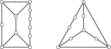
   Figure 6: Two graphs that $t$-contract to $K_{4}$

   A skewed prism (of a graph $G$) is an induced subgraph of $G$ that consists of two triangles, say $x_{1},x_{2},x_{3}$ and $y_{1},y_{2},y_{3}$, together with three vertex-disjoint induced paths $P_{1}$, $P_{2}$, and $P_{3}$, each of which has one endvertex in $x_{1},x_{2},x_{3}$ and the other in $y_{1},y_{2},y_{3}$. Moreover, we require the paths $P_{1}$ and $P_{2}$ to have even length, while $P_{3}$ has odd length. (We allow $P_{1}$ and $P_{2}$ to have length $0$.) As an illustration, note that the graph on the left in Figure 6 is a skewed prism but the one on the right is not (and it contains a claw).

   Let us stress the fact that, in contrast to the skewed thetas treated in Section 3, skewed prisms are induced subgraphs. Moreover, a skewed prism has two of its linking paths even and one odd, while for a skewed theta it is the opposite: two odd, one even. While this may create some confusion, we think that the name is nevertheless justified by the clear connection of skewed thetas and prisms: Indeed, the line graph of a skewed theta is a skewed prism, and moreover, a graph $G$ contains a skewed theta if and only if its line graph $L(G)$ contains a skewed prism.

   Lemma 19.

   A claw-free graph $G$ contains $K_{4}$ as a $t$-minor if and only if it contains a skewed prism.

   Proof.

   By successively $t$-contracting vertices of degree $2$, one obtains from any skewed prism a $K_{4}$. Thus, if $G$ contains a skewed prism, it contains $K_{4}$ as $t$-minor.

   For the other direction, let $H$ be a minimal induced subgraph of $G$ that can be $t$-contracted to $K_{4}$. Suppose that $H$ is not a skewed prism.

   Let $H_{0},H_{1},\ldots,H_{k}$ be a series of graphs with $H_{0}=H$ and $H_{k}\cong K_{4}$ such that $H_{i+1}$ is obtained from $H_{i}$ by a single $t$-contraction, for $i=0,\ldots,k-1$. Note that, as $H$ is minimal, no proper induced subgraph of $H_{i}$ contains $K_{4}$ as $t$-minor, for all $i=0,\ldots,k$.

   As $H_{k}\cong K_{4}$ is a skewed prism, there is an index $i\leq k-1$ such that $H_{i}$ is not a skewed prism but $H_{i+1}$ is. Let $H_{i+1}$ consist of the two triangles $x_{1},x_{2},x_{3}$ and $y_{1},y_{2},y_{3}$ and the disjoint $x_{i}$–$y_{i}$-paths $P_{i}$, for $i=1,2,3$, so that $P_{1},P_{2}$ have even length, while $P_{3}$ has odd length. Assume that the $t$-contraction occurs at a vertex $v$ of $H_{i}$, which then identifies its two neighbours $u,w$ to a new vertex $x$ of $H_{i+1}$.

   We first observe that the neighbourhoods of $u$ and $w$ in $H_{i}$ are incomparable: if, for example, $N_{H_{i}}(u)\subseteq N_{H_{i}}(w)$, then $H_{i+1}\cong H_{i}-\{u,v\}$, in contradiction to our observation that no proper induced subgraph of $H_{i}$ contains $K_{4}$ as $t$-minor. Similarly, $|N_{H_{i}}(u)|,|N_{H_{i}}(w)|\geq 2$.

   Let us discuss the case that $|N_{H_{i}}(u)|,|N_{H_{i}}(w)|\geq 3$. Since $H_{i}$ is claw-free, both $N_{H_{i}}(u)\setminus\{v\}$ and $N_{H_{i}}(w)\setminus\{v\}$ are cliques. This gives $|N_{H_{i}}(u)|,|N_{H_{i}}(w)|=3$, since $H_{i}$ is, by minimality, $K_{4}$-free. As the neighbourhoods of $u$ and $w$ are incomparable, the new vertex $x$ of $H_{i+1}$ is contained in two distinct triangles. Since the only two triangles in $H_{i+1}$ are $x_{1},x_{2},x_{3}$ and $y_{1},y_{2},y_{3}$, we may assume that $x=x_{1}=y_{1}$ in $H_{i+1}$. But then either $x_{1}=u$ and $y_{1}=w$ or $x_{1}=w$ and $y_{1}=u$ in $H_{i}$, which means that $H_{i}$ is a skewed prism (with $P_{1}=x_{1}vy_{1}$), a contradiction.

   The other cases are handled in a similar manner. ∎

   Let $u,v$ be two distinct vertices in a graph $G$. A $u$–$v$-linked obstruction is an induced subgraph of $G$ that consists of four vertex-disjoint induced paths $R$, $S$, $X$, and $Y$, so that the endvertices of $R$ are $u,r$, those of $S$ are $v,s$, and we write $x_{1},x_{2}$ and $y_{1},y_{2}$ for the endvertices of $X$ and $Y$, respectively. The paths are required to satisfy the following conditions:

   • The vertices $r,x_{1},y_{1}$ and $s,x_{2},y_{2}$ form triangles in $G$. The edges of the two triangles are the only edges between $R$, $S$, $X$, and $Y$.

   • The path $X$ has even length (where we allow length $0$).

   

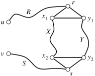
   Figure 7: A $u$–$v$-linked obstruction

   The following observation shows why $u$–$v$-linked obstructions are important:

   Lemma 20.

   Let $(G_{1},G_{2})$ be a separation of a graph $G$ with $V(G_{1}\cap G_{2})=\{u,v\}$. If $G_{1}$ contains a $u$–$v$-linked obstruction and $G_{2}$ has two induced $u$–$v$-paths of distinct parity, then $G$ contains $K_{4}$ as $t$-minor.

   Proof.

   Let $H$ be a $u$–$v$-linked obstruction in $G_{1}$ with paths $R,S,X,Y$.

   First, let $Y$ have even length. By assumption, there is an induced $u$–$v$-path in $G_{2}$ such that the length of the induced path $rRuPvSs$ is odd. Then, by $t$-contracting the vertices of degree $2$ of $H\cup P$ we arrive at $K_{4}$.

   Second, assume $Y$ to be an odd path, and choose $Q$ as an induced $u$–$v$-path in $G_{2}$ such that the induced path $rRuQvSs$ has even length. Again, $H\cup Q$ can be $t$-contracted to $K_{4}$. ∎

   Let us now prove that $u$–$v$-linked obstructions appear when induced $u$–$v$-paths of mixed parity are present:

   Lemma 21.

   Let $G$ be a claw- and $K_{4}$-free graph with $\Delta(G)\leq 4$. Let furthermore $G$ be $2$-connected, and let $(G_{1},G_{2})$ be a separation of $G$ with $V(G_{1}\cap G_{2})=\{u,v\}$. If there are two induced $u$–$v$-paths in $G_{1}$ of distinct parity, then $G_{1}$ contains a $u$–$v$-linked obstruction.

   Proof.

   Let $P$ and $Q$ be two induced $u$–$v$-paths, where $P$ has even length and $Q$ odd length. In particular, $uv\notin E(G)$. We, furthermore, choose $P$ and $Q$ such that $|V(P)\cup V(Q)|$ is minimum among all such pairs of paths. Let $P=p_{1}\ldots p_{r}$ and $Q=q_{1}\ldots q_{s}$, where $u=p_{1}=q_{1}$ and $v=p_{r}=q_{s}$.

   Let us first observe:

   any $$z\in V(G_{1}-Q) q\in V(Q) q Q$$ that has a neighbour is also adjacent to one of the neighbours of in . (18)

   Otherwise, there is a claw since $q$ has three independent neighbours: $z$ and its two neighbours in $Q$ (if $q=u$ or $q=v$ pick a neighbour of $q$ in $G_{2}$ instead – such a neighbour exists as $G$ is assumed to be $2$-connected).

   We now assume that there is a vertex $x$ of $P$ that has at least three neighbours in $Q$. In particular, $x$ does not belong to $Q$.

   If $x$ has exactly three neighbours in $Q$ we deduce from (18) that they appear consecutively on $Q$, that is, the neighbours are $q_{i}q_{i+1}q_{i+2}$ for some $i$. In that case, $Q+x$ is a $u$–$v$-linked obstruction, where we choose $R=uQq_{i}$, $S=q_{i+2}Qv$, $X=\{x\}$ and $Y=\{q_{i+1}\}$.

   If $x$ has more than three neighbours in $Q$, then it has exactly four as $\Delta(G)\leq 4$. By (18), there is $i<j$ so that the neighbours are $q_{i},q_{i+1},q_{j},q_{j+1}$. Again, we find that $Q+x$ is a $u$–$v$-linked obstruction: Set $R=uQq_{i}$, $S=q_{j+1}Qv$, $X=\{x\}$ and $Y=q_{i+1}Qq_{j}$.

   By symmetry, we may thus assume that

   every vertex of $$Q P$$ has at most two neighbours in , and vice versa. (19)

   Choose $i$ minimum such that $p_{i}\neq q_{i}$. As $P,Q$ are induced paths, this implies that $p_{i}\notin V(Q)$, from which with (18) follows that $p_{i}$ and $q_{i}$ are adjacent. Since $P$ and $Q$ have the same endvertex, we may moreover choose a minimum $j\geq i$ so that $p_{j+1}\in V(Q)$.

   We claim that

   no vertex of the path $$p_{i+1}Pp_{j-1} Q$$ has a neighbour in . (20)

   In order to prove the claim, suppose by way of contradiction that there is a minimum $\ell\in\{i+1,\ldots,j-1\}$ so that $p_{\ell}$ has a neighbour $x$ in $Q$.

   Suppose that $p_{\ell-1}x^{\prime}\in E(G)$ for some neighbour $x^{\prime}\in V(Q)$ of $p_{\ell}$, which by the minimality of $\ell$ is only possible when $i+1=\ell$. Since $p_{i+1}$ is not a neighbour of $q_{i-1}=p_{i-1}$, it follows that $x^{\prime}\neq q_{i-1}$. Then $x^{\prime}=q_{i}$, as $p_{i}$ cannot have three distinct neighbours $q_{i-1},q_{i},x^{\prime}$ in $Q$ by (19). But now $q_{i}$ has three neighbours in $P$, namely $p_{i-1},p_{i},p_{i+1}$, contradicting (19).

   In particular, with $x$ in the role of $x^{\prime}$, we obtain that $p_{\ell-1}x\notin E(G)$. The choice of $j$ together with $x\in V(Q)$ implies that $p_{\ell+1}\neq x$, as $\ell+1\leq j$. Thus, $x\notin V(P)$ and we deduce with (18) that $x$ is adjacent to $p_{\ell+1}$. Because also $p_{\ell}\notin V(Q)$ (by choice of $j$), we obtain from (18) that $p_{\ell}$ is adjacent to a neighbour $y$ of $x$ in $Q$. Again, $q_{i}\neq y$ as otherwise $q_{i}$ had the three neighbours $p_{i-1},p_{i},p_{\ell}$ in $P$, contradicting (19). We apply (18) again to see that $y$ is adjacent to either $p_{\ell-1}$ or to $p_{\ell+1}$. The former case, however, is impossible by the above observation that no neighbour $x^{\prime}\in V(Q)$ of $p_{\ell}$ is adjacent to $p_{\ell-1}$.

   Thus, $p_{\ell+1}y\in E(G)$, which means that $\{x,y,p_{l},p_{l+1}\}$ induces a $K_{4}$ in $G$, a contradiction. This proves (20).

   Let $p_{j+1}=q_{k}$, and observe that, as $p_{j}\notin V(Q)$ by minimality of $j$, it follows from (18) and (19) that $p_{j}$ is adjacent to $q_{k-1}$ or to $q_{k+1}$, but not to both.

   We first consider the case that $p_{j}q_{k-1}\in E(G)$. Suppose that the lengths of the paths $p_{i}Pp_{j}$ and $q_{i}Qq_{k-1}$ have the same parity. Then, we may replace in $Q$ the subpath $q_{i}Qq_{k-1}$ by $p_{i}Pp_{j}$. The obtained $u$–$v$-path $Q^{\prime}:=uQq_{i-1}Pp_{j}q_{k}Qv$ then has odd length, exactly as $Q$. Moreover, $Q^{\prime}$ is induced by (20). Since $|V(P)\cup V(Q^{\prime})|<|V(P)\cup V(Q)|$ we obtain a contradiction to the choice of $P$ and $Q$. Therefore, $p_{i}Pp_{j}$ and $q_{i}Qq_{k-1}$ have different parities. But then the subgraph induced by $Q\cup p_{i}Pp_{j}$ is a $u$–$v$-linked obstruction: We let $R=uQq_{i-1}$, $S=q_{k}Qv$, and for $X$ we choose the path among $p_{i}Pp_{j}$ and $q_{i}Qq_{k-1}$ of even length, and for $Y$ the odd one.

   If $p_{j}$ is adjacent to $p_{k+1}$ (and then not to $p_{k-1}$), we argue in a similar way in order to see that $p_{i}Pp_{j}$ and $q_{i}Qq_{k}$ have different parities. Then, we may choose $R=uQq_{i-1}$, $S=q_{k+1}Qv$, and $X,Y$ as $p_{i}Pp_{j}$ and $q_{i}Qq_{k}$, depending on the parity. ∎

   We can now prove our main lemma.

   Proof of Lemma 16.

   If the edge $uv$ is present in $G$, then every induced $u$–$v$-path in $G_{1}$ or in $G_{2}$ is odd (as the edge is the only induced path). Thus, we are in case (1(f)iv), which reduces to Lemma 14. Therefore, we may assume from now on that $uv\notin E(G)$.

   For (6(f)i), note that we may assume $G$ to be $K_{4}$-free, since $K_{4}$ is not $t$-perfect. Thus, Lemma 21 implies that $G_{1}$ contains a $u$–$v$-linked obstruction, which means we find $K_{4}$ as a $t$-minor in $G$, by Lemma 20. Thus $G$ is not $t$-perfect.

   For the forward direction of (1(f)i)–(1(f)iv), observe that the parity conditions guarantee that the respective $\tilde{G}_{1},\tilde{G}_{2}$ are $t$-minors of $G$. Thus, $t$-perfection of $G$ also implies their $t$-perfection.

   For the back direction of (1(f)i)–(1(f)iv), we assume $G$ to be $t$-imperfect. Note that $G\notin\{C_{7}^{2},C_{10}^{2}\}$ as both of the latter graphs are $3$-connected but $G$ is not. With Lemmas 18 and 19 we deduce that $G$ has a skewed prism $H$ consisting of two triangles $x_{1},x_{2},x_{3}$ and $y_{1},y_{2},y_{3}$ and of three linking paths $P_{i}=x_{i}\ldots y_{i}$ ($i=1,2,3$).

   Let us examine how $H$ can be positioned with respect to the separation $(G_{1},G_{2})$. There are three possibilities:

   1. $H\cap G_{1}$ is empty or $H\cap G_{2}$ is empty;

   2. $G$ contains $K_{4}$ as a subgraph; or

   3. $H\cap G_{1}$ is a subpath of one of $P_{1},P_{2},P_{3}$, or that is the case for $H\cap G_{2}$.

   In order to prove that (a)–(c) covers every case, we may by symmetry assume that $H\cap G_{2}$ contains the edge $x_{1}x_{2}$ of $H$. Now, we consider first the case when $H\cap G_{1}$ is non-empty but devoid of edges. In particular, that implies $H\subseteq G_{2}$. Let us assume that $u$ lies in $H\cap G_{1}$ (and possibly $v$, too). We observe that $u$ is adjacent to a vertex in $G_{1}$, as $G$ is $2$-connected. Thus, the absence of claws implies that the neighbours of $u$ in $G_{2}$ are pairwise adjacent. One of the three linking paths $P_{1},P_{2},P_{3}$ of $H$ contains $u$, $P_{1}$ say. We deduce that $P_{1}$ has to have length at most $1$, as otherwise the two neighbours of $u$ in $P_{1}\subseteq G_{2}$ is adjacent (if $u$ is an internal vertex) or one of the triangle vertices $x_{2},x_{3},y_{2},y_{3}$ is adjacent to an internal vertex of $P_{1}$ (if $u$ is an endvertex of $P_{1}$). Now, whether $P_{1}$ has length $0$ or $1$, in both cases $u$ has three distinct neighbours among $x_{1},x_{2},x_{3},y_{1},y_{2},y_{3}$. As those neighbours need to be pairwise adjacent, we have found $K_{4}$ as a subgraph of $G$.

   It remains to consider the case when $H\cap G_{1}$ is non-empty and contains an edge. Since any pair $x_{i},y_{j}$ is connected by three internally disjoint paths in $H$, we see that all of $x_{1},x_{2},x_{3},y_{1},y_{2},y_{3}$ lie in $G_{2}$. Therefore, any edge of $H$ in $G_{1}$ is an edge of one of the linking paths $P_{1},P_{2},P_{3}$, and clearly of only one of them. Thus, $H\cap G_{1}$ is a subpath of one of $P_{1},P_{2},P_{3}$. This proves that (a)–(c) exhaust all possibilities.

   We now apply (a)–(c) to the back direction of (1(f)i). If $H\cap G_{1}$ or $H\cap G_{2}$ is empty, then in particular $H$ is disjoint from $u,v$ and therefore, $H$ is still a skewed prism of either $G/_{u=v}$ or of $G_{2}+uv$. By Lemma 19, one of the two is then $t$-imperfect. If $G$ contains $K_{4}$ as a subgraph, then at most one of $u,v$ can lie in the $K_{4}$ as we assumed $uv\notin E(G)$. Consequently, $K_{4}$ is still a subgraph of one of $G/_{u=v}$ or $G_{2}+uv$.

   It remains to consider option (c). If $H\cap G_{1}$ is a subpath of one of $P_{1},P_{2},P_{3}$, then the subpath needs to be of odd length, as every induced $u$–$v$-path through $G_{2}$ is assumed to be of even length. Replacing the odd path through $G_{1}$ by the edge $uv$, we obtain a skewed prism of of $G_{2}+uv$, as desired. If, on the other hand, $H\cap G_{2}$ is a subpath of one of $P_{1},P_{2},P_{3}$ then this subpath has even length by assumption. That means restricting $H$ to $G_{1}$ while identifying $u$ with $v$ yields a skewed prism of $G_{1}/_{u=v}$, and we are done.

   Next, we treat the back direction of (1(f)ii). Observe that (a) and (b) imply that $H$ (or some $K_{4}$-subgraph) is completely contained in $G_{1}$ or in $G_{2}$, while (c) is impossible. Indeed, if $H\cap G_{1}$ (or $H\cap G_{2}$) was a subpath of one of $P_{1},P_{2},P_{3}$, then of necessarily even length, we would find an odd induced $u$–$v$-path in $H\cap G_{2}$ ($H\cap G_{1}$, respectively), contrary to assumption.

   The back directions of (1(f)iii) and (1(f)iv) are proved with similar arguments. ∎

   7 Discussion

   A key step for the recognition of claw-free $t$-perfect graphs is the insight of Lemmas 18 and 19 that the problem reduces to the detection of skewed prisms.

   Skewed prisms are induced subgraphs. As Fellows, Kratochvil, Middendorf and Pfeiffer [10] observed, searching for a certain substructure often becomes substantially harder if one requires the substructure to be induced: finding the largest matching can be done in polynomial time, but determining the size of the largest induced matching is NP-complete.

   In the same way, checking for a non-induced prism (and without any parity constraints on the paths) reduces to verifying whether between any two triangles there are three disjoint paths, which clearly can be done in polynomial time. Checking whether a given graph contains an induced prism, however, is NP-complete – this is a result of Maffray and Trotignon [20]. Interestingly, this changes when the input graph is claw-free. Golovach, Paulusma and van Leeuwen [13] describe a polynomial-time algorithm for the induced variant of the $k$-Disjoint Paths Problem in claw-free graphs. By again considering any pair of triangles in a claw-free graph, the algorithm may be used to detect prisms. Unfortunately, or rather fortunately for the purpose of this article, this is not enough to recognise $t$-perfection. For this, we need to detect skewed prisms. It is not clear whether the algorithm of Golovach, Paulusma and van Leeuwen can be extended to incorporate parity constraints.

   Kawarabayashi, Li and Reed [16] give a polynomial-time algorithm to detect subgraphs arising from $K_{4}$ by subdividing its edges to odd paths. In our terminology, these are (non-induced) subgraphs that can be $t$-contracted to $K_{4}$. Here the question arises whether one could develop and induced variant of their algorithm.

   Version

   Henning Bruhn <henning.bruhn@uni-ulm.de>
   Universität Ulm, Germany
   Oliver Schaudt <schaudto@uni-koeln.de>
   Institut für Informatik
   Universität zu Köln
   Weyertal 80
   Germany

References

- [1] M. Boulala and J.P. Uhry, Polytope des indépendants d’un graphe série-parallèle, Disc. Math. 27 (1979), 225–243.
- [2] H. Bruhn and M. Stein, -perfection is always strong for claw-free graphs, SIAM. J. Discrete Math. 24 (2010), 770–781.
- [3] , On claw-free t-perfect graphs, Math. Program. 133 (2012), 461–480.
- [4] M. Chudnovsky, G. Cornuéjols, X. Liu, P. Seymour, and K. Vušković, Recognizing berge graphs, Combinatorica 25 (2005), 143–187.
- [5] M. Chudnovsky, P. Seymour, N. Robertson, and R. Thomas, The strong perfect graph theorem, Ann. Math. 164 (2006), 51–229.
- [6] V. Chvátal, On certain polytopes associated with graphs, J. Combin. Theory (Series B) 18 (1975), 138–154.
- [7] T.H. Cormen, C.E. Leiserson, R.L. Rivest, and C. Stein, Introduction to algorithms (3rd edition), MIT press, 2009.
- [8] R. Diestel, Graph theory (4th edition), Springer-Verlag, 2010.
- [9] F. Eisenbrand, S. Funke, N. Garg, and J. Könemann, A combinatorial algorithm for computing a maximum independent set in a t-perfect graph, SODA, 2002, pp. 517–522.
- [10] M.R. Fellows, J. Kratochvil, M. Middendorf, and F. Pfeiffer, The complexity of induced minors and related problems, Algorithmica 13 (1995), 266–282.
- [11] J. Fonlupt and J.P. Uhry, Transformations which preserve perfectness and -perfectness of graphs, Ann. Disc. Math. 16 (1982), 83–95.
- [12] A.M.H. Gerards and F.B. Shepherd, The graphs with all subgraphs -perfect, SIAM J. Discrete Math. 11 (1998), 524–545.
- [13] P.A. Golovach, D. Paulusma, and E.J. van Leeuwen, Induced disjoint paths in claw-free graphs, arXiv:1202.4419v1.
- [14] T.C.T. Huynh, The linkage problem for group-labelled graphs, PhD thesis, University of Waterloo, 2009.
- [15] K. Kawarabayashi, Y. Kobayashi, and B. Reed, The disjoint paths problem in quadratic time, J. Combin. Theory (Series B) 102 (2012), 424–435.
- [16] K. Kawarabayashi, Z. Li, and B. Reed, Recognizing a totally odd -subdivision, parity 2-disjoint rooted paths and a parity cycle through specified elements, SODA, 2010, pp. 318–328.
- [17] K. Kawarabayashi, B. Reed, and P. Wollan, The graph minor algorithm with parity conditions, FOCS (2011), 27–36.
- [18] T. Király and J. Páp, A note on kernels in -perfect graphs, Tech. Report TR-2007-03, Egerváry Research Group, 2007.
- [19] , Kernels, stable matchings and Scarf’s Lemma, Tech. Report TR-2008-13, Egerváry Research Group, 2008.
- [20] F. Maffray and N. Trotignon, Algorithms for perfectly contractile graphs, SIAM J. Discrete Math 19 (2005), 553–574.
- [21] M.W. Padberg, Perfect zero-one matrices, Math. Programming 6 (1974), 180–196.
- [22] N.D. Roussopoulos, A algorithm for determining the graph from its line graph , Inf. Process. Lett. 2 (1973), 108–112.
- [23] N. Sbihi and J.P. Uhry, A class of h-perfect graphs, Disc. Math. 51 (1984), 191–205.
- [24] A. Schrijver, Strong -perfection of bad--free graphs, SIAM J. Discrete Math. 15 (2002), 403–415.
- [25] , Combinatorial optimization. Polyhedra and efficiency, Springer-Verlag, 2003.
- [26] F.B. Shepherd, Applying Lehman’s theorems to packing problems, Math. Prog. 71 (1995), 353–367.
- [27] T. Tholey, Solving the 2-disjoint paths problem in nearly linear time, Theory Comput. Syst. 39 (2006), 51–78.
- [28] P. van ’t Hof, M. Kamiński, and D. Paulusma, Finding induced paths of given parity in claw-free graphs, Algorithmica 62 (2012), 537–563.