Creation and protection of entanglement in systems out of thermal equilibrium

Abstract

We investigate the creation of entanglement between two quantum emitters interacting with a realistic common stationary electromagnetic field out of thermal equilibrium. In the case of two qubits we show that the absence of equilibrium allows the generation of steady entangled states, which is inaccessible at thermal equilibrium and is realized without any further external action on the two qubits. We first give a simple physical interpretation of the phenomenon in a specific case and then we report a detailed investigation on the dependence of the entanglement dynamics on the various physical parameters involved. Sub- and super-radiant effects are discussed, and qualitative differences in the dynamics concerning both creation and protection of entanglement according to the initial two-qubit state are pointed out.

1 Introduction

Quantum systems may present correlations of both quantum and classical nature. Entanglement captures quantum correlations due to the non separability of the system state [1, 2, 3]. The presence of these correlations is connected to the rise of non local effects in quantum theory [4] and has been recognized as a key resource in several fields of quantum technology, including quantum computing [5], quantum cryptography [6], quantum teleportation [7] and quantum metrology [8]. A main obstacle to the concrete exploitation of quantum features in the above applications is the detrimental effects of environmental noise [9]. The unavoidable coupling with degrees of freedom of the surrounding environment generally leads to a decay of quantum coherence properties [10], preventing the possible exploitation of quantum correlations present in the system.

A considerable effort has been done to understand the effects of environmental noise on the dynamics of correlations present in an open quantum system [11, 12, 13, 14, 15], and to contrast the natural fragility of quantum coherence properties [16, 17, 18]. Reservoir engineering methods have pointed out the possibility to change the perspective from reducing the coupling with the environment to modifying the environmental properties in order to manipulate the system of interest thanks to its proper dissipative dynamics [19, 20, 21]. Other approaches exploit the effect of measurements and feedback to drive the systems towards a target state [22, 23].

A possible way to create quantum correlations between two systems is to make them interact with a common environment [24], which can also cause a revival of entanglement [25]. In the case of two emitters in a common vacuum or thermal electromagnetic field, in absence of matter close to them, the mediated interaction plays a role over distances of the order of the common transition wavelength [26, 27]. It has been evidenced that the presence of plasmonic waveguides near the emitters can allow a mediated interaction over larger distances [28] whose effect on the entanglement dynamics has been discussed [29]. However, at thermal equilibrium the dynamical creation of entanglement eventually ceases at some time and the system thermalizes towards a thermal state which is a classical mixture. Steady entanglement can be instead generated by adding the action of an external driving laser [30].

The influence of several independent reservoirs at different temperatures, whose emission does not depend on their internal structure (material or geometry), has been considered in several contexts, including generation of entanglement in nonequilibrium steady states, both in the case of few spins [31, 32, 33] and of a chain of spins [34, 35, 36] and in the context of quantum thermal machines [37, 38].

However, in a realistic configuration the actual reflection and transmission properties of the bodies surrounding the quantum emitters should be taken into account, and may become particularly relevant if the emitters are placed close to the bodies (near-field effects). New possibilities emerging in such realistic systems out of thermal equilibrium have been recently pointed out in different contexts ranging from heat transfer [39, 40], to Casimir-Lifshits forces [41, 42, 43, 44, 45, 46]. There, radiation fields out of thermal equilibrium in configurations of quite general nature have been characterized in terms of the correlators of the total field depending on the scattering matrices of the bodies composing the total system [47, 48]. In the case of single emitters in such environments, new tools exploiting the absence of thermal equilibrium to manipulate the atomic dynamics realizing inversion of population and cooling of internal atomic temperature have been pointed out [49, 50]. Recently, the case of two quantum emitters has also been analyzed, pointing out a new remarkable mechanism to generate and protect entanglement in a steady way in systems out of thermal equilibrium [51].

In this paper, we report a detailed investigation of this phenomenon by studying the internal dynamics of a system composed by two quantum emitters (real atoms or artificial ones as quantum dots or superconducting qudits) placed in front of an arbitrary body embedded in a thermal radiation whose temperature is different from that of the body. The paper is organized as follows. In Sec. 2 we describe the physical model under investigation and we derive a master equation for the general case of two $N$-level emitters. In Sec. 3 we derive closed-form expressions for the functions governing the dynamics, in terms of the scattering matrices of the body and valid for arbitrary geometrical and material properties. In Sec. 4 we develop these expressions in the case when the body is a slab of finite thickness. From Sec. 5 on we specialize our analysis to the case of a two-qubit system, comparing cases in and out of thermal equilibrium. We point out the occurrence of peculiar phenomena emerging out of thermal equilibrium such as the generation of steady entanglement and a simple interpretation for this phenomenon is presented for a particularly interesting case. The general case of arbitrary values of the parameters is then discussed in Sec. 6. In Sec. 7 we draw our conclusions.

2 Model

We consider a system made of two quantum emitters $q=1,2$ interacting with an environment consisting of an electromagnetic field which is stationary and out of thermal equilibrium. This is generated by the field emitted by a body (M) at temperature $T_{\mathrm{M}}$ of arbitrary geometry and dielectric response and by the field emitted by the far surrounding walls (W) at temperature $T_{\mathrm{W}}$, which is eventually transmitted and reflected by the body itself (see figure 1).

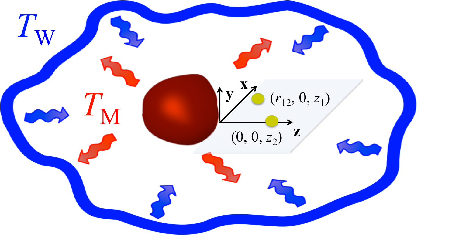
Figure 1: Physical configuration: two quantum emitters close to an arbitrary body whose temperature $T_{\mathrm{M}}$ is kept fixed and different from that of the surrounding walls $T_{\mathrm{W}}$. The two emitters are placed in $\mathbf{R}_{1}=(\mathbf{r}_{1},z_{1})$ and $\mathbf{R}_{2}=(\mathbf{r}_{2},z_{2})$, where $\mathbf{r}_{1}$ and $\mathbf{r}_{2}$ are vectors in the $xy$ plane. In the figure, we choose the $x$ axis along the direction $\mathbf{r}_{1}-\mathbf{r}_{2}$ and $x_{2}=0$, naming $r_{12}=|\mathbf{r}_{1}-\mathbf{r}_{2}|=x_{1}$ (this choice of the reference system is used in Sec. 4 in the specific case when the body is a slab).

$T_{\mathrm{M}}$ and $T_{\mathrm{W}}$ are kept fixed in time, realizing a stationary configuration for the electromagnetic field. The surrounding walls have an irregular shape and are distant enough from the body and the emitters so that their field can be treated at the emitters’ locations, in absence of the body, as a blackbody radiation independent from their composition. This is not true for the field emitted by the body M which cannot be treated as a blackbody since its radiation depend on its actual properties as its geometry and its dielectric function. The total Hamiltonian has the form

$$H=H_{S}+H_{E}+H_{I},$$ (1)

where $H_{S}$ and $H_{E}$ are the free Hamiltonians of the two emitters and of the environment. The interaction between the emitters and the field, in the multipolar coupling and in dipole approximation, is [52]

$$H_{I}=-\sum_{q}\mathbf{D}_{q}\cdot\mathbf{E}(\mathbf{R}_{q}),$$ (2)

where $\mathbf{D}_{q}$ is the electric-dipole operator of emitter $q$ and $\mathbf{E}(\mathbf{R}_{q})$ is the electric field at its position $\mathbf{R}_{q}$.

We first consider the general case in which each emitter has $N_{q}$ internal levels $|n\rangle_{q}$ where $n\in\{1,...,N_{q}\}$ of frequency $\omega_{n}^{q}$ (ordered by increasing energy). Given two arbitrary levels $n$ and $m$, their frequency difference is indicated by $\omega_{nm}^{q}=\omega_{n}^{q}-\omega_{m}^{q}$ and the transition matrix element of the dipole operator by $\mathbf{d}_{mn}^{q}={}_{q}\langle m|\mathbf{D}_{q}|n\rangle_{q}$. The free Hamiltonian of the two emitters is

$$H_{S}=\sum_{q=1}^{2}H_{q}=\sum_{q,\epsilon_{n}^{q}}\epsilon_{n}^{q}\Pi(\epsilon_{n}^{q}),$$ (3)

where $\Pi(\epsilon_{n}^{q})=|n\rangle_{q}{}_{q}\langle n|$ are the projectors associated to each eigenvalue $\epsilon_{n}^{q}=\hbar\omega_{n}^{q}$ (possibly degenerate) of $H_{q}$. The dipole operator of emitter $q$ in the interaction picture, $\mathbf{D}_{q}(t)=\exp(\frac{i}{\hbar}H_{S}t)\mathbf{D}_{q}\exp(-\frac{i}{\hbar}H_{S}t)$, results to be

$$\mathbf{D}_{q}(t)=\sum_{{}^{\,m,n}_{n>m}}\Bigl{(}\mathbf{d}_{mn}^{q}\ \sigma_{mn}^{q}e^{-i\omega_{nm}^{q}t}+\mathrm{h.c.}\Bigr{)},$$ (4)

where $\sigma_{mn}^{q}=|m\rangle_{q}{}_{q}\langle n|$ and $\omega_{nm}^{q}\geq 0$. By moving to the interaction picture, we obtain for $H_{I}$

$$H_{I}(t)=-\sum_{q}\mathbf{D}_{q}(t)\cdot\mathbf{E}(\mathbf{R}_{q},t),$$ (5)

where the time-dependent electric field is given by $\mathbf{E}(\mathbf{R}_{q},t)=\exp(\frac{i}{\hbar}H_{E}t)E(\mathbf{R}_{q})\exp(-\frac{i}{\hbar}H_{E}t)$. In the following each mode of the field is identified by the frequency $\omega$, the transverse wave vector $\mathbf{k}=(k_{x},k_{y})$, the polarization index $p$ (taking the values $p=1,2$ corresponding to transverse-electric (TE), and transverse-magnetic (TM) polarizations respectively), and the direction or propagation $\phi=\pm 1$ (shorthand notation $\phi=\pm$) along the $z$ axis [see figure 1]. In this approach, the total wavevector takes the form $\mathbf{K}^{\phi}=(\mathbf{k},\phi k_{z})$, where the $z$ component of the wavevector $k_{z}$ is a dependent variable given by $k_{z}=\sqrt{\frac{\omega^{2}}{c^{2}}-k^{2}}$, where $k=|\mathbf{k}|$. The explicit expression of the field at an arbitrary point $\mathbf{R}$ is

$$\mathbf{E}(\mathbf{R},t)=2\mathrm{Re}\Biggl{[}\int_{0}^{+\infty}\frac{d\omega}{2\pi}e^{-i\omega t}\mathbf{E}(\mathbf{R},\omega)\Biggr{]},$$ (6)

where a single-frequency component reads

$$\mathbf{E}(\mathbf{R},\omega)=\sum_{\phi,p}\int\frac{d^{2}\mathbf{k}}{(2\pi)^{2}}e^{i\mathbf{K}^{\phi}\cdot\mathbf{R}}\hat{\mbox{\boldmath$\epsilon$}}^{\phi}_{p}(\mathbf{k},\omega)E^{\phi}_{p}(\mathbf{k},\omega),$$ (7)

where $E^{\phi}_{p}(\mathbf{k},\omega)$ is the field amplitude operator associated to the mode $(\omega,\mathbf{k},p,\phi)$. For the TE and TM polarization vectors appearing in (7) we adopt the following standard definitions

$$\eqalign{\hat{\mbox{\boldmath$\epsilon$}}^{\phi}_{\mathrm{TE}}(\mathbf{k},\omega)&=\hat{\mathbf{z}}\times\hat{\mathbf{k}}=\frac{1}{k}(-k_{y}\hat{\mathbf{x}}+k_{x}\hat{\mathbf{y}}),\\ \hat{\mbox{\boldmath$\epsilon$}}^{\phi}_{\mathrm{TM}}(\mathbf{k},\omega)&=\frac{c}{\omega}\hat{\mbox{\boldmath$\epsilon$}}^{\phi}_{\mathrm{TE}}(\mathbf{k},\omega)\times\mathbf{K}^{\phi}=\frac{c}{\omega}(-k\hat{\mathbf{z}}+\phi k_{z}\hat{\mathbf{k}}),}$$ (8)

where $\hat{\mathbf{x}}$, $\hat{\mathbf{y}}$ and $\hat{\mathbf{z}}$ are the unit vectors along the three axes and $\hat{\mathbf{k}}=\mathbf{k}/k$.

2.1 Master equation

The starting point to study the dynamics of the two emitters is, in the interaction picture, the von Neumann equation for the total density matrix $\rho_{\mathrm{tot}}(t)$:

$$\frac{d}{dt}\rho_{\mathrm{tot}}(t)=-\frac{i}{\hbar}[H_{I}(t),\rho_{\mathrm{tot}}(t)].$$ (9)

The reduced density matrix of the two emitters is given by $\rho=\mathrm{Tr}_{E}[\rho_{\mathrm{tot}}]$, where $\mathrm{Tr}_{E}$ denotes the trace over the degrees of freedom of the environment. To derive a master equation for $\rho$ we follow the procedure described in [9] for the case of one emitter by extending it to our system made of two emitters. We name $\omega_{q}$ an arbitrary transition frequency of emitter $q$ (positive and negative). In general, several transitions can be characterized by the same frequency $\omega_{q}$ both because of degeneracy and/or the occurrence of equidistant levels. We rewrite each cartesian component of the dipole operator, $[\mathbf{D}_{q}]_{i}$ ($i=\{x,y,z\}$), as

$$[\mathbf{D}_{q}]_{i}=\sum_{\omega_{q}}\sum_{{}^{\>\>\>\>\{\epsilon^{q}_{n},\epsilon_{m}^{q}\}}_{\epsilon^{q}_{n}-\epsilon_{m}^{q}=\hbar\omega_{q}}}\Pi(\epsilon_{m}^{q})[\mathbf{D}_{q}]_{i}\Pi(\epsilon^{q}_{n})=\sum_{\omega_{q}}A^{q}_{i}(\omega_{q}),$$ (10)

where $A^{q}_{i}(\omega_{q})$ and $A^{q\,{\dagger}}_{i}(\omega_{q})$ turn out to be eigenoperators of $H_{q}$ with frequencies $-\omega_{q}$ and $+\omega_{q}$, respectively, i.e. $[H_{q},A_{i}^{q}(\omega_{q})]=-\omega_{q}A_{i}^{q}(\omega_{q})$ and $[H_{q},A_{i}^{q\,{\dagger}}(\omega_{q})]=+\omega_{q}A_{i}^{q\,{\dagger}}(\omega_{q})$. It also holds $A_{i}^{q\,{\dagger}}(\omega_{q})=A_{i}^{q}(-\omega_{q})$ and $\exp(\frac{i}{\hbar}H_{S}t)A^{q}_{i}(\omega_{q})\exp(-\frac{i}{\hbar}H_{S}t)=e^{-i\omega_{q}t}A^{q}_{i}(\omega_{q})$. In the central term of (10), the first sum is over all the frequencies $\omega_{q}$ while the second is over all the couples of energy eigenvalues $\epsilon^{q}_{n}$ and $\epsilon_{m}^{q}$ of $H_{q}$ such that $\epsilon^{q}_{n}-\epsilon_{m}^{q}=\hbar\omega_{q}$. Following [9], it is useful to rewrite $H_{I}(t)$ of (5) in terms of the eigenoperators $A^{q}_{i}(\omega_{q})$ as

$$H_{I}(t)=-\sum_{q}\sum_{i,\omega_{q}}e^{-i\omega_{q}t}A^{q}_{i}(\omega_{q})E_{i}(\mathbf{R}_{q},t).$$ (11)

From (10) it follows that the vector $\mathbf{A}^{q}(\omega_{q})=\{A^{q}_{x}(\omega_{q}),A^{q}_{y}(\omega_{q}),A^{q}_{z}(\omega_{q})\}$ is given by

$$\mathbf{A}^{q}(\omega_{q})=\sum_{{}^{\>\>\>\{m,n\}}_{\omega_{nm}^{q}=\omega_{q}}}\mathbf{d}_{mn}^{q}\sigma_{mn}^{q}=\mathbf{A}^{q\,{\dagger}}(-\omega_{q}),$$ (12)

where the sum is over all the couples $n$ and $m$ such that $\omega_{nm}^{q}=\omega_{q}$. By applying to the case of two emitters the standard procedure for the microscopic derivation of a master equation reported in [9], under Born, Markovian and rotating-wave approximations , one can obtain (using also the condition $\langle E_{i}(\mathbf{R},t)\rangle=0$) in the Schrödinger representation:

$$\eqalign{&\frac{d}{dt}\rho=-\frac{i}{\hbar}[H_{S},\rho]-i\sum_{q,q^{\prime},\omega}\sum_{i,i^{\prime}}\Big{\{}s_{ii^{\prime}}^{qq^{\prime}}(\omega)[A^{q\,{\dagger}}_{i}(\omega)A_{i^{\prime}}^{q^{\prime}}(\omega),\rho]\\ &\,+\gamma_{ii^{\prime}}^{qq^{\prime}}(\omega)\Big{(}A^{q^{\prime}}_{i^{\prime}}(\omega)\rho A^{q\,{\dagger}}_{i}(\omega)-\frac{1}{2}\{A^{q\,{\dagger}}_{i}(\omega)A^{q^{\prime}}_{i^{\prime}}(\omega),\rho\}\Big{)}\Big{\}},}$$ (13)

where $\omega\gtreqless 0$, being terms with positive or negative $\omega$ associated, respectively, to downward and upward transitions. In the above equation, for $q\neq q^{\prime}$ the sum $\sum_{q,q^{\prime},\omega}$ is over all common frequencies $\omega_{q}=\omega_{q^{\prime}}=\omega$ (this condition derives from the rotating wave approximation) while for $q=q^{\prime}$ it is over all transition frequencies of each emitter, and $\gamma_{ii^{\prime}}^{qq^{\prime}}(\omega)$, and $s_{ii^{\prime}}^{qq^{\prime}}(\omega)$ are defined by

$$\eqalign{\gamma_{ii^{\prime}}^{qq^{\prime}}(\omega)&=\Xi_{ii^{\prime}}^{qq^{\prime}}(\omega)+\Xi_{i^{\prime}i}^{q^{\prime}q\,*}(\omega),\quad s_{ii^{\prime}}^{qq^{\prime}}(\omega)=\frac{\Xi_{ii^{\prime}}^{qq^{\prime}}(\omega)-\Xi_{i^{\prime}i}^{q^{\prime}q\,*}(\omega)}{2i},\\ \Xi_{ii^{\prime}}^{qq^{\prime}}(\omega)&=\frac{1}{\hbar^{2}}\int_{0}^{\infty}\!\!ds\,e^{i\omega s}\langle E_{i}(\mathbf{R}_{q},t)E_{i^{\prime}}(\mathbf{R}_{q^{\prime}},t-s)\rangle,}$$ (14)

where the field correlation functions enter in the function $\Xi_{ii^{\prime}}^{qq^{\prime}}(\omega)$. It follows that $\Xi_{ii^{\prime}}^{qq^{\prime}}(\omega)=\frac{1}{2}\gamma_{ii^{\prime}}^{qq^{\prime}}(\omega)+is_{ii^{\prime}}^{qq^{\prime}}(\omega)$, $[\gamma_{ii^{\prime}}^{qq^{\prime}}(\omega)]^{*}=\gamma_{i^{\prime}i}^{q^{\prime}q}(\omega)$ and $[s_{ii^{\prime}}^{qq^{\prime}}(\omega)]^{*}=s_{i^{\prime}i}^{q^{\prime}q}(\omega)$.

The initial state of the total system in (13) is assumed to be factorized, $\rho_{\mathrm{tot}}(0)=\rho(0)\rho_{E}$. In the case $\rho_{E}$ is a stationary state of the environment ($[H_{E},\rho_{E}]=0$) the correlation functions are homogenous in time, that is $\langle E_{i}(\mathbf{R}_{q},t)E_{i^{\prime}}(\mathbf{R}_{q^{\prime}},t-s)\rangle=\langle E_{i}(\mathbf{R}_{q},s)E_{i^{\prime}}(\mathbf{R}_{q^{\prime}},0)\rangle$, so that

$$\gamma_{ii^{\prime}}^{qq^{\prime}}(\omega)=\frac{1}{\hbar^{2}}\int_{-\infty}^{\infty}ds\,e^{i\omega s}\langle E_{i}(\mathbf{R}_{q},s)E_{i^{\prime}}(\mathbf{R}_{q^{\prime}},0)\rangle$$ (15)

does not depend on time. The functions defined in (14) appearing in the master equation (13) depend thus only on the field correlation functions $\langle E_{i}(\mathbf{R}_{q},s)E_{i^{\prime}}(\mathbf{R}_{q^{\prime}},0)\rangle$, whose computation out of thermal equilibrium will be the subject of Secs. 3 and 4.

We now explicitly write the master equation (13) in the case of absence of degenerate and equidistant levels in each emitter, when the definition of eigenoperators $\mathbf{A}^{q}(\omega_{q})$ (12) reduces to $\mathbf{A}^{q}(\omega_{q})=\mathbf{d}^{q}_{mn}\sigma_{mn}^{q}$ (to each $\omega_{q}$ corresponds only one couple of energy eigenvalues $\{\epsilon^{q}_{m},\epsilon_{n}^{q}\}$). To this purpose, we develop the sum over $\omega$ in (13), which for each $|\omega|$ runs over $\omega$ (downward transitions) and $-\omega$ (upward transitions), as $\sum_{\omega}f(\omega)=\sum_{\omega>0}f(\omega)+\sum_{\omega>0}f(-\omega)$. From now on $\omega$ indicates always a positive frequency and we drop “$>0$” in the sums over $\omega$. Introducing this new convention and using the explicit form for $A^{q}_{i}(\omega)$ (12), we can recast (13) as

$$\eqalign{&\frac{d}{dt}\rho=-\frac{i}{\hbar}[H_{S},\rho]-i\sum_{q,\omega}\Bigl{\{}S^{qq}(\omega)[\sigma_{nn}^{q},\rho]+S^{qq}(-\omega)[\sigma_{mm}^{q},\rho]\Bigr{\}}\\ &\,-i\sum_{q\neq q^{\prime},\omega}\Lambda^{qq^{\prime}}(\omega)[\sigma_{mn}^{q\,{\dagger}}\sigma_{m^{\prime}n^{\prime}}^{q^{\prime}},\rho]+\sum_{q,q^{\prime},\omega}\Bigl{\{}\Gamma^{qq^{\prime}}(\omega)\Big{(}\sigma^{q^{\prime}}_{m^{\prime}n^{\prime}}\rho\sigma_{mn}^{q\,{\dagger}}\\ &\,-\frac{1}{2}\{\sigma^{q\,{\dagger}}_{mn}\sigma^{q^{\prime}}_{m^{\prime}n^{\prime}},\rho\}\Big{)}+\Gamma^{qq^{\prime}}(-\omega)\Big{(}\sigma^{q^{\prime}{\dagger}}_{m^{\prime}n^{\prime}}\rho\sigma^{q}_{mn}-\frac{1}{2}\{\sigma^{q}_{mn}\sigma^{q^{\prime}\,{\dagger}}_{m^{\prime}n^{\prime}},\rho\}\Big{)}\Bigr{\}},}$$ (16)

where the sum $\sum_{q,q^{\prime},\omega}$ in the second line is relative to all transition frequencies of each emitter for $q=q^{\prime}$ and only to the common transition frequencies for $q\neq q^{\prime}$, $(m,n)$ and $(m^{\prime},n^{\prime})$ individuate respectively the transition of each emitter corresponding to the frequency $\omega$, and we have defined the functions

$$\eqalign{S^{qq}(\omega)&=\sum_{i,i^{\prime}}s_{ii^{\prime}}^{qq}(\omega)[\textbf{d}_{mn}^{q}]^{*}_{i}[\textbf{d}_{mn}^{q}]_{i^{\prime}},\quad S^{qq}(-\omega)=\sum_{i,i^{\prime}}s_{ii^{\prime}}^{qq}(-\omega)[\textbf{d}_{mn}^{q}]_{i}[\textbf{d}_{mn}^{q}]^{*}_{i^{\prime}},\\ \Lambda^{qq^{\prime}}(\omega)&=\sum_{i,i^{\prime}}[\mathbf{d}_{mn}^{q}]_{i}^{*}[\mathbf{d}_{m^{\prime}n^{\prime}}^{q^{\prime}}]_{i^{\prime}}\bigl{[}s_{ii^{\prime}}^{qq^{\prime}}(\omega)+s_{i^{\prime}i}^{q^{\prime}q}(-\omega)\bigr{]},\\ \Gamma^{qq^{\prime}}(\omega)&=\sum_{i,i^{\prime}}\gamma_{ii^{\prime}}^{qq^{\prime}}(\omega)[\textbf{d}_{mn}^{q}]^{*}_{i}[\textbf{d}_{m^{\prime}n^{\prime}}^{q^{\prime}}]_{i^{\prime}},\quad\Gamma^{qq^{\prime}}(-\omega)=\sum_{i,i^{\prime}}\gamma_{ii^{\prime}}^{qq^{\prime}}(-\omega)[\textbf{d}_{mn}^{q}]_{i}[\textbf{d}_{m^{\prime}n^{\prime}}^{q^{\prime}}]^{*}_{i^{\prime}}.}$$ (17)

We remark that it holds $[\Lambda^{qq^{\prime}}(\omega)]^{*}=\Lambda^{q^{\prime}q}(\omega)$ and $[\Gamma^{qq^{\prime}}(\omega)]^{*}=\Gamma^{q^{\prime}q}(\omega)$. In (16), function $\Lambda^{qq^{\prime}}(\omega)$ represents a coherent (dipole-dipole) interaction between the emitters mediated by the field while dissipative effects enter through the $\Gamma$ functions. In particular, $\Gamma^{qq^{\prime}}(\pm\omega)$ are individual ($q=q^{\prime}$) and common field-mediated collective ($q\neq q^{\prime}$) emitter transition rates, related to both quantum and thermal fluctuations of the electromagnetic field at the emitters’ position.

3 Emitters close to an arbitrary body

Here we derive the field correlation functions needed to compute the functions in (17) for non equilibrium configurations in the case of an arbitrary body and multilevel emitters. These functions will depend on the two temperatures $T_{\mathrm{M}}$ and $T_{\mathrm{W}}$ and on the material and geometrical properties of the body as well. We follow the derivation discussed in [48] in the more general case of two bodies and three temperatures and the derivation relative to a single quantum emitter in the presence of a single body and two temperatures [50]. Here we extend the latter derivation to the case of two quantum emitters. Some of the computations involved are reported in A.

The starting point is to decompose, on the right side of the body where the emitters are located, the amplitude operators of total field modes propagating in the two directions $z>0$ and $z<0$ in terms of the fields emitted by the surrounding walls (W) and by the body (M). For a given set $(\omega,\mathbf{k},p)$, we have for the two directions

$$E^{+}=E^{(\mathrm{M})+}+\mathcal{T}E^{\mathrm{(W)}+}+\mathcal{R}E^{\mathrm{\mathrm{(W)}}-},\quad E^{-}=E^{\mathrm{(W)}-},$$ (18)

where we made the dependence on $\omega$, $\mathbf{k}$ and $p$ implicit. The total field $E^{-}$ propagating toward the body (i.e. toward the left) is equal to the field emitted by the walls $E^{(\mathrm{W})-}$ coming from the left, while the total field $E^{+}$ propagating toward the right results from the field $E^{(\mathrm{M})+}$ directly produced by the body, the transmission through the body of the field $E^{(\mathrm{W})+}$ emitted by the walls coming from the left, and the reflection by the body of the field $E^{(\mathrm{W})-}$ coming from the right [see figure 2].

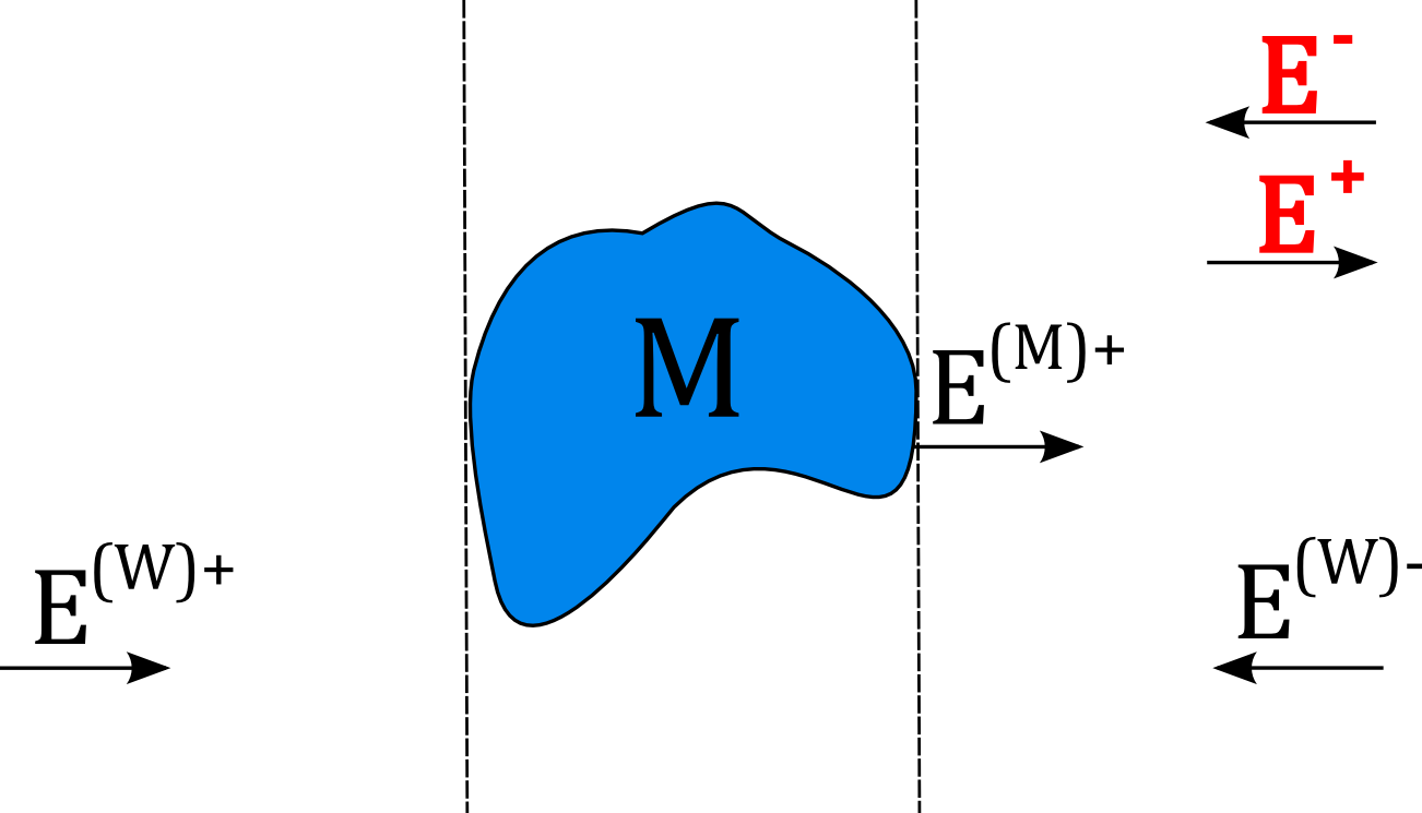
Figure 2: $E^{\pm}$ are the total field in the zone on the right of the body $\mathrm{M}$. $E^{(\mathrm{M})+}$ is the field emitted by the body towards the right, while $E^{(\mathrm{W})+}$ and $E^{(\mathrm{W})-}$ are the fields emitted by the surrounding walls (not shown in the picture) coming respectively from the left and from the right, eventually impinging on the body.

The operators $\mathcal{R}$ and $\mathcal{T}$ are the reflection and transmission scattering operators associated to the right side of the body, whose explicit definition can be found for example in [48]. They connect any outgoing (reflected or transmitted) mode of the field to the entire set of incoming modes. By using (18) one can write the total field correlators in terms of the correlators of the fields emitted by each source.

The source fields have been characterized as in [48] by assuming that for the body M and the walls W a local temperature which remains constant in time can be defined and that the emission process of the body is essentially not influenced by the presence of the external radiation impinging on the body itself. This assumption leads to the hypothesis that the part of the total field emitted by the body is the same as it would be if the body were at thermal equilibrium with the environment at its own temperature so that the correlators of the field emitted by each body can still be deduced using the fluctuation-dissipation theorem at its local temperature.

Under this assumption, the following symmetrized correlation functions [$\langle AB\rangle_{\mathrm{sym}}=(\langle AB\rangle+\langle BA\rangle)/2$] have been derived

$$\eqalign{&\langle E^{\mathrm{(M)}+}_{p}(\mathbf{k},\omega)E^{\mathrm{(M)}+{\dagger}}_{p^{\prime}}(\mathbf{k}^{\prime},\omega^{\prime})\rangle_{\mathrm{sym}}=\frac{\omega}{2\epsilon_{0}c^{2}}N(\omega,T_{\mathrm{M}})2\pi\delta(\omega-\omega^{\prime})\langle p,\mathbf{k}|\Bigl{(}\mathcal{P}_{-1}^{\mathrm{(pw)}}\\ &\,-\mathcal{R}\mathcal{P}_{-1}^{\mathrm{(pw)}}\mathcal{R}^{{\dagger}}+\mathcal{R}\mathcal{P}_{-1}^{\mathrm{(ew)}}-\mathcal{P}_{-1}^{\mathrm{(ew)}}\mathcal{R}^{{\dagger}}-\mathcal{T}\mathcal{P}_{-1}^{\mathrm{(pw)}}\mathcal{T}^{{\dagger}}\Bigr{)}|p^{\prime},\mathbf{k}^{\prime}\rangle,\\ &\langle E^{\mathrm{(W)}\phi}_{p}(\mathbf{k},\omega)E^{\mathrm{(W)}\phi^{\prime}{\dagger}}_{p^{\prime}}(\mathbf{k}^{\prime},\omega^{\prime})\rangle_{\mathrm{sym}}=\frac{\omega}{2\epsilon_{0}c^{2}}N(\omega,T_{\mathrm{W}})2\pi\delta(\omega-\omega^{\prime})\delta_{\phi,\phi^{\prime}}\langle p,\mathbf{k}|\mathcal{P}_{-1}^{\mathrm{(pw)}}|p^{\prime},\mathbf{k}^{\prime}\rangle,}$$ (19)

where we have introduced

$$\eqalign{&N(\omega,T)=\frac{\hbar\omega}{2}\coth\Bigl{(}\frac{\hbar\omega}{2k_{B}T}\Bigr{)}=\hbar\omega\Bigl{[}\frac{1}{2}+n(\omega,T)\Bigr{]},\quad n(\omega,T)=\Bigl{(}e^{\frac{\hbar\omega}{k_{B}T}}-1\Bigr{)}^{-1},\\ &\langle p,\mathbf{k}|\mathcal{P}_{n}^{\mathrm{(pw/ew)}}|p^{\prime},\mathbf{k}^{\prime}\rangle=k_{z}^{n}\langle p,\mathbf{k}|\Pi^{\mathrm{(pw/ew)}}|p^{\prime},\mathbf{k}^{\prime}\rangle.}$$ (20)

In the above equation $\Pi^{\mathrm{(pw)}}$ and $\Pi^{\mathrm{(ew)}}$ are the projectors on the propagative ($c\,k<\omega$, corresponding to a real $k_{z}$) and evanescent ($c\,k>\omega$, corresponding to a purely imaginary $k_{z}$) sectors respectively. By combining (18) and (19), in A a general expression for the total correlation functions in frequency space has been derived in (62). This expression can be used to compute the functions $\gamma_{ii^{\prime}}^{qq^{\prime}}(\omega),\gamma_{ii^{\prime}}^{qq^{\prime}}(-\omega)$ and $s_{ii^{\prime}}^{qq^{\prime}}(\omega)$ entering in (17), by exploiting their connection with the correlation functions between frequency components of the total field given in (63).

To move to the final expression of the functions in (17) we first rewrite the antinormally ordered correlation functions (62) as

$$\eqalign{\langle E_{i}&(\mathbf{R}_{q},\omega)E_{i^{\prime}}^{\dagger}(\mathbf{R}_{q^{\prime}},\omega)\rangle=\frac{\hbar\omega^{3}}{3\pi\epsilon_{0}c^{3}}\Big{\{}[1+n(\omega,T_{\mathrm{W}})]\\ &\times[\alpha_{\mathrm{W}}^{qq^{\prime}}(\omega)]_{ii^{\prime}}+[1+n(\omega,T_{\mathrm{M}})][\alpha_{\mathrm{M}}^{qq^{\prime}}(\omega)]_{ii^{\prime}}\Big{\}},}$$ (21)

from which the normally ordered correlation functions are obtained by replacing $\bigl{[}1+n(\omega,T_{i})\bigr{]}$ with $n(\omega,T_{i})$ and by taking the complex conjugate (this procedure derives from Kubo’s prescription as explained in A)

$$\eqalign{\langle E_{i}^{\dagger}&(\mathbf{R}_{q},\omega)E_{i^{\prime}}(\mathbf{R}_{q^{\prime}},\omega)\rangle=\frac{\hbar\omega^{3}}{3\pi\epsilon_{0}c^{3}}\Big{\{}n(\omega,T_{\mathrm{W}})\\ &\times[\alpha_{\mathrm{W}}^{qq^{\prime}}(\omega)]_{ii^{\prime}}^{*}+n(\omega,T_{\mathrm{M}})][\alpha_{\mathrm{M}}^{qq^{\prime}}(\omega)]_{ii^{\prime}}^{*}\Big{\}},}$$ (22)

and where we have introduced two $\alpha$ functions which do not depend on temperatures and on dipoles, and depend on the geometrical and material properties of the body through the operators $\mathcal{R}$ and $\mathcal{T}$:

$$\eqalign{[\alpha_{\mathrm{W}}^{qq^{\prime}}(\omega)]_{ii^{\prime}}&=\frac{3\pi c}{2\omega}\sum_{p,p^{\prime}}\int\frac{d^{2}\mathbf{k}}{(2\pi)^{2}}\int\frac{d^{2}\mathbf{k}^{\prime}}{(2\pi)^{2}}e^{i(\mathbf{k}\cdot\mathbf{r}_{q}-\mathbf{k}^{\prime}\cdot\mathbf{r}_{q^{\prime}})}\langle p,\mathbf{k}|\Bigl{\{}e^{i(k_{z}z_{q}-k_{z}^{{}^{\prime}*}z_{q^{\prime}})}\\ &\,\times[\hat{\mbox{\boldmath$\epsilon$}}_{p}^{+}(\mathbf{k},\omega)]_{i}[\hat{\mbox{\boldmath$\epsilon$}}_{p^{\prime}}^{+}(\mathbf{k}^{\prime},\omega)]_{i^{\prime}}^{*}\Bigl{(}\mathcal{T}\mathcal{P}_{-1}^{\mathrm{(pw)}}\mathcal{T}^{{\dagger}}+\mathcal{R}\mathcal{P}_{-1}^{\mathrm{(pw)}}\mathcal{R}^{{\dagger}}\Bigr{)}\\ &\,+e^{i(k_{z}z_{q}+k_{z}^{{}^{\prime}*}z_{q^{\prime}})}[\hat{\mbox{\boldmath$\epsilon$}}_{p}^{+}(\mathbf{k},\omega)]_{i}[\hat{\mbox{\boldmath$\epsilon$}}_{p^{\prime}}^{-}(\mathbf{k}^{\prime},\omega)]_{i^{\prime}}^{*}\mathcal{R}\mathcal{P}_{-1}^{\mathrm{(pw)}}\\ &\,+e^{-i(k_{z}z_{q}+k_{z}^{{}^{\prime}*}z_{q^{\prime}})}[\hat{\mbox{\boldmath$\epsilon$}}_{p}^{-}(\mathbf{k},\omega)]_{i}[\hat{\mbox{\boldmath$\epsilon$}}_{p^{\prime}}^{+}(\mathbf{k}^{\prime},\omega)]_{i^{\prime}}^{*}\mathcal{P}_{-1}^{\mathrm{(pw)}}\mathcal{R}^{{\dagger}}\\ &+e^{-i(k_{z}z_{q}-k_{z}^{{}^{\prime}*}z_{q^{\prime}})}[\hat{\mbox{\boldmath$\epsilon$}}_{p}^{-}(\mathbf{k},\omega)]_{i}[\hat{\mbox{\boldmath$\epsilon$}}_{p^{\prime}}^{-}(\mathbf{k}^{\prime},\omega)]_{i^{\prime}}^{*}\mathcal{P}_{-1}^{\mathrm{(pw)}}\Big{\}}|p^{\prime},\mathbf{k}^{\prime}\rangle,\\ [\alpha_{\mathrm{M}}^{qq^{\prime}}(\omega)]_{ii^{\prime}}&=\frac{3\pi c}{2\omega}\sum_{p,p^{\prime}}\int\frac{d^{2}\mathbf{k}}{(2\pi)^{2}}\int\frac{d^{2}\mathbf{k}^{\prime}}{(2\pi)^{2}}e^{i(\mathbf{k}\cdot\mathbf{r}_{q}-\mathbf{k}^{\prime}\cdot\mathbf{r}_{q^{\prime}})}\langle p,\mathbf{k}|\Bigl{\{}e^{i(k_{z}z_{q}-k_{z}^{{}^{\prime}*}z_{q^{\prime}})}\\ &\,\times[\hat{\mbox{\boldmath$\epsilon$}}_{p}^{+}(\mathbf{k},\omega)]_{i}[\hat{\mbox{\boldmath$\epsilon$}}_{p^{\prime}}^{+}(\mathbf{k}^{\prime},\omega)]_{i^{\prime}}^{*}\Bigl{[}\Bigl{(}\mathcal{P}_{-1}^{\mathrm{(pw)}}-\mathcal{R}\mathcal{P}_{-1}^{\mathrm{(pw)}}\mathcal{R}^{{\dagger}}+\mathcal{R}\mathcal{P}_{-1}^{\mathrm{(ew)}}\\ &\,-\mathcal{P}_{-1}^{\mathrm{(ew)}}\mathcal{R}^{{\dagger}}-\mathcal{T}\mathcal{P}_{-1}^{\mathrm{(pw)}}\mathcal{T}^{{\dagger}}\Bigr{)}\,\Big{\}}|p^{\prime},\mathbf{k}^{\prime}\rangle.}$$ (23)

Functions $[\alpha^{qq^{\prime}}_{\mathrm{W}}(\omega)]_{ii^{\prime}}$ and $[\alpha^{qq^{\prime}}_{\mathrm{M}}(\omega)]_{ii^{\prime}}$ are in general complex satisfying $\mathrm{Im}[\alpha^{qq^{\prime}}_{\mathrm{W}}(\omega)]_{ii^{\prime}}=-\mathrm{Im}[\alpha^{qq^{\prime}}_{\mathrm{M}}(\omega)]_{ii^{\prime}}$. The last property assures that the function $[\alpha^{qq^{\prime}}_{\mathrm{W}}(\omega)]_{ii^{\prime}}+[\alpha^{qq^{\prime}}_{\mathrm{M}}(\omega)]_{ii^{\prime}}$ is real as expected, being proportional to the imaginary part of the Green’s function [see (70)].

Now we can compute the transition rates in (17), using (63), (21) and (22),

$$\eqalign{\Gamma^{qq^{\prime}}(\omega)&=\sqrt{\Gamma_{0}^{q}(\omega)\Gamma_{0}^{q^{\prime}}(\omega)}\Big{\{}[1+n(\omega,T_{\mathrm{W}})]\alpha_{\mathrm{W}}^{qq^{\prime}}(\omega)+[1+n(\omega,T_{\mathrm{M}})]\alpha_{\mathrm{M}}^{qq^{\prime}}(\omega)\Big{\}}\\ \Gamma^{qq^{\prime}}(-\omega)&=\sqrt{\Gamma_{0}^{q}(\omega)\Gamma_{0}^{q^{\prime}}(\omega)}\Big{[}n(\omega,T_{\mathrm{W}})\alpha_{\mathrm{W}}^{qq^{\prime}}(\omega)^{*}+n(\omega,T_{\mathrm{M}})\alpha_{\mathrm{M}}^{qq^{\prime}}(\omega)^{*}\Big{]},}$$ (24)

where $\Gamma_{0}^{q}(\omega)=\frac{|\textbf{d}_{mn}^{q}|^{2}\omega^{3}}{3\hbar\pi\epsilon_{0}c^{3}}$ is the vacuum spontaneous-emission rate of transition $|n\rangle_{q}\to|m\rangle_{q}$ of emitter $q$ and we have introduced the new functions

$$\eqalign{\alpha_{\mathrm{W}}^{qq^{\prime}}(\omega)=\sum_{i,i^{\prime}}[\tilde{\textbf{d}}_{mn}^{q}]^{*}_{i}[\tilde{\textbf{d}}_{m^{\prime}n^{\prime}}^{q^{\prime}}]_{i^{\prime}}[\alpha_{\mathrm{W}}^{qq^{\prime}}(\omega)]_{ii^{\prime}}\quad\alpha_{\mathrm{M}}^{qq^{\prime}}(\omega)=\sum_{i,i^{\prime}}[\tilde{\textbf{d}}_{mn}^{q}]^{*}_{i}[\tilde{\textbf{d}}_{m^{\prime}n^{\prime}}^{q^{\prime}}]_{i^{\prime}}[\alpha_{\mathrm{M}}^{qq^{\prime}}(\omega)]_{ii^{\prime}},}$$ (25)

being $[\tilde{\textbf{d}}_{mn}^{q}]_{i}=[\textbf{d}_{mn}^{q}]_{i}/|\textbf{d}_{mn}^{q}|$. Differently from $[\alpha_{\mathrm{W(M)}}^{qq^{\prime}}(\omega)]_{ii^{\prime}}$, the functions $\alpha_{\mathrm{W(M)}}^{qq^{\prime}}(\omega)$ depend on the choice of emitters’ dipoles. In the case of two qubits, which will be treated in Secs. 5 and 6, there is only one transition for each emitter and above equations (24) and (25) hold with the notation $\textbf{d}_{mn}^{q}=\textbf{d}^{q}$.

With regards to the function $\Lambda^{qq^{\prime}}(\omega)$ we obtain, using (63), (21) and (22),

$$\eqalign{\Lambda^{qq^{\prime}}(\omega)=\frac{\sqrt{\Gamma_{0}^{q}(\omega)\Gamma_{0}^{q^{\prime}}(\omega)}}{\omega^{3}}\sum_{i,i^{\prime}}[\tilde{\mathbf{d}}_{mn}^{q}]_{i}^{*}[\tilde{\mathbf{d}}_{m^{\prime}n^{\prime}}^{q^{\prime}}]_{i^{\prime}}\mathcal{P}\int_{-\infty}^{+\infty}\frac{\omega^{\prime 3}d\omega^{\prime}}{2\pi}\frac{[\alpha_{\mathrm{W}}^{qq^{\prime}}(\omega^{\prime})]_{ii^{\prime}}+[\alpha_{\mathrm{M}}^{qq^{\prime}}(\omega^{\prime})]_{ii^{\prime}}}{\omega-\omega^{\prime}},}$$ (26)

where we used the properties $[\alpha_{\mathrm{W(M)}}^{qq^{\prime}}(\omega^{\prime})]_{ii^{\prime}}=[\alpha_{\mathrm{W(M)}}^{q^{\prime}q}(\omega^{\prime})]_{i^{\prime}i}^{*}$ and $[\alpha_{\mathrm{W(M)}}^{qq^{\prime}}(-\omega^{\prime})]_{ii^{\prime}}=[\alpha_{\mathrm{W(M)}}^{qq^{\prime}}(\omega^{\prime})]^{*}_{ii^{\prime}}$. It follows that $\Lambda^{qq^{\prime}}(\omega)$ does not depend on the presence or absence of thermal equilibrium, being independent on the temperatures. Using the relation between $\alpha$ functions of (23) and the Green’s function of the system in (70) derived in C, the integration over frequencies in (26) can be done by using the Kramers-Kronig relations connecting real and imaginary parts of the Green’s function:

$$\eqalign{\qquad\>\Lambda^{qq^{\prime}}(\omega)&=-\frac{1}{\hbar}\sum_{i,i^{\prime}}[\mathbf{d}_{mn}^{q}]_{i}^{*}[\mathbf{d}_{m^{\prime}n^{\prime}}^{q^{\prime}}]_{i^{\prime}}\mathcal{P}\int_{-\infty}^{+\infty}\frac{d\omega^{\prime}}{\pi}\frac{\mathrm{Im}\,G_{ii^{\prime}}(\mathbf{R}_{q},\mathbf{R}_{q^{\prime}},\omega^{\prime})}{\omega^{\prime}-\omega}\\ &=-\frac{1}{\hbar}\sum_{i,i^{\prime}}[\mathbf{d}_{mn}^{q}]_{i}^{*}[\mathbf{d}_{m^{\prime}n^{\prime}}^{q^{\prime}}]_{i^{\prime}}\mathrm{Re}\,G_{ii^{\prime}}(\mathbf{R}_{q},\mathbf{R}_{q^{\prime}},\omega).}$$ (27)

4 Emitters close to a slab

We now specialize the derivation of previous section to the case when the body is a slab of finite thickness $\delta$, defined by the two interfaces $z=0$ and $z=-\delta$ (see figure 3).

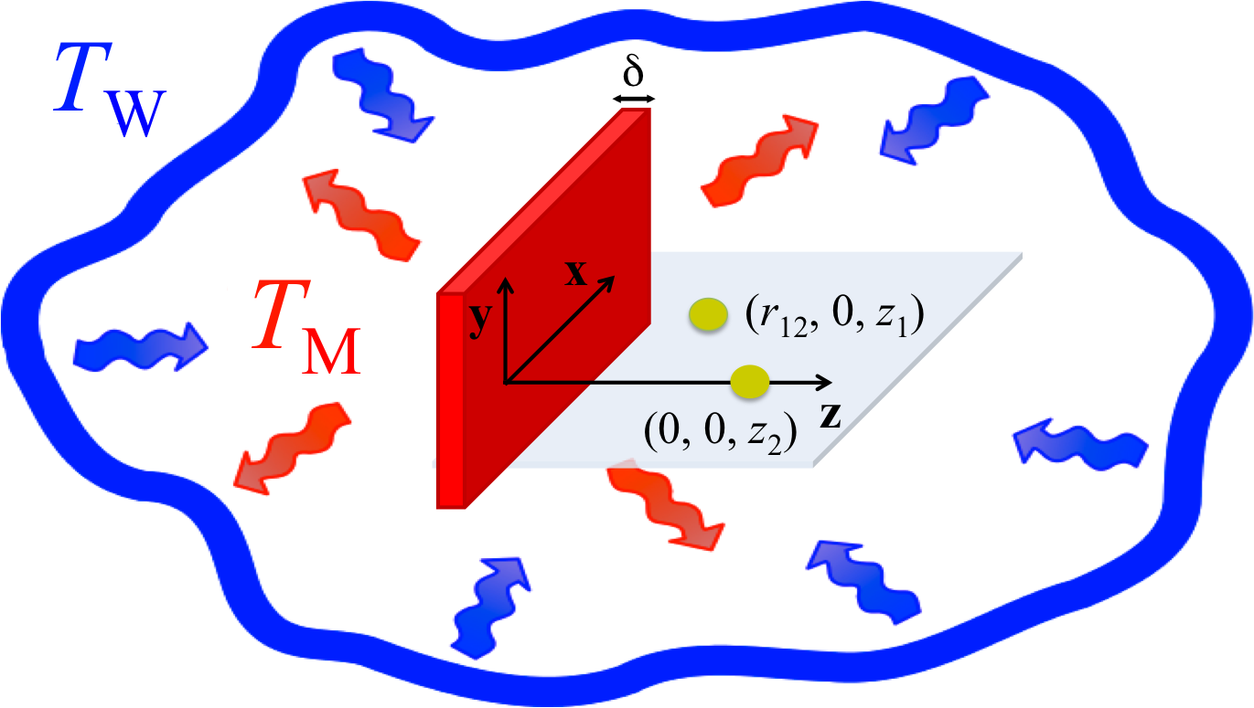
Figure 3: Two quantum emitters in front of a slab of thickness $\delta$ at a fixed temperature $T_{\mathrm{M}}$, surrounded by walls kept at a temperature $T_{\mathrm{W}}$.

In this simple case, explicit expressions for the transmission and reflection operators can be exploited [47, 48]. Because of the translational invariance of a planar slab with respect to the $xy$ plane, the slab reflection and transmission operators, $\mathcal{R}$ and $\mathcal{T}$, are diagonal and equal to

$$\eqalign{\langle p,\mathbf{k}|\mathcal{R}|p^{\prime},\mathbf{k}^{\prime}\rangle&=(2\pi)^{2}\delta(\mathbf{k}-\mathbf{k}^{\prime})\delta_{pp^{\prime}}\rho_{p}(\mathbf{k},\omega),\\ \langle p,\mathbf{k}|\mathcal{T}|p^{\prime},\mathbf{k}^{\prime}\rangle&=(2\pi)^{2}\delta(\mathbf{k}-\mathbf{k}^{\prime})\delta_{pp^{\prime}}\tau_{p}(\mathbf{k},\omega),}$$ (28)

where the Fresnel reflection and transmission coefficients modified by the finite thickness $\delta$ are given by (we recall that $p=1,2$ corresponding to TE and TM polarizations)

$$\eqalign{\rho_{p}(\mathbf{k},\omega)&=r_{p}(\mathbf{k},\omega)\frac{1-e^{2ik_{zm}\delta}}{1-r_{p}^{2}(\mathbf{k},\omega)e^{2ik_{zm}\delta}},\\ \tau_{p}(\mathbf{k},\omega)&=\frac{t_{p}(\mathbf{k},\omega)\bar{t}_{p}(\mathbf{k},\omega)e^{i(k_{zm}-k_{z})\delta}}{1-r_{p}^{2}(\mathbf{k},\omega)e^{2ik_{zm}\delta}}.\\ }$$ (29)

In the previous equations we have introduced the $z$ component of the $\mathbf{K}$ vector inside the medium,

$$k_{zm}=\sqrt{\varepsilon(\omega)\frac{\omega^{2}}{c^{2}}-\mathbf{k}^{2}},$$ (30)

$\varepsilon(\omega)$ being the dielectric permittivity of the slab, the ordinary vacuum-medium Fresnel reflection coefficients

$$r_{\mathrm{TE}}=\frac{k_{z}-k_{zm}}{k_{z}+k_{zm}},\qquad r_{\mathrm{TM}}=\frac{\varepsilon(\omega)k_{z}-k_{zm}}{\varepsilon(\omega)k_{z}+k_{zm}},$$ (31)

as well as both the vacuum-medium (noted with $t$) and medium-vacuum (noted with $\bar{t}$) transmission coefficients

$$\eqalign{t_{\mathrm{TE}}&=\frac{2k_{z}}{k_{z}+k_{zm}},\qquad\hskip 8.5359ptt_{\mathrm{TM}}=\frac{2\sqrt{\varepsilon(\omega)}k_{z}}{\varepsilon(\omega)k_{z}+k_{zm}},\\ \bar{t}_{\mathrm{TE}}&=\frac{2k_{zm}}{k_{z}+k_{zm}},\qquad\bar{t}_{\mathrm{TM}}=\frac{2\sqrt{\varepsilon(\omega)}k_{zm}}{\varepsilon(\omega)k_{z}+k_{zm}}.}$$ (32)

After replacing the matrix elements (28) in (23) we obtain for the $\alpha$ functions [we choose the $x$ axis along the vector $\mathbf{r}_{1}-\mathbf{r}_{2}$ whose coordinates in the plane $xy$ are then $(r_{12},0)$, being $r_{12}=|\mathbf{r}_{1}-\mathbf{r}_{2}|$],

$$\eqalign{[\alpha_{\mathrm{W}}^{qq^{\prime}}(\omega)]_{ii^{\prime}}=&\frac{3c}{8\pi\omega}\sum_{p}\Biggl{\{}\int_{0}^{\frac{\omega}{c}}\frac{dk\,k}{k_{z}}\Bigl{[}e^{ik_{z}(z_{q}-z_{q^{\prime}})}[N_{p}^{qq^{\prime}}(k,\omega)]^{++}_{ii^{\prime}}\bigl{(}|\rho_{p}(\mathbf{k},\omega)|^{2}+|\tau_{p}(\mathbf{k},\omega)|^{2}\bigr{)}\\ &+e^{ik_{z}(z_{q}+z_{q^{\prime}})}[N_{p}^{qq^{\prime}}(k,\omega)]^{+-}_{ii^{\prime}}\rho_{p}(\mathbf{k},\omega)+e^{-ik_{z}(z_{q}+z_{q^{\prime}})}[N_{p}^{qq^{\prime}}(k,\omega)]^{-+}_{ii^{\prime}}\rho_{p}(\mathbf{k},\omega)^{*}\\ &+e^{-ik_{z}(z_{q}-z_{q^{\prime}})}[N_{p}^{qq^{\prime}}(k,\omega)]^{--}_{ii^{\prime}}\Bigr{]}\Biggr{\}},\\ [\alpha_{\mathrm{M}}^{qq^{\prime}}(\omega)]_{ii^{\prime}}=&\frac{3c}{8\pi\omega}\sum_{p}\Biggl{\{}\int_{0}^{\frac{\omega}{c}}\frac{dk\,k}{k_{z}}e^{ik_{z}(z_{q}-z_{q^{\prime}})}[N_{p}^{qq^{\prime}}(k,\omega)]^{++}_{ii^{\prime}}\bigl{(}1-|\rho_{p}(\mathbf{k},\omega)|^{2}-|\tau_{p}(\mathbf{k},\omega)|^{2}\bigr{)}\\ &-i\int_{\frac{\omega}{c}}^{\infty}\frac{dk\,k}{\mathrm{Im}(k_{z})}e^{-\mathrm{Im}(k_{z})(z_{q}+z_{q^{\prime}})}[N_{p}^{qq^{\prime}}(k,\omega)]^{++}_{ii^{\prime}}\bigl{[}\rho_{p}(\mathbf{k},\omega)-\rho_{p}(\mathbf{k},\omega)^{*}\bigr{]}\Biggr{\}},}$$ (33)

where, using the fact that $\rho_{p}(\mathbf{k},\omega)$ and $\tau_{p}(\mathbf{k},\omega)$ are independent from $\theta$ (the angle formed by $\mathbf{k}$ and the $x$ axis in the plane $xy$), we have introduced the angular integrals

$$\eqalign{&[N_{p}^{qq^{\prime}}(k,\omega)]^{\phi\phi^{\prime}}_{ii^{\prime}}=\int_{0}^{2\pi}\frac{d\theta}{\pi}[\hat{\mbox{\boldmath$\epsilon$}}_{p}^{\phi}(\mathbf{k},\omega)]_{i}[\hat{\mbox{\boldmath$\epsilon$}}_{p}^{\phi^{\prime}}(\mathbf{k},\omega)]_{i^{\prime}}^{*}e^{ikr_{qq^{\prime}}\cos\theta},}$$ (34)

where $r_{21}=-r_{12}$. The matrix elements different from zero are, for $p=1$, $[N_{1}^{qq^{\prime}}]^{\phi\phi^{\prime}}_{11}=\frac{2}{kr_{qq^{\prime}}}J_{1}(kr_{qq^{\prime}})$, $[N_{1}^{qq^{\prime}}]^{\phi\phi^{\prime}}_{22}=\frac{2}{kr_{qq^{\prime}}}J_{1}(kr_{qq^{\prime}})-2J_{2}(kr_{qq^{\prime}})$, while for $p=2$ are

$$\eqalign{&[N_{2}^{qq^{\prime}}]^{\phi\phi^{\prime}}_{11}=\frac{2\phi\phi^{\prime}c^{2}|k_{z}^{2}|}{kr_{qq^{\prime}}\omega^{2}}\Big{[}J_{1}(kr_{qq^{\prime}})-kr_{qq^{\prime}}J_{2}(kr_{qq^{\prime}})\Big{]},\quad[N_{2}^{qq^{\prime}}]^{\phi\phi^{\prime}}_{13}=-i\phi\frac{2c^{2}kk_{z}}{\omega^{2}}J_{1}(kr_{qq^{\prime}}),\\ &[N_{2}^{qq^{\prime}}]^{\phi\phi^{\prime}}_{22}=\frac{2\phi\phi^{\prime}c^{2}|k_{z}^{2}|}{kr_{qq^{\prime}}\omega^{2}}J_{1}(kr_{qq^{\prime}}),\quad[N_{2}^{qq^{\prime}}]^{\phi\phi^{\prime}}_{31}=-i\phi^{\prime}\frac{2c^{2}kk_{z}^{*}}{\omega^{2}}J_{1}(kr_{qq^{\prime}}),\\ &[N_{2}^{qq^{\prime}}]^{\phi\phi^{\prime}}_{33}=\frac{2c^{2}k^{2}}{\omega^{2}}J_{0}(kr_{qq^{\prime}}),}$$ (35)

where $J_{n}(x)$ is the n-th order Bessel function of the first kind. For $x\to 0$, it is $J_{0}(x)\to 1$, $J_{1}(x)\to 0$, $J_{2}(x)\to 0$, and $J_{1}(x)/x\to 1/2$, so that $[N_{1(2)}^{qq^{\prime}}(k,\omega)]^{\phi\phi^{\prime}}_{ii^{\prime}}$ become diagonal and reduce to the vectors defined in (55) of [50] in the case of a single emitter.

To simplify the functions $[\alpha^{qq^{\prime}}_{\mathrm{W}}(\omega)]_{ii^{\prime}}$ and $[\alpha^{qq^{\prime}}_{\mathrm{M}}(\omega)]_{ii^{\prime}}$ in (33) we exploit the fact that the quantities $[N_{1}^{qq^{\prime}}(k,\omega)]^{\phi\phi^{\prime}}_{ii^{\prime}}$ do not depend on $\phi$ and $\phi^{\prime}$ and are real, and that in the propagative sector $[N_{2}^{qq^{\prime}}(k,\omega)]^{++}_{ii^{\prime}}=[N_{2}^{qq^{\prime}}(k,\omega)]^{--\,*}_{ii^{\prime}}$ and $[N_{2}^{qq^{\prime}}(k,\omega)]^{+-}_{ii^{\prime}}=[N_{2}^{qq^{\prime}}(k,\omega)]^{-+\,*}_{ii^{\prime}}$. Using the angular integrals (34), equation (33) can thus be rewritten as

$$\eqalign{[\alpha^{qq^{\prime}}_{\mathrm{W}}(\omega)]_{ii^{\prime}}&=\frac{[A^{qq^{\prime}}(\omega)]_{ii^{\prime}}^{*}+[B^{qq^{\prime}}(\omega)]_{ii^{\prime}}+2[C^{qq^{\prime}}(\omega)]_{ii^{\prime}}}{2},\\ _{ii^{\prime}}&=\frac{[A^{qq^{\prime}}(\omega)]_{ii^{\prime}}-[B^{qq^{\prime}}(\omega)]_{ii^{\prime}}+2[D^{qq^{\prime}}(\omega)]_{ii^{\prime}}}{2},}$$ (36)

where we have introduced the integral matrices

$$\eqalign{[A^{qq^{\prime}}(\omega)]_{ii^{\prime}}=&\frac{3c}{4\omega}\sum_{p}\int_{0}^{\frac{\omega}{c}}\frac{k\,dk}{k_{z}}e^{ik_{z}(z_{q}-z_{q^{\prime}})}[N_{p}^{qq^{\prime}}(k,\omega)]^{++}_{ii^{\prime}},\\ [B^{qq^{\prime}}(\omega)]_{ii^{\prime}}=&\frac{3c}{4\omega}\sum_{p}\int_{0}^{\frac{\omega}{c}}\frac{k\,dk}{k_{z}}e^{ik_{z}(z_{q}-z_{q^{\prime}})}[N_{p}^{qq^{\prime}}(k,\omega)]^{++}_{ii^{\prime}}\bigl{(}|\rho_{p}(k,\omega)|^{2}+|\tau_{p}(k,\omega)|^{2}\bigr{)},\\ [C^{qq^{\prime}}(\omega)]_{ii^{\prime}}=&\frac{3c}{4\omega}\sum_{p}\int_{0}^{\frac{\omega}{c}}\frac{k\,dk}{k_{z}}\mathrm{Re}\bigl{[}e^{ik_{z}(z_{q}+z_{q^{\prime}})}[N_{p}^{qq^{\prime}}(k,\omega)]^{+-}_{ii^{\prime}}\rho_{p}(k,\omega)\bigr{]},\\ [D^{qq^{\prime}}(\omega)]_{ii^{\prime}}=&\frac{3c}{4\omega}\sum_{p}\int_{\frac{\omega}{c}}^{+\infty}\!\!\!\!\frac{k\,dk}{\mathrm{Im}(k_{z})}e^{-\mathrm{Im}(k_{z})(z_{q}+z_{q^{\prime}})}[N_{p}^{qq^{\prime}}(k,\omega)]^{++}_{ii^{\prime}}\mathrm{Im}[\rho_{p}(k,\omega)].}$$ (37)

For $q=q^{\prime}$, $\alpha^{qq}_{\mathrm{W}}(\omega)$ and $\alpha^{qq}_{\mathrm{M}}(\omega)$ coincide with the functions defined in (56) of [50] in the case of a single emitter. For $q\neq q^{\prime}$, in the limit $\mathbf{R}_{q^{\prime}}\to\mathbf{R}_{q}$, $[\alpha^{qq^{\prime}}_{\mathrm{W}}(\omega)]_{ii^{\prime}}$ and $[\alpha^{qq^{\prime}}_{\mathrm{M}}(\omega)]_{ii^{\prime}}$ tend to their values in the case of a single emitter placed in $\mathbf{R}_{q}$. In the limit the distance between the two emitters goes to infinity, both $\alpha^{qq^{\prime}}_{\mathrm{W}}(\omega)$ and $\alpha^{qq^{\prime}}_{\mathrm{M}}(\omega)$ go to zero. In the limit of $|r_{qq^{\prime}}|\to\infty$, this is due to the fact that the functions $[N_{p}^{qq^{\prime}}(k,\omega)]^{\phi\phi^{\prime}}$ go to zero (for $|x|\to\infty$, it is $J_{0}(x)\to 0$, $J_{1}(x)\to 0$ and $J_{2}(x)\to 0$). In the limit $|z_{q}-z_{q^{\prime}}|\to\infty$, this is due to the presence of an oscillating functions whose frequency goes to infinity in the integrals $A(\omega)$, $B(\omega)$ and $C(\omega)$ (this can be seen explicitly by integrating by parts) and to the presence of the exponential function going to zero in the integral $D(\omega)$.

Concerning the function $\Lambda^{qq^{\prime}}(\omega)$, in order to develop its expression in (27) one has to compute the real part of the Green’s function in terms of the scattering operators $\mathcal{R}$ and $\mathcal{T}$. This is done in C where a free term $\Lambda_{0}^{qq^{\prime}}(\omega)$ [see (78)] remaining in absence of matter has been isolated from a reflected part $\Lambda_{R}^{qq^{\prime}}(\omega)$ [see (79)], $\Lambda^{qq^{\prime}}(\omega)=\Lambda_{0}^{qq^{\prime}}(\omega)+\Lambda_{R}^{qq^{\prime}}(\omega)$. Using the expressions for $\mathcal{R}$ and $\mathcal{T}$ in the case of a slab and the angular integrals in (34), one can derive, starting from (79):

$$\eqalign{&\mathrm{Re}\,G^{(R)}_{ii^{\prime}}(\mathbf{R}_{q},\mathbf{R}_{q^{\prime}},\omega)=\frac{i\omega^{2}}{4\epsilon_{0}c^{2}}\frac{1}{4\pi}\sum_{p}\Biggl{\{}\int_{0}^{\frac{\omega}{c}}\frac{k\,dk}{k_{z}}\Bigl{[}e^{ik_{z}(z_{q}+z_{q^{\prime}})}[N_{p}^{qq^{\prime}}(k,\omega)]^{+-}_{ii^{\prime}}\rho_{p}(\mathbf{k},\omega)\\ &\qquad-e^{-ik_{z}(z_{q}+z_{q^{\prime}})}[N_{p}^{qq^{\prime}}(k,\omega)]^{-+}_{ii^{\prime}}\rho_{p}(\mathbf{k},\omega)^{*}-i\int_{\frac{\omega}{c}}^{\infty}\frac{dk\,k}{\mathrm{Im}(k_{z})}e^{-\mathrm{Im}(k_{z})(z_{q}+z_{q^{\prime}})}\\ &\qquad\times[N_{p}^{qq^{\prime}}(k,\omega)]^{++}_{ii^{\prime}}\bigl{(}\rho_{p}(\mathbf{k},\omega)+\rho_{p}(\mathbf{k},\omega)^{*}\bigr{)}\Bigr{]}\Biggr{\}}.\\ }$$ (38)

Equation (27) can be thus cast under the form

$$\eqalign{\Lambda^{qq^{\prime}}(\omega)=&\Lambda_{0}^{qq^{\prime}}(\omega)+\sqrt{\Gamma_{0}^{q}(\omega)\Gamma_{0}^{q^{\prime}}(\omega)}\sum_{i,i^{\prime}}[\tilde{\textbf{d}}_{mn}^{q}]^{*}_{i}[\tilde{\textbf{d}}_{m^{\prime}n^{\prime}}^{q^{\prime}}]_{i^{\prime}}\bigr{(}[C_{2}^{qq^{\prime}}(\omega)]_{ii^{\prime}}-[D_{2}^{qq^{\prime}}(\omega)]_{ii^{\prime}}\bigr{)},}$$ (39)

where we have introduced the integral matrices

$$\eqalign{[C_{2}^{qq^{\prime}}(\omega)]_{ii^{\prime}}=&\frac{3c}{8\omega}\sum_{p}\int_{0}^{\frac{\omega}{c}}\frac{k\,dk}{k_{z}}\mathrm{Im}\bigl{[}e^{ik_{z}(z_{q}+z_{q^{\prime}})}[N_{p}^{qq^{\prime}}(k,\omega)]^{+-}_{ii^{\prime}}\rho_{p}(k,\omega)\bigr{]},\\ [D_{2}^{qq^{\prime}}(\omega)]_{ii^{\prime}}=&\frac{3c}{8\omega}\sum_{p}\int_{\frac{\omega}{c}}^{+\infty}\!\!\!\!\frac{k\,dk}{\mathrm{Im}(k_{z})}e^{-\mathrm{Im}(k_{z})(z_{q}+z_{q^{\prime}})}[N_{p}^{qq^{\prime}}(k,\omega)]^{++}_{ii^{\prime}}\mathrm{Re}\bigl{[}\rho_{p}(k,\omega)\bigr{]}.\\ }$$ (40)

We observe that the limit case when the body is absent is discussed in B, where known expressions for $\Gamma^{qq^{\prime}}(\omega)$ and $\Lambda^{qq^{\prime}}(\omega)$ are retrieved.

5 Two-qubit system

From now on we specialize our investigation to the case of two emitters (qubits) characterized by two internal levels $|1\rangle\equiv|g\rangle$ and $|2\rangle\equiv|e\rangle$ with the same transition frequency $\omega=\omega_{e}^{1}-\omega_{g}^{1}=\omega_{e}^{2}-\omega_{g}^{2}$. In this case, master equation (16) reduces to

$$\eqalign{\frac{d}{dt}\rho=&-\frac{i}{\hbar}[H_{S}+\delta_{S},\rho]-i\sum_{q\neq q^{\prime}}\Lambda^{qq^{\prime}}(\omega)[\sigma_{ge}^{q\,{\dagger}}\sigma_{ge}^{q^{\prime}},\rho]+\sum_{q,q^{\prime}}\Gamma^{qq^{\prime}}(\omega)\Big{(}\sigma^{q^{\prime}}_{ge}\rho\sigma_{ge}^{q\,{\dagger}}\\ &-\frac{1}{2}\{\sigma^{q\,{\dagger}}_{ge}\sigma^{q^{\prime}}_{ge},\rho\}\Big{)}+\sum_{q,q^{\prime}}\Gamma^{qq^{\prime}}(-\omega)\Big{(}\sigma^{q^{\prime}{\dagger}}_{ge}\rho\sigma^{q}_{ge}-\frac{1}{2}\{\sigma^{q}_{ge}\sigma^{q^{\prime}\,{\dagger}}_{ge},\rho\}\Big{)},}$$ (41)

where we used $[\sigma_{gg}^{q},\rho]=-[\sigma_{ee}^{q},\rho]$, so that

$$\delta_{S}=\sum_{q}\hbar\bigl{[}S^{qq}(\omega)-S^{qq}(-\omega)\bigr{]}\sigma_{ee}^{q},$$ (42)

and where the functions $S^{qq}(\pm\omega)$, $\Lambda^{qq^{\prime}}(\omega)$ and $\Gamma^{qq^{\prime}}(\pm\omega)$ are defined in (17) for the specific case $\{m,n\}=\{1,2\}$ (in the following we use the notation $\mathbf{d}_{12}^{q}=\mathbf{d}^{q}$).

We observe that master equation (41) can also describe the case in which the emitters’ frequencies are close enough (but not identical) so that rotating wave approximation used in the derivation of(13) still holds. This typically occurs when the frequency difference is much smaller than the average frequency [27]. The operator $\delta_{S}$ (42) represents a shift of energy levels, being the renormalized transition frequencies equal to $\tilde{\omega}_{e}^{1}-\omega_{g}^{1}=\omega+S^{11}(\omega)-S^{11}(-\omega)$ and $\tilde{\omega}_{e}^{2}-\omega_{g}^{2}=\omega+S^{22}(\omega)-S^{22}(-\omega)$. When these shifts are equal among them, that is $S^{11}(\omega)-S^{11}(-\omega)=S^{22}(\omega)-S^{22}(-\omega)$, as in the case of two identical qubits placed at the same distance from a slab, they do not play any relevant role in the dynamics. This is not the case in general, if the two shifts are not equal. However, in the cases treated in the following, we obtained numerical evidence that when they are not equal their influence is small and it will then be neglected.

To discuss the properties of (41), we will use two different bases, the decoupled basis $\{|1\rangle\equiv|gg\rangle,|2\rangle\equiv|eg\rangle,|3\rangle\equiv|ge\rangle,|4\rangle\equiv|ee\rangle\}$ and the coupled basis $\{|\mathrm{G}\rangle\equiv|1\rangle,|\mathrm{A}\rangle\equiv(|2\rangle-|3\rangle)/\sqrt{2},|\mathrm{S}\rangle\equiv(|2\rangle+|3\rangle)/\sqrt{2},|\mathrm{E}\rangle\equiv|4\rangle\}$, where we have introduced the collective antisymmetric $|\mathrm{A}\rangle$ and symmetric states $|\mathrm{S}\rangle$. The coupled basis is the one diagonalizing the effective Hamiltonian, $H_{S}+\sum_{q\neq q^{\prime}}\hbar\Lambda^{qq^{\prime}}(\omega)\sigma_{ge}^{q\,{\dagger}}\sigma_{ge}^{q^{\prime}}$, appearing in the first line of (41). In particular, the sign of $\Lambda^{12}(\omega)$ inverts the role of $|\mathrm{A}\rangle$ and $|\mathrm{S}\rangle$ in the eigenstates of the above effective Hamiltonian. The eigenvalues associated to $|\mathrm{G}\rangle$, $|\mathrm{A}\rangle$, $|\mathrm{S}\rangle$, $|\mathrm{E}\rangle$, are $\{0,$ $\hbar(\omega-|\Lambda^{12}(\omega)|),\hbar(\omega+|\Lambda^{12}(\omega)|),2\hbar\omega\}$, having set the energy of the ground state equal to zero.

5.1 X states

In the decoupled basis we can distinguish elements along the two main diagonals of the two-qubit density matrix from the remaining ones because they are not connected through master equation (41). We thus focus our attention on the class of X states, having non-zero elements only along the main diagonal and anti-diagonal of the density matrix (we use the notation $\rho_{ij}=\langle i|\rho|j\rangle$),

$$\rho_{X}=\left(\begin{array}[]{cccc}\rho_{11}&0&0&\rho_{14}\\ 0&\rho_{22}&\rho_{23}&0\\ 0&\rho_{23}^{*}&\rho_{33}&0\\ \rho_{14}^{*}&0&0&\rho_{44}\\ \end{array}\right).$$ (43)

Bell, Werner and Bell diagonal states belong to this class of states [56]. X-structure density matrices are found in a wide variety of physical situations and are also experimentally achievable [57]. For example, X states are encountered as eigenstates in all the systems with odd-even symmetry like in the Ising and the XY models [58]. Moreover, in many physical evolutions of open quantum systems an initial X structure is maintained in time [59], as it is in our case. Terms outside the two main diagonals initially populated, would be eventually washed off asymptotically. In the following, the two-qubit state will have always an X structure.

5.2 Concurrence

We shall quantify the entanglement in the two-qubit dynamics by evaluating the concurrence, $C(t)$ ($C=0$ for separable states, $C=1$ for maximally entangled states) [60]. For X states it takes the form [59]

$$\eqalign{C(t)&=2\,\mathrm{max}\{0,K_{1}(t),K_{2}(t)\},\\ K_{1}(t)&=|\rho_{23}(t)|-\sqrt{\rho_{11}(t)\rho_{44}(t)},\quad K_{2}(t)=|\rho_{14}(t)|-\sqrt{\rho_{22}(t)\rho_{33}(t)}.}$$ (44)

The master equation (41) always induces an exponential decay for $\rho_{14}(t)$, so that in the steady state only $K_{1}(t)$ could be responsible for having $C(\infty)>0$.

To discuss new phenomena emerging out of thermal equilibrium, it will be instructive to rewrite $K_{1}(t)$ in terms of the populations in the coupled basis (we use the notation $\rho_{\mathrm{IJ}}=\langle\mathrm{I}|\rho|\mathrm{J}\rangle$ and $\rho_{\mathrm{I}}=\langle\mathrm{I}|\rho|\mathrm{I}\rangle$):

$$\eqalign{K_{1}(t)=&\frac{1}{2}\sqrt{[\rho_{\mathrm{S}}(t)-\rho_{\mathrm{A}}(t)]^{2}+{|}\rho_{\mathrm{SA}}(t)-\rho_{\mathrm{AS}}(t){|}^{2}}-\sqrt{\rho_{\mathrm{G}}(t)\rho_{\mathrm{E}}(t)}.}$$ (45)

We will see that out of thermal equilibrium, it is always $\rho_{\mathrm{AS}}(\infty)=0$, but $\rho_{\mathrm{S}}(\infty)$ and $\rho_{\mathrm{A}}(\infty)$ can differ, so that $K_{1}(\infty)$ could be positive.

5.3 Thermal equilibrium

When $T_{\mathrm{W}}=T_{\mathrm{M}}\equiv T$, master equation (41) describes the thermalization towards the thermal equilibrium state, which is diagonal with the four steady populations given by

$$\left(\begin{array}[]{c}\rho_{11}(\infty)\\ \rho_{22}(\infty)\\ \rho_{33}(\infty)\\ \rho_{44}(\infty)\\ \end{array}\right)_{\!\!\!\mathrm{eq}}=\frac{1}{Z_{\mathrm{eq}}}\left(\begin{array}[]{c}[1+n(\omega,T)]^{2}\\ n(\omega,T)[1+n(\omega,T)]\\ n(\omega,T)[1+n(\omega,T)]\\ n(\omega,T)^{2}\\ \end{array}\right),$$ (46)

where $Z_{\mathrm{eq}}=[1+2n(\omega,T)]^{2}$. By moving to the coupled basis, the thermal state remains diagonal with $\rho_{\mathrm{S}}(\infty)=\rho_{\mathrm{A}}(\infty)=\rho_{22}(\infty)=\rho_{33}(\infty)$.

As a mathematical remark, we note that the thermal state is always reached asymptotically except if the identities $\Gamma^{11}(\pm\omega)=\Gamma^{22}(\pm\omega)=\Gamma^{12}(\pm\omega)=\Gamma^{21}(\pm\omega)\equiv\Gamma(\pm\omega)$ are strictly verified. In this peculiar case, both in and out of thermal equilibrium, the steady state depends upon the initial state and may be entangled. In particular, it is diagonal in the coupled basis with populations equal to

$$\left(\begin{array}[]{c}\rho_{\mathrm{G}}(\infty)\\ \rho_{\mathrm{A}}(\infty)\\ \rho_{\mathrm{S}}(\infty)\\ \rho_{\mathrm{E}}(\infty)\\ \end{array}\right)=\frac{1}{Z}\left(\begin{array}[]{c}\Gamma(\omega)^{2}[1-\rho_{\mathrm{A}}(0)]\\ \rho_{\mathrm{A}}(0)\\ \Gamma(-\omega)\Gamma(\omega)[1-\rho_{\mathrm{A}}(0)]\\ \Gamma(-\omega)^{2}[1-\rho_{\mathrm{A}}(0)]\end{array}\right),$$ (47)

where $Z=\Gamma(-\omega)^{2}+\Gamma(\omega)\Gamma(-\omega)+\Gamma(\omega)^{2}$. Apart from this case, at thermal equilibrium the steady state is always a thermal state, thus not entangled. We can see it by looking at the concurrence (44) which is zero being $\rho_{23}(\infty)=0$. This can also be seen in the coupled basis, where $\rho_{\mathrm{AS}}(\infty)=0$ and $\rho_{\mathrm{S}}(\infty)=\rho_{\mathrm{A}}(\infty)$, so that $K_{1}(\infty)$ (45) is negative.

5.4 Out of thermal equilibrium: an instructive case

When $T_{\mathrm{W}}\neq T_{\mathrm{M}}$, qualitative differences emerge in the dynamics and in the steady states. To highlight these new features, we first consider a simple case where a clear physical interpretation in terms of $|S\rangle$ and $|A\rangle$ is available. This is the case when $\Gamma^{11}(\pm\omega)=\Gamma^{22}(\pm\omega)\equiv\Gamma(\pm\omega)$ and $\Gamma^{12(21)}(\pm\omega)$ are real. These conditions are verified, for example, in the case of identical qubits, with $\mathbf{d}^{1}=\mathbf{d}^{2}\equiv\mathbf{d}$, placed in equivalent positions with respect to the body (in the case of a slab, $z_{1}=z_{2}$) and with $\mathbf{d}$ real and having components different from zero either only along the $z$ axis or only along the plane $xy$. In this case, master equation (41) gives in the coupled basis a set of rate equations for the populations, which are decoupled from the other density matrix elements:

$$\eqalign{\dot{\rho}_{\mathrm{G}}=&-(\Gamma_{\mathrm{A}}\,n_{\mathrm{A}}+\Gamma_{\mathrm{S}}\,n_{\mathrm{S}})\rho_{\mathrm{G}}+\Gamma_{\mathrm{A}}(1+n_{\mathrm{A}})\rho_{\mathrm{A}}+\Gamma_{\mathrm{S}}(1+n_{\mathrm{S}})\rho_{\mathrm{S}},\\ \dot{\rho}_{\mathrm{A}}=&-\Gamma_{\mathrm{A}}(1+2n_{\mathrm{A}})\rho_{\mathrm{A}}+\Gamma_{\mathrm{A}}\,n_{\mathrm{A}}\rho_{\mathrm{G}}+\Gamma_{\mathrm{A}}(1+n_{\mathrm{A}})\rho_{\mathrm{E}},\\ \dot{\rho}_{\mathrm{S}}=&-\Gamma_{\mathrm{S}}(1+2n_{\mathrm{S}})\rho_{\mathrm{S}}+\Gamma_{\mathrm{S}}\,n_{\mathrm{S}}\rho_{\mathrm{G}}+\Gamma_{\mathrm{S}}(1+n_{\mathrm{S}})\rho_{\mathrm{E}},\\ \dot{\rho}_{\mathrm{E}}=&-[\Gamma_{\mathrm{A}}{(1+n_{\mathrm{A}})}+\Gamma_{\mathrm{S}}{(1+n_{\mathrm{S}})}]\rho_{\mathrm{E}}+\Gamma_{\mathrm{A}}\,n_{\mathrm{A}}\rho_{\mathrm{A}}+\Gamma_{\mathrm{S}}\,n_{\mathrm{S}}\rho_{\mathrm{S}}.}$$ (48)

Here the coefficient $\Gamma_{0}(\omega)$ has been absorbed by the time variable in the derivative, which is now dimensionless, and we have used the relations

$$\eqalign{\Gamma(\omega)-\Gamma^{12}(\omega)=\Gamma_{0}(\omega)\Gamma_{\mathrm{A}}(1+n_{\mathrm{A}}),\quad\Gamma(\omega)+\Gamma^{12}(\omega)=\Gamma_{0}(\omega)\Gamma_{\mathrm{S}}(1+n_{\mathrm{S}}),\\ \Gamma(-\omega)-\Gamma^{12}(-\omega)=\Gamma_{0}(\omega)\Gamma_{\mathrm{A}}\,n_{\mathrm{A}},\quad\Gamma(-\omega)+\Gamma^{12}(-\omega)=\Gamma_{0}(\omega)\Gamma_{\mathrm{S}}\,n_{\mathrm{S}},}$$ (49)

with

$$\eqalign{\Gamma_{\mathrm{A}}=\alpha_{\mathrm{W}}(\omega)-\alpha^{12}_{\mathrm{W}}(\omega)+\alpha_{\mathrm{M}}(\omega)-\alpha^{12}_{\mathrm{M}}(\omega),\\ \Gamma_{\mathrm{S}}=\alpha_{\mathrm{W}}(\omega)+\alpha^{12}_{\mathrm{W}}(\omega)+\alpha_{\mathrm{M}}(\omega)+\alpha^{12}_{\mathrm{M}}(\omega),\\ n_{\mathrm{A}}=\frac{1}{\Gamma_{\mathrm{A}}}\Bigl{\{}\left[\alpha_{\mathrm{W}}(\omega)-\alpha^{12}_{\mathrm{W}}(\omega)\right]n(\omega,T_{\mathrm{W}})+\left[\alpha_{\mathrm{M}}(\omega)-\alpha^{12}_{\mathrm{M}}(\omega)\right]n(\omega,T_{\mathrm{M}})\Bigr{\}},\\ n_{\mathrm{S}}=\frac{1}{\Gamma_{\mathrm{S}}}\Bigl{\{}\left[\alpha_{\mathrm{W}}(\omega)+\alpha^{12}_{\mathrm{W}}(\omega)\right]n(\omega,T_{\mathrm{W}})+\left[\alpha_{\mathrm{M}}(\omega)+\alpha^{12}_{\mathrm{M}}(\omega)\right]n(\omega,T_{\mathrm{M}})\Bigr{\}},}$$ (50)

where $\alpha_{\mathrm{W(M)}}(\omega)\equiv\alpha^{11}_{\mathrm{W(M)}}(\omega)=\alpha^{22}_{\mathrm{W(M)}}(\omega)$. We remark that $\Lambda^{qq^{\prime}}(\omega)$ does not enter in the rate equations (48), which are schematically represented in figure 4. We observe that to each decay channel from $|\mathrm{E}\rangle$ to $|\mathrm{G}\rangle$ we can associate distinct effective temperatures $T_{\mathrm{S}}$ and $T_{\mathrm{A}}$ confined between $T_{\mathrm{W}}$ and $T_{\mathrm{M}}$ in correspondence to the effective number of photons $n_{\mathrm{S}}$ and $n_{\mathrm{A}}$, which have the property of being confined between $n(\omega,T_{\mathrm{W}})$ and $n(\omega,T_{\mathrm{M}})$ [50].

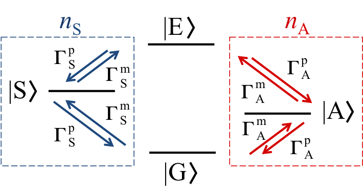
Figure 4: Representation of the rate equations (48). The transition rates in the two channels are $\Gamma^{\mathrm{p}}_{\mathrm{S}(\mathrm{A})}=\Gamma_{\mathrm{S}(\mathrm{A})}(1+n_{\mathrm{S}(\mathrm{A})})$ and $\Gamma^{\mathrm{m}}_{\mathrm{S}(\mathrm{A})}=\Gamma_{\mathrm{S}(\mathrm{A})}\,n_{\mathrm{S}(\mathrm{A})}.$

Concerning the coherences in the second diagonal:

$$\eqalign{\dot{\rho}_{\mathrm{A}\mathrm{S}}=&-\frac{1}{2}\left[\Gamma_{\mathrm{A}}(1+2n_{\mathrm{A}})+\Gamma_{\mathrm{S}}(1+2n_{\mathrm{S}})-4i\Lambda^{12}(\omega)\right]\rho_{\mathrm{A}\mathrm{S}},\\ \dot{\rho}_{\mathrm{G}\mathrm{E}}=&-\frac{1}{2}\left[\Gamma_{\mathrm{A}}(1+2n_{\mathrm{A}})+\Gamma_{\mathrm{S}}(1+2n_{\mathrm{S}})-4i{\omega}\right]\rho_{\mathrm{G}\mathrm{E}},\\ }$$ (51)

which give for each coherence an exponential decay modulating oscillations due , respectively, to $\Lambda^{12}(\omega)$ and $\omega$. The stationary solution of (48) is

$$\eqalign{&\left(\begin{array}[]{c}\rho_{\mathrm{G}}(\infty)\\ \\ \rho_{\mathrm{A}}(\infty)\\ \\ \rho_{\mathrm{S}}(\infty)\\ \\ \rho_{\mathrm{E}}(\infty)\\ \end{array}\right)_{\!\!\!\mathrm{neq}}=\frac{1}{Z_{\mathrm{neq}}}\left(\begin{array}[]{c}(1+n_{\mathrm{A}})^{2}(1+2n_{\mathrm{S}})\Gamma_{\mathrm{A}}+(1+2n_{\mathrm{A}})(1+n_{\mathrm{S}})^{2}\Gamma_{\mathrm{S}}\\ \\ n_{\mathrm{A}}(1+n_{\mathrm{A}})(1+2n_{\mathrm{S}})\Gamma_{\mathrm{A}}+[n_{\mathrm{A}}(1+2n_{\mathrm{S}})\\ +n_{\mathrm{S}}^{2}(1+2n_{\mathrm{A}})]\Gamma_{\mathrm{S}}\\ \\ n_{\mathrm{S}}(1+n_{\mathrm{S}})(1+2n_{\mathrm{A}})\Gamma_{\mathrm{S}}+[n_{\mathrm{S}}(1+2n_{\mathrm{A}})\\ +n_{\mathrm{A}}^{2}(1+2n_{\mathrm{S}})]\Gamma_{\mathrm{A}}\\ \\ n_{\mathrm{A}}^{2}(1+2n_{\mathrm{S}})\Gamma_{\mathrm{A}}+(1+2n_{\mathrm{A}})n_{\mathrm{S}}^{2}\Gamma_{\mathrm{S}}\end{array}\right),}$$ (52)

where $Z_{\mathrm{neq}}$ is the sum of the elements of the vector in the second line of the above equation. Out of equilibrium $\rho_{23}(\infty)_{\mathrm{neq}}$ is different from zero and is given by:

$$\eqalign{\rho_{23}(\infty)_{\mathrm{neq}}=\frac{(n_{\mathrm{S}}-n_{\mathrm{A}})(\Gamma_{\mathrm{S}}+\Gamma_{\mathrm{A}})}{2Z_{\mathrm{neq}}},}$$ (53)

where we see easily how it tends to zero at thermal equilibrium when $n_{\mathrm{S}}=n_{\mathrm{A}}$. Using (LABEL:ote_case) in (44) and (45), we obtain for the steady concurrence:

$$\eqalign{C(\infty)_{\mathrm{neq}}=&\frac{2}{Z_{\mathrm{neq}}}\Bigl{[}|n_{\mathrm{S}}-n_{\mathrm{A}}|(\Gamma_{\mathrm{S}}+\Gamma_{\mathrm{A}})/2\\ &\,-\sqrt{(1+n_{\mathrm{A}})^{2}(1+2n_{\mathrm{S}})\Gamma_{\mathrm{A}}+(1+2n_{\mathrm{A}})(1+n_{\mathrm{S}})^{2}\Gamma_{\mathrm{S}}}\\ &\,\times\sqrt{n_{\mathrm{A}}^{2}(1+2n_{\mathrm{S}})\Gamma_{\mathrm{A}}+(1+2n_{\mathrm{A}})n_{\mathrm{S}}^{2}\Gamma_{\mathrm{S}}}\;\Bigr{]}.}$$ (54)

Figure 5: $C=C(\infty)_{\mathrm{neq}}$ vs $n_{\mathrm{A}}$ for $n_{\mathrm{S}}=10^{-3}$ for different values of $\Gamma_{\mathrm{A}}/\Gamma_{\mathrm{S}}$ indicated in the legend.

Simplifying $\Gamma_{\mathrm{S}}$, $C(\infty)_{\mathrm{neq}}$ becomes function of the three dimensionless quantities $\Gamma_{\mathrm{A}}/\Gamma_{\mathrm{S}}$, $n_{\mathrm{S}}$ and $n_{\mathrm{A}}$. This dependence is discussed in figure 5, where $C=C(\infty)_{\mathrm{neq}}$ is depicted as a function of $n_{\mathrm{A}}$ for $n_{\mathrm{S}}=0.001$ and for several values of $\Gamma_{\mathrm{A}}/\Gamma_{\mathrm{S}}$, as indicated in the legend. We observe that by decreasing the value of $\Gamma_{\mathrm{A}}/\Gamma_{\mathrm{S}}$, higher values of $C$ are reachable at higher values of $n_{\mathrm{A}}$. The maximum value of $C$ is 1/3, which can be obtained in the limits $\Gamma_{\mathrm{A}}/\Gamma_{\mathrm{S}}\to 0,n_{\mathrm{S}}\to 0$ and $n_{\mathrm{A}}\to\infty$. In particular, the corresponding maximally entangled state, which is a statistical mixture of the ground and of the antisymmetric state with weights respectively equal to 2/3 and 1/3, has also been found in [36]. For smaller values of $n_{\mathrm{S}}$ the behavior remains almost identical, while by increasing its value, the values of $C$ decrease progressively. We remark that an identical behavior is found in the opposite case, i.e. when $\Gamma_{\mathrm{S}}/\Gamma_{\mathrm{A}}\to 0$, case in which the role of states $|\mathrm{S}\rangle$ and $|\mathrm{A}\rangle$ is inverted. This can be achieved by looking for values of the various parameters such that $\alpha^{12}_{\mathrm{M(W)}}(\omega)$ is negative and very close to $\alpha_{\mathrm{M(W)}}(\omega)$ in order make the ratio $\Gamma_{\mathrm{S}}/\Gamma_{\mathrm{A}}$ very small.

Figure 5 describes the generation of steady entangled states emerging only in the absence of thermal equilibrium. Two main conditions must be fulfilled, the first being to have small values for $\Gamma_{\mathrm{A}}/\Gamma_{\mathrm{S}}$ and the second to realize (quite) different effective temperatures for the two decay channels, which can be achieved only in absence of thermal equilibrium.

6 Numerical investigation

Here we report the numerical investigation concerning the case treated in Sec. 4 when the body close to the emitters is a slab of finite thickness $\delta$. According to (13), a relevant parameter involved in our investigation concerning the role of the body is the value of the dielectric permittivity at the common transition frequency of the two qubits. As material we choose the silicon carbide (SiC) whose dielectric permittivity $\varepsilon(\omega)$ is described using a Drude-Lorentz model [54]

$$\varepsilon(\omega)=\varepsilon_{\infty}\frac{\omega^{2}-\omega_{l}^{2}+i\Gamma\omega}{\omega^{2}-\omega_{r}^{2}+i\Gamma\omega},$$ (55)

characterized by a resonance at $\omega_{r}=1.495\times 10^{14}\,\mathrm{rad}\,\mathrm{s}^{-1}$ and where $\varepsilon_{\infty}=6.7$, $\omega_{l}=1.827\times 10^{14}\,\mathrm{rad}\,\mathrm{s}^{-1}$ and $\Gamma=0.009\times 10^{14}\,\mathrm{rad}\,\mathrm{s}^{-1}$. This model implies a surface phonon-polariton resonance at $\omega_{p}=1.787\times 10^{14}\,\mathrm{rad}\,\mathrm{s}^{-1}$. A relevant length scale in this case is $c/\omega_{r}\simeq 2\,\mu$m while a reference temperature is $\hbar\omega_{r}/k_{B}\simeq 1140\,$K. We will assume that $\varepsilon(\omega)$ does not vary much in the interval of temperatures considered. In the following study, we explore a region of parameters much wider than that allowing the analytical description of Sec. 5.4.

6.1 Steady configurations

We first focus on the properties of steady states. In particular, we are interested in the amount of entanglement present asymptotically, which is quantified by the concurrence (44). This analysis is supported by an analytical solution of the steady state of (41) which is not reported here, since particularly cumbersome.

In figure 6 (a), we plot the maximum of steady concurrence obtained for an interval of transition frequencies ranging from $0.3\,\omega_{r}$ to $1.7\,\omega_{r}$, in the case of $\delta=0.01\mu$m. In our numerical sample, $z_{1}$ and $z_{2}$ may vary between 0.05 and 50 $\mu$m and $r_{12}$ between 0 and 15 $\mu$m. The two temperatures range in an interval such that the associated number of photons is between 0 and 3 (we checked that larger values are not needed). The red curve is relative to the case of dipoles oriented along the z axis, while the green curve to the case of dipoles oriented along the $x$ axis [in figure 9 we will show that this is the best choice if we limit ourselves to directions lying in the $xy$ plane]. Higher values of concurrence are obtained immediately before/after the resonance frequency $\omega_{r}$. The red configuration gives always better results except around the surface phonon-polariton frequency $\omega_{p}\simeq 1.2\omega_{r}$ where choosing the dipole directions along the $x$ axis is the best choice.

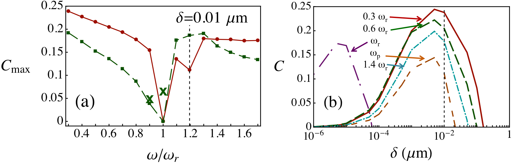
Figure 6: Part (a): $C_{\mathrm{max}}$ vs $\omega/\omega_{r}$ for $\delta=0.01\mu$m. The red curve concerns the case of identical electric dipoles oriented along the $z$ axis and the green along the $x$ axis. The solid (red) and dashed (green) lines just connect the sampled frequencies. Crosses indicate the occurrence of larger values of $C$ at the same frequency but for different values of $\delta$. The black dotted vertical line concerns the frequency $\omega_{p}\simeq 1.2\omega_{r}$. Part (b): $C$ vs $\delta$ for several values of $\omega$ indicated in the figure in the case of identical electric dipoles oriented along the z-axis.

The values of the parameters corresponding to each maximum vary with frequency. The best configuration is always characterized by values of $n(\omega,T_{\mathrm{W}})$ close to zero and $n(\omega,T_{\mathrm{M}})$ between 1 and 3. Smaller values of $n(\omega,T_{\mathrm{M}})$ are needed in the green curve. The zone where to place the qubits is around 1 $\mu$m from the slab at $0.3\,\omega_{r}$, gradually decreasing (specially after $\omega_{r}$) down to 0.25 $\mu$m at $1.7\,\omega_{r}$. For the red curve the best choice is always $z_{1}$ close to $z_{2}$ (in our numerical sample, we limit the minimal distance at the order of 0.1 $\mu$m) and $r_{12}=0$, while for the green curve it is $z_{1}=z_{2}$ and $r_{12}$ small (of the order of 0.01 $\mu$m). This means that the best configuration is when the interatomic axis is aligned with dipoles direction. For $\omega$ around $\omega_{p}$ we point out the occurrence of larger values of $C$ for different values of $\delta$, points indicated with a cross above the green curve. In the absence of large values of $C$ in correspondence to the canonical choice of the parameters described above, small values of $C$ become evident for a different set of parameters. This corresponds to larger values of $\delta$ (of the order of $1\mu$m or more), $z_{1}\simeq 2\mu$m, $z_{2}\simeq 4\mu$m and $r_{12}\simeq 0.5\mu$m. In part (b), we plot the dependence of $C$ on $\delta$ for several values of $\omega$ as indicated in the figure. The maximum of $C$ is always obtained close to $\delta=0.01\mu$m, which is the value chosen in part (a), except around $\omega_{r}$ where much smaller values of $\delta$ are required. This explains why in part (a) concurrence decreases around $\omega_{r}$ for $\delta=0.01\mu$m.

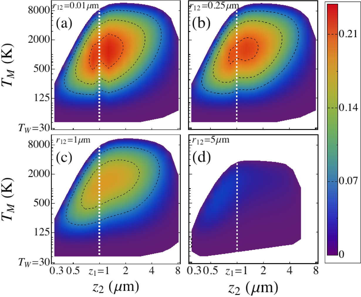
Figure 7: Density plot of $C$ vs $z_{2}$ and $T_{\mathrm{M}}$, for four different values of $r_{12}$: 0.01 $\mu$m (a), 0.25 $\mu$m (b), 1 $\mu$m (c) and 5 $\mu$m (d). The other parameters are $z_{1}{\simeq 1.04}\,\mu$m, $T_{\mathrm{W}}=30$ K, $\omega=0.3\,\omega_{r}$, $\delta=0.01\mu$m. The white zones correspond to $C=0$. The two electric dipoles are identical and perpendicular to the slab. The white lines correspond to the case $z_{2}=z_{1}$.

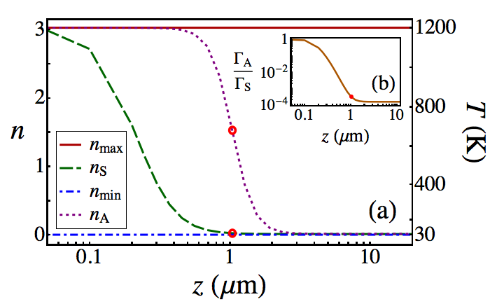
Figure 8: $n_{\mathrm{S}}$, $n_{\mathrm{A}}$, $n_{min}=n(0.3\omega_{r},T_{\mathrm{W}})$, $n_{max}=n(0.3\omega_{r},T_{\mathrm{M}})$, and $\Gamma_{\mathrm{A}}/\Gamma_{\mathrm{S}}$ (inset) vs $z=z_{1}=z_{2}.$ Values of paramters: $T_{\mathrm{W}}=30$ K, $T_{\mathrm{M}}=1200$ K, $\delta=0.01\,\mu$m and $r_{12}$=0.25 $\mu$m. The two electric dipoles are identical and perpendicular to the slab. The temperatures corresponding to the values of $n$ are also indicated.

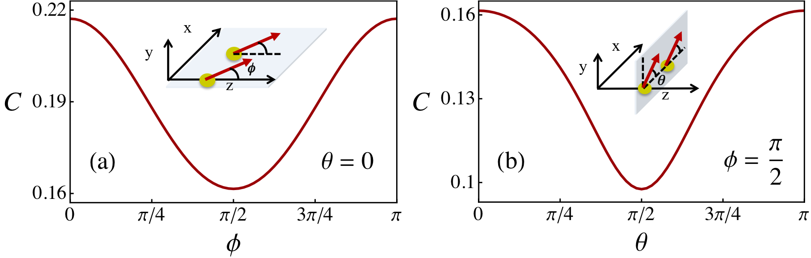
Figure 9: Part (a): $C$ vs $\phi$, angle formed between the dipole directions and the $z$ axis (see inset), in the case $\theta=0$ ($\theta$ is the angle between the projection of dipole directions in the $xy$ plane and the $x$ axis). Part (b): $C$ vs $\theta$ (see inset) in the case $\phi=\pi/2$ (dipole directions in the $xy$ plane). Values of parameters: $T_{\mathrm{W}}=30$ K, $T_{\mathrm{M}}=1200$ K, $\delta=0.01\mu$m, $z=z_{1}=z_{2}{\simeq 1.04}\,\mu$m and $r_{12}$=0.25 $\mu$m.

In figure 7 we plot the steady concurrence as a function of the position of the second qubit $z_{2}$ and of the slab temperature $T_{\mathrm{M}}$ for four different values of $r_{12}$. From (a) to (d) the two-qubit distance $[r_{12}^{2}+(z_{1}-z_{2})^{2}]^{1/2}$ increases leading to a progressive decrease of the values of concurrence generated. A maximum of $C\simeq 0.24$ is obtained in part (a) for $z_{2}\simeq 1.3\mu$m and $T_{\mathrm{M}}\simeq 1100$ K. The white lines correspond to the case $z_{2}=z_{1}$ for which equation (54) holds for concurrence. In part (a), the maximum along the white curve is $C\sim 0.222$ in correspondence to $\Gamma_{\mathrm{A}}/\Gamma_{\mathrm{S}}\sim 4.6\times 10^{-7}$, $n_{\mathrm{S}}\sim 0.02$ and $n_{\mathrm{A}}\sim 1.56$ which correspond to effective temperatures for the two decay channels $T_{\mathrm{S}}\sim 90$ K and $T_{\mathrm{A}}\sim 690$ K. We observe that very high temperatures are considered in this plot only to highlight the entire region where steady entanglement is present. At unphysical temperatures (e.g. above the melting temperature), the plot is only indicative of what would occur if a different material was chosen such that similar values of $\varepsilon(\omega)$ [for SiC it is $\varepsilon(0.3\,\omega_{r})\sim 10.3+0.00721i$] were encountered at lower frequencies. In this case, a similar behavior for steady concurrence at lower temperatures is expected. However, we remark that in our case values of $C$ higher than 0.14 are already present at $T_{\mathrm{M}}\simeq 500$ K in part (a).

In figure 8 we discuss the behavior of $n_{\mathrm{S}}$, $n_{\mathrm{A}}$ and $\Gamma_{\mathrm{A}}/\Gamma_{\mathrm{S}}$, appearing in (54), as a function of $z$. We plot in part (a) $n_{\mathrm{S}}$ and $n_{\mathrm{A}}$ as a function of $z=z_{1}=z_{2}$ and compare them with the value of $n(\omega,T)$ computed at the minimal (here $T_{\mathrm{W}}=30$ K) and maximal (here $T_{\mathrm{M}}=1200$ K) temperature considered. The temperatures and the other parameters are equal to the ones giving the maximum of concurrence in figure 7 (b) along the white line. In the inset [part (b)] we plot $\Gamma_{\mathrm{A}}/\Gamma_{\mathrm{S}}$ as a function of $z=z_{1}=z_{2}$. The plot evidences that near $z\simeq 1\mu$m, both conditions to reach high values of $C$ are satisfied: small values of $n_{\mathrm{S}}$ and $\Gamma_{\mathrm{A}}/\Gamma_{\mathrm{S}}$ in correspondence with high enough values of $n_{\mathrm{A}}$ (see also figure 5 for a comparison).

In figure 9, we analyze the dependence of steady concurrence on dipole orientations. In general, higher results are obtained when the the two dipoles are parallel. We use again the set of parameters corresponding to the maximum in figure 7 (b) along the white line, which is obtained for dipoles along the $z$ axis. We show how concurrence decreases by changing the dipole directions towards the $x$ axis [part (a)] always lying on the $xz$ plane and then towards the $y$ axis [part (b)] always lying one the $xy$ [see insets in Figs. 9 (a)-(b)]. From part (b) it emerges that aligning the dipoles direction to the interatomic axis (which here is the $x$ axis) is the optimal choice in the $xy$ plane inducing a lack of symmetry in this plane between the $x$ and $y$ directions.

6.2 Dynamics

Here we discuss the dynamical behavior of two-qubit density matrix elements and concurrence out of thermal equilibrium, also making comparisons with the thermal equilibrium case. This analysis is performed by solving numerically the evolution governed by (41).

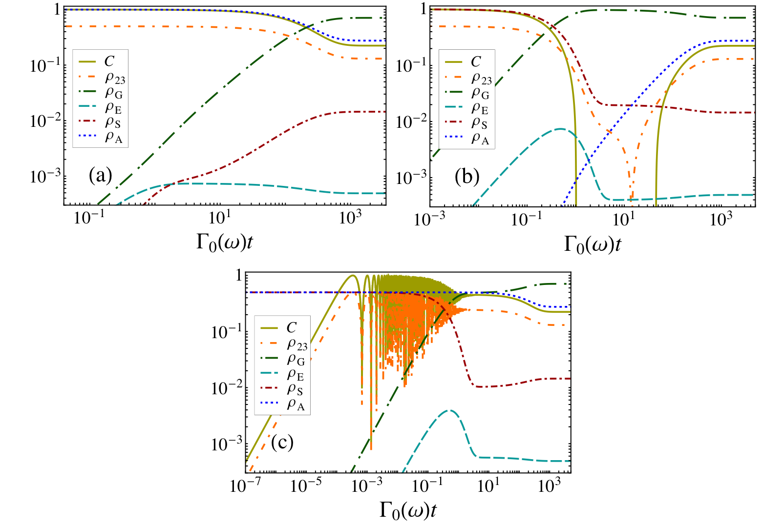
Figure 10: $C$, $\rho_{\mathrm{23}}$, $\rho_{\mathrm{G}}$, $\rho_{\mathrm{E}}$, $\rho_{\mathrm{S}}$ and $\rho_{\mathrm{A}}$ (as indicated in the legend) vs dimensionless time $\Gamma_{0}(\omega)t$ in the case in which the two qubits are initially prepared in the antisymmetric state $|\mathrm{A}\rangle$ [part (a)], the symmetric state $|\mathrm{S}\rangle$ [part (b)] and the factorized state $|\mathrm{2}\rangle$ [part (c)]. The parameters are fixed as $T_{\mathrm{W}}=30$ K, $T_{\mathrm{M}}=1300$ K, $\delta=0.01\mu$m, $z_{1}{\simeq 1.04}\,\mu$m, $z_{2}\simeq 1.28\,\mu$m, $r_{12}$=0.25 $\mu$m and $\omega=0.3\omega_{r}$. The two electric dipoles are identical and perpendicular to the slab.

In figure 10 we plot several density matrix elements and concurrence as a function of dimensionless time $\Gamma_{0}(\omega)t$. Parts (a) and (b) concern the case of maximally entangled initial states, respectively the antisymmetric state $|\mathrm{A}\rangle$ in (a) and the symmetric $|\mathrm{S}\rangle$ in (b) (see values of parameters in the caption of the figure). A quite different dynamical behavior is pointed out. While starting from $|\mathrm{A}\rangle$ entanglement is just preserved at an high value, starting from $|\mathrm{S}\rangle$ concurrence first decreases (going to zero) mainly because of the decrease of $\rho_{\mathrm{S}}$ and then revives because of the increase of $\rho_{\mathrm{A}}$. Dynamical creation of entanglement is yet more evident in part (c) where the initial state is the factorized state $|2\rangle$. In this case, concurrence is initially zero and increases because of the mediated interaction between qubits. Oscillations of $C$ and $\rho_{23}$ are linked to the behavior of $\rho_{\mathrm{AS}(\mathrm{SA})}$ which rapidly oscillate [see (51)] because of the large value of $\Lambda^{12}(\omega)$ which here is equal to $\Lambda^{12}(\omega)/\Gamma_{0}(\omega)\simeq-2.3\times{10^{3}}$. The oscillations are present because $\rho_{\mathrm{AS}(\mathrm{SA})}$ are initially populated [$\rho_{\mathrm{AS}(\mathrm{SA})}=1/2$] while they are not in the cases plotted in parts (a) and (b). States $|\mathrm{S}\rangle$ and $|\mathrm{A}\rangle$ are initially equally populated and become different asymptotically.

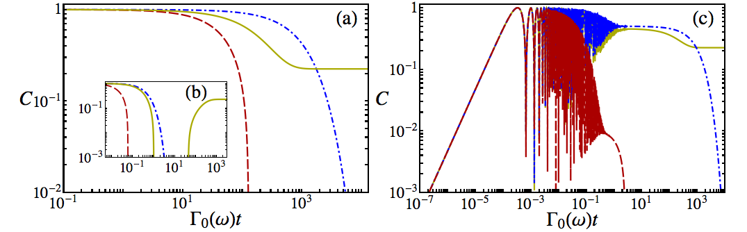
Figure 11: Comparison of the dynamics of concurrence in and out of thermal equilibrium. Concurrence vs dimensionless time $\Gamma_{0}(\omega)t$ in the case in which the two qubits are initially prepared in the antisymmetric state $|\mathrm{A}\rangle$ [part (a)], the symmetric state $|\mathrm{S}\rangle$ [part (b)] and the factorized state $|\mathrm{2}\rangle$ [part (c)]. The red (dashed) and blue (dotdashed) lines regard thermal equilibrium configurations at, respectively, $T_{\mathrm{max}}=T_{\mathrm{W}}=T_{\mathrm{M}}=1300$ K and $T_{\mathrm{min}}=T_{\mathrm{W}}=T_{\mathrm{M}}=30$ K while the yellow (continuous) line the out of thermal equilibrium case $T_{\mathrm{W}}=30$ K and $T_{\mathrm{M}}=1300$ K. The other parameters are fixed as $\delta=0.01\mu$m, $z_{1}{\simeq 1.04}\,\mu$m, $z_{2}{\simeq}1.28\,\mu$m, $r_{12}$=0.25 $\mu$m and $\omega=0.3\omega_{r}$. The two electric dipoles are identical and perpendicular to the slab.

In figure 11 we compare the evolution of concurrence out of thermal equilibrium with the evolutions at equilibrium at the minimal temperature $T_{\mathrm{min}}=T_{\mathrm{W}}=T_{\mathrm{M}}=30$ K and at the maximal temperature $T_{\mathrm{max}}=T_{\mathrm{W}}=T_{\mathrm{M}}=1300$ K. Two initial maximally entangled configurations are compared, the antisymmetric state $|\mathrm{A}\rangle$ in part (a) and the symmetric state $|\mathrm{S}\rangle$ in part (b). At thermal equilibrium concurrence vanishes on shorter times by increasing the temperature, while out of equilibrium steady entanglement is present. At equilibrium, a larger decay time is observed by starting from the antisymmetric state (see also figure 12 on this subject). In part (b), out of equilibrium, concurrence decays on the same equilibrium time scale, the two-qubit state becoming separable, but it reemerges successively. Both in (a) and (b) a large amount of the initial entanglement is thus asymptotically preserved. In part (c) the initial state is the factorized state $|2\rangle$. The main difference here is that concurrence presents strong oscillations [see comment on part (c) of figure 10]. At thermal equilibrium entanglement eventually vanishes on a time scale similar to the one of part (a), while out of equilibrium it is maintained after its creation.

In figure 12, we discuss the dependence of super and sub radiant effects from the presence/absence of thermal equilibrium. Here, super and sub radiance are connected to the occurrence of a decay rate larger or smaller than the one observed in the case of independent qubits, phenomenon due to the interaction of the qubits with a common environment and which depend on the nature of their initial state [27]. In particular, we compare the evolution of the ground state population $\rho_{\mathrm{G}}$ starting from $|\mathrm{S}\rangle$ and $|\mathrm{A}\rangle$ for two different values of $r_{12}$ (0.25 $\mu$m and 15 $\mu$m) at thermal equilibrium at $T_{\mathrm{W}}=T_{\mathrm{M}}=100$ K [part (a)] and at $T_{\mathrm{W}}=T_{\mathrm{M}}=800$ K [part (b)] and out of thermal equilibrium for $T_{\mathrm{W}}=100$ K, $T_{\mathrm{M}}=800$ K [part (c)]. The figure evidences super-radiant behavior when the initial state is $|\mathrm{S}\rangle$ and sub-radiant when it is $|\mathrm{A}\rangle$. The faster or slower increase of $\rho_{\mathrm{G}}$ is due to the role of $\Gamma_{12}(\pm\omega)$ which in the two channel decay rates of (49) is summed to $\Gamma(\pm\omega)$ in the $|\mathrm{S}\rangle$ case and subtracted in the $|\mathrm{A}\rangle$ case. By increasing the value of $r_{12}$, $\Gamma_{12}(\pm\omega)$ decreases and the decay rates $\Gamma^{\mathrm{p(m)}}_{\mathrm{A}}$ and $\Gamma^{\mathrm{p(m)}}_{\mathrm{S}}$, defined in the caption of figure 4, tend both to the same value $\Gamma(+(-)\omega)/\Gamma_{0}(\omega)$, which is the decay rate in the case of single emitters. At thermal equilibrium the asymptotic state is independent on the values of $r_{12}$ while this is not the case out of thermal equilibrium, as pointed out in part (c).

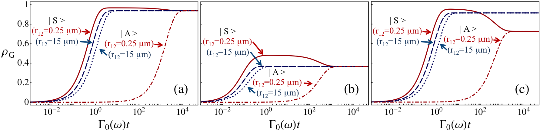
Figure 12: Evolution of $\rho_{G}$ starting from $|\mathrm{S}\rangle$ and $|\mathrm{A}\rangle$ for two different values of $r_{12}$ [$r_{12}$=0.25 $\mu$m or $r_{12}$=15 $\mu$m]. Part (a): thermal equilibrium at $T_{\mathrm{W}}=T_{\mathrm{M}}=100$ K. Part (b): thermal equilibrium at $T_{\mathrm{W}}=T_{\mathrm{M}}=800$ K. Part (c): out of thermal equilibrium, $T_{\mathrm{W}}=100$ K and $T_{\mathrm{M}}=800$ K. Other parameters $\delta=0.01\mu$m, $z=z_{1}=z_{2}{\simeq 1.04}\,\mu$m and $\omega=0.3\omega_{r}$. The two electric dipoles are identical and perpendicular to the slab. The assumptions made in Sec. 5.4 are thus satisfied.

We finally remark that relevant differences are expected when the Markovian and the rotating wave approximation, here adopted, are not valid. In the non-Markovian regime another source of oscillations in the dynamics of concurrence typically emerges [13], while the effect of counter rotating terms is known to modify the creation of entanglement between the two emitters [61].

7 Conclusions

In this paper we have investigated a system made of two quantum emitters interacting with a common stationary electromagnetic field out of thermal equilibrium generated by an arbitrary body and by the surrounding walls held at fixed different temperatures. The environmental field is characterized by means of its correlation functions out of equilibrium which also depend on the scattering properties of the body. We have derived the expressions in the absence of thermal equilibrium of the various functions governing the dissipative dynamics of the two emitters and compared them with the ones holding at thermal equilibrium. This has been done in the case of emitters characterized by an arbitrary number of levels. We have then specialized our investigation to the case of two qubits discussing the new features emerging out of thermal equilibrium.

For a restricted parameter region we have analytically shown that absence of equilibrium may lead to the generation of steady entangled states. This phenomenon has been interpreted in terms of different effective temperatures associated to two decay channels connecting the total excited and ground states via the symmetric and antisymmetric states respectively. The two-qubit dynamics can be directed towards mixed states where the antisymmetric contribution is larger than the symmetric one (or viceversa), resulting in the presence of steady entanglement. It has been found in this specific case a value of 1/3 as maximum for the concurrence, quantifying the steady entanglement.

We have then numerically investigated the general dependence of steady states and dynamics on the various parameters, without any restriction on the decay rates, in the case the body placed in proximity of the two qubits is a slab made of SiC. The dependence of steady entanglement on the two-qubit distance, their common transition frequency with respect to the slab resonances, the slab thickness, the dipoles orientations and the two involved temperatures has been discussed. Values of concurrence up to 0.24 have been found. Protection and/or generation of entanglement according to the nature of the two-qubit initial state, entangled or not, have been pointed out, also comparing entanglement dynamics in the presence or absence of thermal equilibrium. Higher values of steady concurrence are found for transition frequencies far from the slab resonances ($\omega/\omega_{r}=0.3$) and small thickness ($\delta\simeq 0.01\mu$m). Remarkably, steady entanglement can be obtained starting from configurations at thermal equilibrium and by increasing one of the two temperatures involved in the environment of the two qubits.

The possibility to observe the effects we discussed could be explored, for example, for emitters made by trapped atoms [43] or by artificial atoms such as quantum dots or superconducting qubits, placed in proximity of a substrate held at a temperature different from that of the cell surrounding the emitters and the substrate.

Appendix A Correlation functions

Here we connect the correlation functions to $T_{\mathrm{M}}$ and $T_{\mathrm{W}}$ and to the properties of the body as well. To this purpose, we first develop the connection between (14) and the correlation functions in frequency space. Using (6) and homogeneity in time, we have

$$\eqalign{\Xi_{ii^{\prime}}^{qq^{\prime}}(\omega)=&\frac{1}{\hbar^{2}}\int_{0}^{\infty}ds\int_{0}^{+\infty}\frac{d\omega^{\prime}}{2\pi}\int_{0}^{+\infty}\frac{d\omega^{\prime\prime}}{2\pi}\Bigl{[}e^{-i(\omega^{\prime\prime}-\omega)s}\langle E_{i}(\mathbf{R}_{q},\omega^{\prime\prime})E_{i^{\prime}}^{\dagger}(\mathbf{R}_{q^{\prime}},\omega^{\prime})\rangle\\ &\,+e^{i(\omega+\omega^{\prime\prime})s}\langle E_{i}^{\dagger}(\mathbf{R}_{q},\omega^{\prime\prime})E_{i^{\prime}}(\mathbf{R}_{q^{\prime}},\omega^{\prime})\rangle\Bigr{]},}$$ (56)

where we have used $\langle E_{i}(\mathbf{R}_{q},\omega^{\prime\prime})E_{i^{\prime}}(\mathbf{R}_{q^{\prime}},\omega^{\prime})\rangle=\langle E_{i}^{\dagger}(\mathbf{R}_{q},\omega^{\prime\prime})E_{i^{\prime}}^{\dagger}(\mathbf{R}_{q^{\prime}},\omega^{\prime})\rangle=0$. By using $\int_{0}^{\infty}ds\exp(-i\epsilon s)=\pi\delta(\epsilon)-i\mathcal{P}\frac{1}{\epsilon}$ (where $\mathcal{P}$ indicate the principal part of the integral), we obtain from previous equation and (14) (we assume $\omega>0$)

$$\eqalign{\gamma_{ii^{\prime}}^{qq^{\prime}}(\omega)=&\frac{1}{\hbar^{2}}\int_{0}^{+\infty}\frac{d\omega^{\prime}}{2\pi}\langle E_{i}(\mathbf{R}_{q},\omega)E_{i^{\prime}}^{\dagger}(\mathbf{R}_{q^{\prime}},\omega^{\prime})\rangle,\\ \gamma_{ii^{\prime}}^{qq^{\prime}}(-\omega)=&\frac{1}{\hbar^{2}}\int_{0}^{+\infty}\frac{d\omega^{\prime}}{2\pi}\langle E_{i}^{\dagger}(\mathbf{R}_{q},\omega)E_{i^{\prime}}(\mathbf{R}_{q^{\prime}},\omega^{\prime})\rangle,\\ s_{ii^{\prime}}^{qq^{\prime}}(\omega)=&\frac{1}{\hbar^{2}}\mathcal{P}\int_{0}^{+\infty}\frac{d\omega^{\prime}}{2\pi}\int_{0}^{+\infty}\frac{d\omega^{\prime\prime}}{2\pi}\Bigg{[}\frac{\langle E_{i}(\mathbf{R}_{q},\omega^{\prime\prime})E_{i^{\prime}}^{\dagger}(\mathbf{R}_{q^{\prime}},\omega^{\prime})\rangle}{\omega-\omega^{\prime\prime}}\\ &+\frac{\langle E_{i}^{\dagger}(\mathbf{R}_{q},\omega^{\prime\prime})E_{i^{\prime}}(\mathbf{R}_{q^{\prime}},\omega^{\prime})\rangle}{\omega+\omega^{\prime\prime}}\Bigg{]}.}$$ (57)

By using the decomposition in (7), we obtain

$$\eqalign{&\langle E_{i}(\mathbf{R}_{q},\omega)E_{i^{\prime}}^{\dagger}(\mathbf{R}_{q^{\prime}},\omega^{\prime})\rangle=\sum_{\phi,\phi^{\prime},p,p^{\prime}}\int\frac{d^{2}\mathbf{k}}{(2\pi)^{2}}\int\frac{d^{2}\mathbf{k}^{\prime}}{(2\pi)^{2}}e^{i(\mathbf{K}^{\phi}\cdot\mathbf{R}_{q}-\mathbf{K^{\prime}}^{\phi^{\prime}*}\cdot\mathbf{R}_{q^{\prime}})}\\ &\,\times[\hat{\mbox{\boldmath$\epsilon$}}_{p}^{\phi}(\mathbf{k},\omega)]_{i}[\hat{\mbox{\boldmath$\epsilon$}}_{p^{\prime}}^{\phi^{\prime}}(\mathbf{k}^{\prime},\omega^{\prime})]_{i^{\prime}}^{*}\langle E_{p}^{\phi}(\mathbf{k},\omega)E_{p^{\prime}}^{\phi^{\prime}{\dagger}}(\mathbf{k}^{\prime},\omega^{\prime})\rangle,}$$ (58)

and

$$\eqalign{&\langle E_{i}^{\dagger}(\mathbf{R}_{q},\omega)E_{i^{\prime}}(\mathbf{R}_{q^{\prime}},\omega^{\prime})\rangle=\sum_{\phi,\phi^{\prime},p,p^{\prime}}\int\frac{d^{2}\mathbf{k}}{(2\pi)^{2}}\int\frac{d^{2}\mathbf{k}^{\prime}}{(2\pi)^{2}}e^{-i(\mathbf{K}^{\phi*}\cdot\mathbf{R}_{q}-\mathbf{K^{\prime}}^{\phi^{\prime}}\cdot\mathbf{R}_{q^{\prime}})}\\ &\times[\hat{\mbox{\boldmath$\epsilon$}}_{p}^{\phi}(\mathbf{k},\omega)]_{i}^{*}[\hat{\mbox{\boldmath$\epsilon$}}_{p^{\prime}}^{\phi^{\prime}}(\mathbf{k}^{\prime},\omega^{\prime})]_{i^{\prime}}\langle E_{p}^{\phi{\dagger}}(\mathbf{k},\omega)E_{p^{\prime}}^{\phi^{\prime}}(\mathbf{k}^{\prime},\omega^{\prime})\rangle,}$$ (59)

where $\omega>0$. We observe that last equation can be obtained by taking the complex conjugate of (58) after having interchanged the operators $E_{p}^{\phi}(\mathbf{k},\omega)$ and $E_{p^{\prime}}^{\phi^{\prime}{\dagger}}(\mathbf{k}^{\prime},\omega^{\prime})$.

We now combine equations (18) and (19) to obtain the symmetrized correlation functions of the amplitude operator of the total field in the region of interest

$$\eqalign{&\langle E^{+}_{p}(\mathbf{k},\omega)E^{+{\dagger}}_{p^{\prime}}(\mathbf{k}^{\prime},\omega^{\prime})\rangle_{\mathrm{sym}}=2\pi\delta(\omega-\omega^{\prime})\frac{\omega}{2\epsilon_{0}c^{2}}\langle p,\mathbf{k}|\Bigl{[}N(\omega,T_{\mathrm{M}})\Bigl{(}\mathcal{P}_{-1}^{\mathrm{(pw)}}-\mathcal{R}\mathcal{P}_{-1}^{\mathrm{(pw)}}\mathcal{R}^{{\dagger}}\\ &\,+\mathcal{R}\mathcal{P}_{-1}^{\mathrm{(ew)}}-\mathcal{P}_{-1}^{\mathrm{(ew)}}\mathcal{R}^{{\dagger}}-\mathcal{T}\mathcal{P}_{-1}^{\mathrm{(pw)}}\mathcal{T}^{{\dagger}}\Bigr{)}+N(\omega,T_{\mathrm{W}})\Bigl{(}\mathcal{T}\mathcal{P}_{-1}^{\mathrm{(pw)}}\mathcal{T}^{{\dagger}}+\mathcal{R}\mathcal{P}_{-1}^{\mathrm{(pw)}}\mathcal{R}^{{\dagger}}\Bigr{)}\Bigr{]}|p^{\prime},\mathbf{k}^{\prime}\rangle,\\ &\langle E^{+}_{p}(\mathbf{k},\omega)E^{-{\dagger}}_{p^{\prime}}(\mathbf{k}^{\prime},\omega^{\prime})\rangle_{\mathrm{sym}}=2\pi\delta(\omega-\omega^{\prime})\frac{\omega}{2\epsilon_{0}c^{2}}N(\omega,T_{\mathrm{W}})\langle p,\mathbf{k}|\mathcal{R}\mathcal{P}_{-1}^{\mathrm{(pw)}}|p^{\prime},\mathbf{k}^{\prime}\rangle,\\ &\langle E^{-}_{p}(\mathbf{k},\omega)E^{+{\dagger}}_{p^{\prime}}(\mathbf{k}^{\prime},\omega^{\prime})\rangle_{\mathrm{sym}}=2\pi\delta(\omega-\omega^{\prime})\frac{\omega}{2\epsilon_{0}c^{2}}N(\omega,T_{\mathrm{W}})\langle p,\mathbf{k}|\mathcal{P}_{-1}^{\mathrm{(pw)}}\mathcal{R}^{{\dagger}}|p^{\prime},\mathbf{k}^{\prime}\rangle,\\ &\langle E^{-}_{p}(\mathbf{k},\omega)E^{-{\dagger}}_{p^{\prime}}(\mathbf{k}^{\prime},\omega^{\prime})\rangle_{\mathrm{sym}}=2\pi\delta(\omega-\omega^{\prime})\frac{\omega}{2\epsilon_{0}c^{2}}N(\omega,T_{\mathrm{W}})\langle p,\mathbf{k}|\mathcal{P}_{-1}^{\mathrm{(pw)}}|p^{\prime},\mathbf{k}^{\prime}\rangle.}$$ (60)

However, in order to develop equations (58) and (59) we need the non-symmetrized versions of these correlation functions. To compute them, we first remark that the source correlation functions reported in (19) have been derived using thermal-equilibrium techniques at the temperature of each source individually (see [48] for a detailed discussion). It follows that we can use Kubo’s prescription [53], according to which in order to obtain $\langle AB\rangle$ from $\langle AB\rangle_{\mathrm{sym}}$ the replacement $N(\omega,T_{i})\rightarrow\hbar\omega\bigl{[}1+n(\omega,T_{i})\bigr{]}$ must be performed, whilst $\langle BA\rangle$ results from the replacement $N(\omega,T_{i})\rightarrow\hbar\omega\,n(\omega,T_{i})$.

Using (60) in (58) we obtain for the antinormally ordered correlation functions, the form

$$\eqalign{\langle E_{i}&(\mathbf{R}_{q},\omega)E_{i^{\prime}}^{\dagger}(\mathbf{R}_{q^{\prime}},\omega^{\prime})\rangle=2\pi\delta(\omega-\omega^{\prime})\langle E_{i}(\mathbf{R}_{q},\omega)E_{i^{\prime}}^{\dagger}(\mathbf{R}_{q^{\prime}},\omega)\rangle,}$$ (61)

being

$$\eqalign{&\langle E_{i}(\mathbf{R}_{q},\omega)E_{i^{\prime}}^{\dagger}(\mathbf{R}_{q^{\prime}},\omega)\rangle=\frac{\hbar\omega^{2}}{2\epsilon_{0}c^{2}}\sum_{p,p^{\prime}}\int\frac{d^{2}\mathbf{k}}{(2\pi)^{2}}\int\frac{d^{2}\mathbf{k}^{\prime}}{(2\pi)^{2}}e^{i(\mathbf{k}\cdot\mathbf{r}_{q}-\mathbf{k}^{\prime}\cdot\mathbf{r}_{q^{\prime}})}\\ &\,\times\langle p,\mathbf{k}|\Bigl{\{}e^{i(k_{z}z_{q}-k_{z}^{{}^{\prime}*}z_{q^{\prime}})}[\hat{\mbox{\boldmath$\epsilon$}}_{p}^{+}(\mathbf{k},\omega)]_{i}[\hat{\mbox{\boldmath$\epsilon$}}_{p^{\prime}}^{+}(\mathbf{k}^{\prime},\omega)]_{i^{\prime}}^{*}\Bigl{[}\bigl{[}1+n(\omega,T_{\mathrm{M}})\bigr{]}\\ &\,\times\Bigl{(}\mathcal{P}_{-1}^{\mathrm{(pw)}}-\mathcal{R}\mathcal{P}_{-1}^{\mathrm{(pw)}}\mathcal{R}^{{\dagger}}+\mathcal{R}\mathcal{P}_{-1}^{\mathrm{(ew)}}-\mathcal{P}_{-1}^{\mathrm{(ew)}}\mathcal{R}^{{\dagger}}-\mathcal{T}\mathcal{P}_{-1}^{\mathrm{(pw)}}\mathcal{T}^{{\dagger}}\Bigr{)}+\bigl{[}1+n(\omega,T_{\mathrm{W}})\bigr{]}\\ &\,\times\Bigl{(}\mathcal{T}\mathcal{P}_{-1}^{\mathrm{(pw)}}\mathcal{T}^{{\dagger}}+\mathcal{R}\mathcal{P}_{-1}^{\mathrm{(pw)}}\mathcal{R}^{{\dagger}}\Bigr{)}\Bigr{]}+\bigl{[}1+n(\omega,T_{\mathrm{W}})\bigr{]}\Bigl{[}e^{i(k_{z}z_{q}+k_{z}^{{}^{\prime}*}z_{q^{\prime}})}\\ &\,\times[\hat{\mbox{\boldmath$\epsilon$}}_{p}^{+}(\mathbf{k},\omega)]_{i}[\hat{\mbox{\boldmath$\epsilon$}}_{p^{\prime}}^{-}(\mathbf{k}^{\prime},\omega)]_{i^{\prime}}^{*}\mathcal{R}\mathcal{P}_{-1}^{\mathrm{(pw)}}+e^{-i(k_{z}z_{q}+k_{z}^{{}^{\prime}*}z_{q^{\prime}})}[\hat{\mbox{\boldmath$\epsilon$}}_{p}^{-}(\mathbf{k},\omega)]_{i}[\hat{\mbox{\boldmath$\epsilon$}}_{p^{\prime}}^{+}(\mathbf{k}^{\prime},\omega)]_{i^{\prime}}^{*}\\ &\,\times\mathcal{P}_{-1}^{\mathrm{(pw)}}\mathcal{R}^{{\dagger}}+e^{-i(k_{z}z_{q}-k_{z}^{{}^{\prime}*}z_{q^{\prime}})}[\hat{\mbox{\boldmath$\epsilon$}}_{p}^{-}(\mathbf{k},\omega)]_{i}[\hat{\mbox{\boldmath$\epsilon$}}_{p^{\prime}}^{-}(\mathbf{k}^{\prime},\omega)]_{i^{\prime}}^{*}\mathcal{P}_{-1}^{\mathrm{(pw)}}\Bigr{]}\Big{\}}|p^{\prime},\mathbf{k}^{\prime}\rangle.}$$ (62)

We observe that the normally ordered correlation functions $\langle E_{i}^{\dagger}(\mathbf{R}_{q},\omega)E_{i^{\prime}}(\mathbf{R}_{q^{\prime}},\omega^{\prime})\rangle$ of (59) are obtained from the two previous equations by replacing $\bigl{[}1+n(\omega,T_{i})\bigr{]}$ with $n(\omega,T_{i})$ and by taking the complex conjugate. Equation (57) finally becomes

$$\eqalign{\gamma_{ii^{\prime}}^{qq^{\prime}}(\omega)=&\frac{1}{\hbar^{2}}\langle E_{i}(\mathbf{R}_{q},\omega)E_{i^{\prime}}^{\dagger}(\mathbf{R}_{q^{\prime}},\omega)\rangle,\quad\gamma_{ii^{\prime}}^{qq^{\prime}}(-\omega)=\frac{1}{\hbar^{2}}\langle E_{i}^{\dagger}(\mathbf{R}_{q},\omega)E_{i^{\prime}}(\mathbf{R}_{q^{\prime}},\omega)\rangle,\\ s_{ii^{\prime}}^{qq^{\prime}}(\omega)=&\frac{1}{\hbar^{2}}\mathcal{P}\int_{0}^{+\infty}\frac{d\omega^{\prime}}{2\pi}\Bigg{[}\frac{\langle E_{i}(\mathbf{R}_{q},\omega^{\prime})E_{i^{\prime}}^{\dagger}(\mathbf{R}_{q^{\prime}},\omega^{\prime})\rangle}{\omega-\omega^{\prime}}+\frac{\langle E_{i}^{\dagger}(\mathbf{R}_{q},\omega^{\prime})E_{i^{\prime}}(\mathbf{R}_{q^{\prime}},\omega^{\prime})\rangle}{\omega+\omega^{\prime}}\Bigg{]}.}$$ (63)

Appendix B Absence of matter

Here, we treat explicitly the case when there is no body close to the two emitters. In this case we have in (60) $\mathcal{T}=1$, $\mathcal{R}=0$, or equivalently in (28) $\rho_{p}(\mathbf{k},\omega)=0$ and $\tau_{p}(\mathbf{k},\omega)=1$ [$\varepsilon(\omega)=1$]. It follows that the integral matrices in (37) reduce to $[A^{qq^{\prime}}(\omega)]_{ii^{\prime}}=[B^{qq^{\prime}}(\omega)]_{ii^{\prime}}$ and $[C^{qq^{\prime}}(\omega)]_{ii^{\prime}}=[D^{qq^{\prime}}(\omega)]_{ii^{\prime}}=0$, so that $[\alpha^{qq^{\prime}}_{\mathrm{M}}(\omega)]_{ii^{\prime}}=0$ and $[\alpha^{qq^{\prime}}_{\mathrm{W}}(\omega)]_{ii^{\prime}}$ (we choose the $x$ axis along the inter-atomic axis so that in (33) $z_{q}=z_{q^{\prime}}=0$ and $\mathbf{R_{q}}-\mathbf{R}_{q^{\prime}}=\{r_{qq^{\prime}},0,0\}$):

$$\eqalign{[\alpha^{qq^{\prime}}_{\mathrm{W}}(\omega)]_{ii^{\prime}}=\frac{3c}{4\omega}\sum_{p}\int_{0}^{\frac{\omega}{c}}\frac{k\,dk}{k_{z}}\mathrm{Re}{[N_{p}^{++}(k,\omega)]_{ii^{\prime}}}=(\alpha^{qq^{\prime}}_{\mathrm{W}})_{\parallel}\tilde{e}_{\parallel}+(\alpha_{W})_{\perp}\Bigl{(}\tilde{e}_{\perp(y)}+\tilde{e}_{\perp(z)}\Bigr{)},}$$ (64)

where $\tilde{e}_{\parallel}$, $\tilde{e}_{\perp(y)}$ and $\tilde{e}_{\perp(z)}$ are respectively unit vectors along the parallel and the perpendicular directions to the inter-atomic axe $(x)$ and

$$\eqalign{(\alpha^{qq^{\prime}}_{\mathrm{W}})_{\parallel}=3\Bigl{(}\frac{\sin\tilde{r}}{\tilde{r}^{3}}-\frac{\cos\tilde{r}}{\tilde{r}^{2}}\Bigr{)},\quad(\alpha^{qq^{\prime}}_{\mathrm{W}})_{\perp}=\frac{3}{2}\Bigl{(}\frac{\sin\tilde{r}}{\tilde{r}}+\frac{\cos\tilde{r}}{\tilde{r}^{2}}-\frac{\sin\tilde{r}}{\tilde{r}^{3}}\Bigr{)},}$$ (65)

where $\tilde{\mathbf{r}}=(\mathbf{R_{q}}-\mathbf{R}_{q^{\prime}})\omega/c$ and $\tilde{r}=|\tilde{\mathbf{r}}|$. Using the two previous equations and (63) and (21), $\Gamma^{qq^{\prime}}(\omega)$ of (17) can be cast under the form, by introducing $\hat{\mathbf{r}}=\tilde{\mathbf{r}}/\tilde{r}$,

$$\eqalign{\Gamma^{qq^{\prime}}(\omega)=&\sqrt{\Gamma_{0}^{q}(\omega)\Gamma_{0}^{q^{\prime}}(\omega)}[1+n(\omega,T_{\mathrm{W}})]\Bigl{\{}(\tilde{\mathbf{d}}_{mn}^{q\,*}\cdot{\hat{\bf{r}}})(\tilde{\mathbf{d}}_{m^{\prime}n^{\prime}}^{q^{\prime}}\cdot{\hat{\bf{r}}})(\alpha^{qq^{\prime}}_{\mathrm{W}})_{\parallel}\\ &\,+\bigl{[}\tilde{\mathbf{d}}_{mn}^{q\,^{*}}\cdot\tilde{\mathbf{d}}_{m^{\prime}n^{\prime}}^{q^{\prime}}-(\tilde{\mathbf{d}}_{mn}^{q\,*}\cdot{\hat{\bf{r}}})\;(\tilde{\mathbf{d}}_{m^{\prime}n^{\prime}}^{q^{\prime}}\cdot{\hat{\bf{r}}})\bigr{]}(\alpha^{qq^{\prime}}_{\mathrm{W}})_{\perp}\Bigr{\}},}$$ (66)

which does not depend anymore on the reference system chosen to derive (65). In order to compare previous result with known expressions, let us consider the case of two qubits in vacuum with dipoles parallel between them (direction $\tilde{\mathbf{d}}$) with different modulus $|\mathbf{d}_{q}|\neq|\mathbf{d}_{q^{\prime}}|$. In this case, previous equation reduces to the form (see for instance [26, 27])

$$\eqalign{\Gamma^{qq^{\prime}}(\omega)&=\sqrt{\Gamma_{0}^{q}(\omega)\Gamma_{0}^{q^{\prime}}(\omega)}[1+n(\omega,T_{\mathrm{W}})]\frac{3}{2}\Bigl{\{}\Bigl{[}1-(\mathbf{\tilde{d}}\cdot{\hat{\mathbf{r}}})^{2}\Bigr{]}\frac{\sin\tilde{r}}{\tilde{r}}\\ &+\Bigl{[}1-3(\mathbf{\tilde{d}}\cdot{\hat{\mathbf{r}}})^{2}\Bigr{]}\Bigl{(}\frac{\cos\tilde{r}}{\tilde{r}^{2}}-\frac{\sin\tilde{r}}{\tilde{r}^{3}}\Bigr{)}\Bigr{\}}.}$$ (67)

Appendix C Green’s function

Here we connect the approaches based on field correlations functions and on Green’s function in order to develop the expression for $\Lambda^{qq^{\prime}}(\omega)$ of (26). At thermal equilibrium the correlators of the total electromagnetic field outside the body follow from the fluctuation-dissipation theorem [55]

$$\eqalign{&\langle E^{\mathrm{(tot)}}_{i}(\mathbf{R}_{q},\omega)E_{i^{\prime}}^{\mathrm{(tot)}{\dagger}}(\mathbf{R}_{q^{\prime}},\omega^{\prime})\rangle=2\pi\delta(\omega-\omega^{\prime})2\hbar[1+n(\omega,T)\Bigr{]}\mathrm{Im}\,G_{ii^{\prime}}(\mathbf{R}_{q},\mathbf{R}_{q^{\prime}},\omega).}$$ (68)

In (68) $G_{ii^{\prime}}(\mathbf{R}_{q},\mathbf{R}_{q^{\prime}},\omega)$ is the $ii^{\prime}$ component of the Green’s function of the system, solution of the differential equation (for two arbitrary points $\mathbf{R}$ and $\mathbf{R}^{\prime}$)

$$\Bigl{[}\nabla_{\mathbf{R}}\times\nabla_{\mathbf{R}}-\frac{\omega^{2}}{c^{2}}\varepsilon(\omega,\mathbf{R})\Bigr{]}\mathbb{G}(\mathbf{R},\mathbf{R}^{\prime},\omega)=\frac{\omega^{2}}{\epsilon_{0}c^{2}}\,\mathbb{I}\,\delta(\mathbf{R}-\mathbf{R}^{\prime})$$ (69)

being $\mathbb{I}$ the identity dyad and $\varepsilon(\omega,\mathbf{R})$ the dielectric function of the medium. The property (68) does not hold in the case of a nonequilibrium configuration. The comparison between (61) and (21) at equilibrium $T_{\mathrm{W}}=T_{\mathrm{M}}=T$, and (68) gives

$$\mathrm{Im}\,G_{ii^{\prime}}(\mathbf{R}_{q},\mathbf{R}_{q^{\prime}},\omega)=\frac{\omega^{3}}{3\pi\epsilon_{0}c^{3}}\frac{[\alpha_{\mathrm{W}}^{qq^{\prime}}(\omega)]_{ii^{\prime}}+[\alpha_{\mathrm{M}}^{qq^{\prime}}(\omega)]_{ii^{\prime}}}{2}.$$ (70)

Once stated this connection, which is used in (26), we need to compute the real part of the Green’s function to develop equation (27). Following appendix C of [48], the $ii^{\prime}$ component of the Green’s function for two arbitrary points $\mathbf{R}=\{\mathbf{r},z\}$ and $\mathbf{R}^{\prime}=\{\mathbf{r}^{\prime},z^{\prime}\}$ on the right side of the body reads like

$$\eqalign{&G_{ii^{\prime}}(\mathbf{R},\mathbf{R}^{\prime},\omega)=G^{(0)}_{ii^{\prime}}(\mathbf{R},\mathbf{R}^{\prime},\omega)+G^{\mathrm{(R)}}_{ii^{\prime}}(\mathbf{R},\mathbf{R}^{\prime},\omega),\\ &G^{(0)}_{ii^{\prime}}(\mathbf{R},\mathbf{R}^{\prime},\omega)=\frac{i\omega^{2}}{2\epsilon_{0}c^{2}}\sum_{p}\int\frac{d^{2}\mathbf{k}}{(2\pi)^{2}}\exp\bigl{[}i\mathbf{k}\cdot\bigl{(}\mathbf{r}-\mathbf{r}^{\prime}\bigr{)}\bigr{]}\frac{1}{k_{z}}\Bigl{[}\theta(z-z^{\prime})[\hat{\mbox{\boldmath$\epsilon$}}^{+}_{p}(\mathbf{k},\omega)]_{i}\\ &\times[\hat{\mbox{\boldmath$\epsilon$}}^{+}_{p}(\mathbf{k},\omega)]_{i^{\prime}}\exp\bigl{[}ik_{z}\bigl{(}z-z^{\prime}\bigr{)}\bigr{]}+\theta(z^{\prime}-z)[\hat{\mbox{\boldmath$\epsilon$}}^{-}_{p}(\mathbf{k},\omega)]_{i}[\hat{\mbox{\boldmath$\epsilon$}}^{-}_{p}(\mathbf{k},\omega)]_{i^{\prime}}\exp\bigl{[}ik_{z}\bigl{(}z^{\prime}-z\bigr{)}\bigr{]}\Bigr{]},\\ &G^{\mathrm{(R)}}_{ii^{\prime}}(\mathbf{R},\mathbf{R}^{\prime},\omega)=\frac{i\omega^{2}}{2\epsilon_{0}c^{2}}\sum_{pp^{\prime}}\int\frac{d^{2}\mathbf{k}}{(2\pi)^{2}}\int\frac{d^{2}\mathbf{k}^{\prime}}{(2\pi)^{2}}\exp\bigl{[}i\bigl{(}\mathbf{k}\cdot\mathbf{r}-\mathbf{k}^{\prime}\cdot\mathbf{r}^{\prime}\bigr{)}\bigr{]}\\ &\times\frac{1}{k^{\prime}_{z}}[\hat{\mbox{\boldmath$\epsilon$}}^{+}_{p}(\mathbf{k},\omega)]_{i}[\hat{\mbox{\boldmath$\epsilon$}}^{-}_{p^{\prime}}(\mathbf{k}^{\prime},\omega)]_{i^{\prime}}\exp\bigl{[}i(k_{z}z+k^{\prime}_{z}z^{\prime}\bigr{)}\bigr{]}\langle\mathbf{k},p|\mathcal{R}|\mathbf{k}^{\prime},p^{\prime}\rangle,}$$ (71)

where $\theta$ is the Heaviside step function [$\theta(x)=1$ for $x>0$ and $\theta(x)=0$ elsewhere] and $G_{ii^{\prime}}(\mathbf{R},\mathbf{R}^{\prime},\omega)$ has been divided in a free term, $G^{(0)}_{ii^{\prime}}(\mathbf{R},\mathbf{R}^{\prime},\omega)$, independent of the scattering operators, and a reflected one, $G^{\mathrm{(R)}}_{ii^{\prime}}(\mathbf{R},\mathbf{R}^{\prime},\omega)$, proportional to $\mathcal{R}$. With regards to the imaginary part of $G_{ii^{\prime}}(\mathbf{R}_{q},\mathbf{R}_{q^{\prime}},\omega)$ it is possible to check starting from (71) that equation (70) is verified.

Concerning the real part of $G_{ii^{\prime}}(\mathbf{R}_{q},\mathbf{R}_{q^{\prime}},\omega)$, to derive its expression we will make use of the properties of the polarization unit vectors,

$$\eqalign{\hat{\mbox{\boldmath$\epsilon$}}_{\mathrm{TE}}^{\phi}(-\mathbf{k},\omega)&=-\hat{\mbox{\boldmath$\epsilon$}}_{\mathrm{TE}}^{\phi}(\mathbf{k},\omega),\quad\hat{\mbox{\boldmath$\epsilon$}}_{\mathrm{TE}}^{-\phi}(\mathbf{k},\omega)=\hat{\mbox{\boldmath$\epsilon$}}_{\mathrm{TE}}^{\phi}(\mathbf{k},\omega),\quad\Bigl{(}\hat{\mbox{\boldmath$\epsilon$}}_{\mathrm{TE}}^{\phi}(\mathbf{k},\omega)\Bigr{)}^{*}=\hat{\mbox{\boldmath$\epsilon$}}_{\mathrm{TE}}^{\phi}(\mathbf{k},\omega),\\ \hat{\mbox{\boldmath$\epsilon$}}_{\mathrm{TM}}^{\phi}(-\mathbf{k},\omega)&=\hat{\mbox{\boldmath$\epsilon$}}_{\mathrm{TM}}^{-\phi}(\mathbf{k},\omega),\quad\Bigl{(}\hat{\mbox{\boldmath$\epsilon$}}_{\mathrm{TM}}^{\phi}(\mathbf{k},\omega)\Bigr{)}^{*}=\cases{\hat{\mbox{\boldmath$\epsilon$}}_{\mathrm{TM}}^{\phi}(\mathbf{k},\omega)&$k_{z}\in\mathbb{R}$\\ \hat{\mbox{\boldmath$\epsilon$}}_{\mathrm{TM}}^{-\phi}(\mathbf{k},\omega)&$k_{z}\notin\mathbb{R}$\\ },}$$ (72)

and of the reciprocity relations of scattering operators presented in appendix D of [48]

$$\frac{1}{k^{{}^{\prime}*}_{z}}(-1)^{p+p^{\prime}}\langle-\mathbf{k}^{\prime},p^{\prime}|\mathcal{R}^{\phi{\dagger}}|-\mathbf{k},p\rangle=\frac{1}{k^{*}_{z}}\langle\mathbf{k},p|\mathcal{R}^{\phi{\dagger}}|\mathbf{k}^{\prime},p^{\prime}\rangle.$$ (73)

Starting from the free term $G^{(0)}_{ii^{\prime}}$ in (71), its real part can be written as the sum of two terms coming, respectively, from the propagative and evanescent sector (a change of variable from $\mathbf{k}$ to $-\mathbf{k}$ is done in the terms obtained by complex conjugation, we make use of (72) and we choose the interatomic axis along the $z$ direction):

$$\eqalign{&\mathrm{Re}\,G^{(0)}_{ii^{\prime}}(\mathbf{R},\mathbf{R}^{\prime},\omega)_{PW}=\frac{i\omega^{2}}{4\epsilon_{0}c^{2}}\frac{1}{(2\pi)^{2}}\int_{0}^{\frac{\omega}{c}}\frac{kdk}{k_{z}}[R(k,\omega)]_{ii^{\prime}}\Bigl{\{}\theta(z-z^{\prime})\Bigl{[}\exp\bigl{[}ik_{z}\bigl{(}z-z^{\prime}\bigr{)}]\\ &\,-\exp\bigl{[}-ik_{z}\bigl{(}z-z^{\prime}\bigr{)}]\Bigr{]}+\theta(z^{\prime}-z)\Bigl{[}\exp\bigl{[}ik_{z}\bigl{(}z^{\prime}-z\bigr{)}\bigr{]}-\exp\bigl{[}-ik_{z}\bigl{(}z^{\prime}-z\bigr{)}\bigr{]}\Bigr{]}\Bigr{\}},\\ &\mathrm{Re}\,G^{(0)}_{ii^{\prime}}(\mathbf{R},\mathbf{R}^{\prime},\omega)_{EW}=\frac{i\omega^{2}}{4\epsilon_{0}c^{2}}\frac{2}{(2\pi)^{2}}\!\int_{\frac{\omega}{c}}^{+\infty}\!\frac{kdk}{k_{z}}[R(k,\omega)]_{ii^{\prime}}\\ &\,\times\Bigl{\{}\theta(z-z^{\prime})\exp\bigl{[}ik_{z}\bigl{(}z-z^{\prime}\bigr{)}]+\theta(z^{\prime}-z)\exp\bigl{[}ik_{z}\bigl{(}z^{\prime}-z\bigr{)}\bigr{]}\Bigr{\}},}$$ (74)

where we have used the angular integrals

$$\eqalign{[R(k,\omega)]_{ii^{\prime}}&=\sum_{p}\int_{0}^{2\pi}d\theta[\hat{\mbox{\boldmath$\epsilon$}}^{+(-)}_{p}(\mathbf{k},\omega)]_{i}[\hat{\mbox{\boldmath$\epsilon$}}^{+(-)}_{p}(\mathbf{k},\omega)]_{i^{\prime}},}$$ (75)

being the matrix $R(k,\omega)$ diagonal with $[R(k,\omega)]_{11}=[R(k,\omega)]_{22}=\pi(2-c^{2}k^{2}/\omega^{2})$ and $[R(k,\omega)]_{33}=2\pi c^{2}k^{2}/\omega^{2}$. The integral in $\mathrm{Re}\,G^{(0)}_{ii^{\prime}}(\mathbf{R},\mathbf{R}^{\prime},\omega)_{PW}$ gives two terms, one erasing exactly the integral in $\mathrm{Re}\,G^{(0)}_{ii^{\prime}}(\mathbf{R},\mathbf{R}^{\prime},\omega)_{EW}$, and the second being equal to (we distinguish diagonal elements perpendicular and parallel to the interatomic axis)

$$\eqalign{&\mathrm{Re}\,G^{(0)}_{\perp}(\mathbf{R},\mathbf{R}^{\prime},\omega)=\frac{1}{4\pi}\frac{\omega^{3}}{\epsilon_{0}c^{3}}\Bigl{[}\frac{(\tilde{r}^{2}-1)\cos\tilde{r}-\tilde{r}\sin\tilde{r}}{\tilde{r}^{3}}\Bigr{]}\\ &\mathrm{Re}\,G^{(0)}_{\parallel}(\mathbf{R},\mathbf{R}^{\prime},\omega)=\frac{1}{2\pi}\frac{\omega^{3}}{\epsilon_{0}c^{3}}\Bigl{[}\frac{\cos\tilde{r}+\tilde{r}\sin\tilde{r}}{\tilde{r}^{3}}\Bigr{]},}$$ (76)

where $\tilde{r}=|\mathbf{R}-\mathbf{R}^{\prime}|\omega/c$ and we named $\mathrm{Re}\,G^{(0)}_{xx}=\mathrm{Re}\,G^{(0)}_{yy}=\mathrm{Re}\,G^{(0)}_{\perp}$ and $\mathrm{Re}\,G^{(0)}_{zz}=\mathrm{Re}\,G^{(0)}_{\parallel}$.

Function $\Lambda^{qq^{\prime}}(\omega)$ of (27) can be thus decomposed in two parts, $\Lambda^{qq^{\prime}}(\omega)=\Lambda_{0}^{qq^{\prime}}(\omega)+\Lambda_{R}^{qq^{\prime}}(\omega)$, connected to $G^{(0)}(\mathbf{R}_{q},\mathbf{R}_{q^{\prime}},\omega)$ and $G^{\mathrm{(R)}}(\mathbf{R}_{q},\mathbf{R}_{q^{\prime}},\omega)$, $\Lambda_{0}^{qq^{\prime}}(\omega)$ being

$$\eqalign{\Lambda_{0}^{qq^{\prime}}(\omega)=&-\sqrt{\Gamma_{0}^{q}(\omega)\Gamma_{0}^{q^{\prime}}(\omega)}\frac{3}{4}\Bigl{\{}\bigl{[}\tilde{\mathbf{d}}_{mn}^{q\,*}\cdot\tilde{\mathbf{d}}_{m^{\prime}n^{\prime}}^{q^{\prime}}-(\tilde{\mathbf{d}}_{mn}^{q\,*}\cdot{\hat{\bf{r}}})\;(\tilde{\mathbf{d}}_{m^{\prime}n^{\prime}}^{q^{\prime}}\cdot{\hat{\bf{r}}})\bigr{]}\\ &\,\times\Bigl{[}\frac{(\tilde{r}^{2}-1)\cos\tilde{r}-\tilde{r}\sin\tilde{r}}{\tilde{r}^{3}}\Bigr{]}+2(\tilde{\mathbf{d}}_{mn}^{q\,^{*}}\cdot{\hat{\bf{r}}})\;(\tilde{\mathbf{d}}_{m^{\prime}n^{\prime}}^{q^{\prime}}\cdot{\hat{\bf{r}}})\Bigl{[}\frac{\cos\tilde{r}+\tilde{r}\sin\tilde{r}}{\tilde{r}^{3}}\Bigr{]}\Bigr{\}},}$$ (77)

which has been put under a form which does not depend anymore on the reference system chosen to derive equation (76). In the case of two qubits in a vacuum field in absence of matter with electric dipoles parallels between them (direction $\tilde{\mathbf{d}}$) with $|\mathbf{d}_{q}|\neq|\mathbf{d}_{q^{\prime}}|$, $\Lambda_{0}^{qq^{\prime}}(\omega)$ of (77) reduces to the known form [26, 27]

$$\eqalign{&\Lambda_{0}^{qq^{\prime}}(\omega)=\sqrt{\Gamma_{0}^{q}(\omega)\Gamma_{0}^{q^{\prime}}(\omega)}\frac{3}{4}\Bigl{\{}\Bigl{[}1-3(\mathbf{\tilde{d}}\cdot{\hat{\mathbf{r}}})^{2}\Bigr{]}\Bigl{(}\frac{\sin\tilde{r}}{\tilde{r}^{2}}+\frac{\cos\tilde{r}}{\tilde{r}^{3}}\Bigr{)}-\Bigl{[}1-(\mathbf{\tilde{d}}\cdot{\hat{\mathbf{r}}})^{2}\Bigr{]}\frac{\cos\tilde{r}}{\tilde{r}}\Bigr{\}},}\\$$ (78)

where we used $\mathbf{\tilde{d}}\cdot{\hat{\mathbf{r}}}=\tilde{d}_{z}$ and $\tilde{d}_{x}^{2}+\tilde{d}_{y}^{2}=1-(\tilde{d}_{z})^{2}$.

We now consider the remaining part of the Green’s function in (71). By making a change of variable in the terms obtained by complex conjugation, $(\mathbf{k},\mathbf{k}^{\prime})\rightarrow(-\mathbf{k},-\mathbf{k}^{\prime})$, and using the reciprocity relations of scattering operators in (73) and the properties of the polarization unit vectors (72), one can obtain

$$\eqalign{&\mathrm{Re}\,G^{(R)}_{ii^{\prime}}(\mathbf{R},\mathbf{R}^{\prime},\omega)=\frac{i\omega^{2}}{4\epsilon_{0}c^{2}}\sum_{p,p^{\prime}}\int\frac{d^{2}\mathbf{k}}{(2\pi)^{2}}\int\frac{d^{2}\mathbf{k}^{\prime}}{(2\pi)^{2}}e^{i(\mathbf{k}\cdot\mathbf{r}-\mathbf{k}^{\prime}\cdot\mathbf{r}^{\prime})}\langle p,\mathbf{k}|\Bigl{\{}e^{i(k_{z}z+k_{z}^{{}^{\prime}*}z^{\prime})}\\ &\,\times[\hat{\mbox{\boldmath$\epsilon$}}_{p}^{+}(\mathbf{k},\omega)]_{i}[\hat{\mbox{\boldmath$\epsilon$}}_{p^{\prime}}^{-}(\mathbf{k}^{\prime},\omega)]_{i^{\prime}}^{*}\mathcal{R}\mathcal{P}_{-1}^{\mathrm{(pw)}}-e^{-i(k_{z}z+k_{z}^{{}^{\prime}*}z^{\prime})}[\hat{\mbox{\boldmath$\epsilon$}}_{p}^{-}(\mathbf{k},\omega)]_{i}[\hat{\mbox{\boldmath$\epsilon$}}_{p^{\prime}}^{+}(\mathbf{k}^{\prime},\omega)]_{i^{\prime}}^{*}\mathcal{P}_{-1}^{\mathrm{(pw)}}\mathcal{R}^{{\dagger}}\\ &\,+e^{i(k_{z}z-k_{z}^{{}^{\prime}*}z^{\prime})}[\hat{\mbox{\boldmath$\epsilon$}}_{p}^{+}(\mathbf{k},\omega)]_{i}[\hat{\mbox{\boldmath$\epsilon$}}_{p^{\prime}}^{+}(\mathbf{k}^{\prime},\omega)]_{i^{\prime}}^{*}\Bigl{(}\mathcal{R}\mathcal{P}_{-1}^{\mathrm{(ew)}}+\mathcal{P}_{-1}^{\mathrm{(ew)}}\mathcal{R}^{{\dagger}}\Bigr{)}\Big{\}}|p^{\prime},\mathbf{k}^{\prime}\rangle.}$$ (79)

References

References

- [1] Werner R F 1989 Phys. Rev. 40 4277
- [2] Amico L, Fazio R, Osterloh A and Vedral V 2008 Rev. Mod. Phys. 80, 517
- [3] Horodecki R et al. 2009 Rev. Mod. Phys. 81 865
- [4] Einstein A, Podolsky B and Rosen N 1935 Phys. Rev. 47 777; Clauser J F, Horne M A, Shimony A and Holt R A 1969 Phys. Rev. Lett. 23 880
- [5] Nielsen M A and Chuang I L 2000 Quantum Computation and Quantum Information (Cambridge: Cambridge University Press)
- [6] L. Masanes, S. Pironio, and A. Acin, Nature Commun. 2, 238 (2011).
- [7] Bennett C H et al. 1993 Phys. Rev. Lett. 70 1895
- [8] Giovannetti V, Lloyd S and Maccone L 2011 Nature Photon. 5 222
- [9] Breuer H P and Petruccione F 2002 The Theory of Open Quantum Systems (Oxford: Oxford University Press)
- [10] Zurek W H 2003 Rev. Mod. Phys. 75 715
- [11] Diósi L 2003 Irreversible Quantum Dynamics ed F Benatti and R Floreanini (Lecture Notes in Physics vol 622) (Berlin: Springer) p 157
- [12] Yu T and Eberly J H 2004 Phys. Rev. Lett. 93 140404
- [13] Bellomo B, Lo Franco R and Compagno G 2007 Phys. Rev. Lett. 99 160502; 2008 Phys. Rev. A 77 032342
- [14] Bellomo B et al. 2010 Phys. Rev. A 81 062309
- [15] Lo Franco R, Bellomo B, Andersson E and Compagno G 2012 Phys. Rev. A 85 032318
- [16] Lidar D A, Chuang I L and Whaley K B 1998 Phys. Rev. Lett. 81 2594
- [17] Bellomo B, Lo Franco R, Maniscalco S and Compagno G 2008 Phys. Rev. A 78 060302(R)
- [18] Maniscalco S et al. 2008 Phys. Rev. Lett. 100 090503
- [19] Plenio M B and Huelga S F 2002 Phys. Rev. Lett. 88 197901
- [20] Verstraete F, Wolf M M and Cirac J I 2009 Nature Phys. 5 633
- [21] Sarlette A, Raimond J M, Brune M and Rouchon P 2011 Phys. Rev. Lett. 107 010402
- [22] Mancini S and Wiseman H M 2007 Phys. Rev. A 75 012330
- [23] Stevenson R N, Hope J J and Carvalho A R R 2011 Phys. Rev. A 84 022332
- [24] Braun D 2002 Phys. Rev. Lett. 89 27790; Benatti F, Floreanini R and Piani M 2003 Phys. Rev. Lett. 91 070402
- [25] Ficek Z and Tanaś R 2008 Phys. Rev. A 77 054301
- [26] Agarwal G S 1974 in Quantum Statistical Theories of Spontaneous Emission and their Relation to other Approaches, edited by G. Höhler, Springer Tracts in Modern Physics Vol. 70 (Berlin: Springer) pp 1-128
- [27] Ficek Z and Swain S 2005 Quantum Interference and Coherence: Theory and Experiments Springer (New York)
- [28] Dzsotjan D, Sorensen S and Fleischhauer M 2010 Phys. Rev. B 82 075427
- [29] González-Tudela A et al. 2011 Phys. Rev. Lett. 106 020501
- [30] Almutairi K., Tanaś R and Ficek Z 2011 Phys. Rev. A 84 013831
- [31] Quiroga L, Rodriguez F J, Ramirez M E and Paris R 2007 Phys. Rev. A 75 032308
- [32] Huang X L, Guo J L and Yi X X 2009 Phys. Rev. A 80 054301
- [33] Camalet S 2011 Eur. Phys. J. B. 84 467
- [34] Z̆nidaric̆ M 2012 Phys. Rev. A 85 012324
- [35] Manzano D, Tiersch M, Asadian A and Briegel H J 2012 Phys. Rev. E 86 061118
- [36] Camalet S 2013 Eur. Phys. J. B. 86 176
- [37] Linden N, Popescu S and Skrzypczyk P 2010 Phys. Rev. Lett. 105 130401
- [38] Brunner N, Linden N, Popescu S and Skrzypczyk P 2012 Phys. Rev. E 85 051117
- [39] Joulain K et al. 2005 Surf. Sci. Rep. 57 59
- [40] Messina R, Antezza M and Ben-Abdallah P 2012 Phys. Rev. Lett. 109 244302
- [41] Antezza M, Pitaevskii L P and Stringari S 2005 Phys. Rev. Lett. 95 113202
- [42] Antezza M 2006 J. Phys. A: Math. Gen. 39 6117
- [43] Obrecht J M et al. 2007 Phys. Rev. Lett. 98 063201
- [44] Antezza M et al. 2008 Phys. Rev. A 77 022901
- [45] Bimonte G 2009 Phys. Rev. A 80 042102
- [46] Krüger M, Emig T and Kardar M 2011 Phys. Rev. Lett. 106 210404
- [47] Messina R and Antezza M 2011 Europhys. Lett. 95 61002
- [48] Messina R and Antezza M 2011 Phys. Rev. A 84 042102
- [49] Bellomo B, Messina R and Antezza M 2012 Europhys. Lett. 100 20006
- [50] Bellomo B, Messina R, Felbacq D and Antezza M 2013 Phys. Rev. A 87 012101
- [51] Bellomo B and Antezza M 2013 Europhys. Lett. 104 10006
- [52] Cohen-Tannoudji C., Dupont-Roc J and Grynberg G 1997 Photons and Atoms: Introduction to Quantum Electrodynamics (Wiley)
- [53] Kubo R 1966 Rep. Prog. Phys. 29 255
- [54] Handbook of Optical Constants of Solids 1998, edited by E. Palik (Academic Press, New York)
- [55] Landau L D and Lifshitz E M 1963 Electrodynamics of Continuous Media (Pergamon Press, Oxford)
- [56] Bellomo B, Lo Franco R and Compagno G Adv. Sci. Lett. 2 459
- [57] Chiuri A, Vallone G, Paternostro M and Mataloni P 2011 Phys. Rev. A 84 020304(R); Di Carlo L et al. 2009 Nature 460 240
- [58] Osborne T J and Nielsen M A 2002 Phys. Rev. A 66 032110; Osterloh A, Amico L, Falci G and Fazio R 2002 Nature 416 608
- [59] Yu T and Eberly J H 2007 Quantum Inf. Comput. 7 459
- [60] Wooters W K 1998 Phys. Rev. Lett. 80 2245
- [61] Wang C and Chen Q-H 2013 New J. Phys. 15 103020