Quantum limit for nuclear spin polarization in semiconductor quantum dots

Abstract

A recent experiment [E. A. Chekhovich et al., Phys. Rev. Lett. 104, 066804 (2010)] has demonstrated that high nuclear spin polarization can be achieved in self-assembled quantum dots by exploiting an optically forbidden transition between a heavy hole and a trion state. However, a fully polarized state is not achieved as expected from a classical rate equation. Here, we theoretically investigate this problem with the help of a quantum master equation and we demonstrate that a fully polarized state cannot be achieved due to formation of a nuclear dark state. Moreover, we show that the maximal degree of polarization depends on structural properties of the quantum dot.

I Introduction

Initialization ono2002 , coherent manipulation petta_science2005 ; koppens_nature2006 ; nowack2007 ; petta2010 ; ribeiro2013 , and readout of a single spin confined in a quantum dot have become a common routine. However, and in spite of all remarkable developed strategies kloeffel2013 , a scalable quantum computer based on spin-qubits loss1998 still faces serious challenges. The main difficulty that has been encountered comes from the unavoidable coupling between the qubit and the surrounding environment. The time evolution of the qubit becomes correlated with the dynamics of the environment degrees of freedom. This would not be a problem in itself if one knew how to control the environment, but in general this cannot be done, and thus the random character (mixed state) of the environment results in the decoherence of the qubit chirolli2008 .

In quantum dots made out of III-V materials, the hyperfine interaction of a single electron with a large number of nuclear spins ($10^{4}$ – $10^{6}$) is the main source of decoherence coish_statsolidi2009 ; petta_science2005 ; koppens_nature2006 ; khaetskii_prl2002 ; merkulov_prb2002 . However, through an extensive effort aiming at prolonging the spin coherence in quantum dots nanostructure, several approaches have been put forward to minimize or even cancel the effects due to nuclear spin induced dynamics. Dynamical decoupling techniques, such as Hahn echo hahn1950 or Carr-Purcell carr1954 , allow a refocusing of the qubit phase by eliminating the low-frequency components of the nuclear spin bath fluctuations. These methods have demonstrated that it is possible to extend the inhomogeneous dephasing time $T_{2}^{*}\sim\,10\,\mathrm{ns}$ petta_science2005 ; koppens_nature2006 ; coish_prb2004 ; coish2005 ; xu2009 up to the dephasing time $T_{2}\sim\,3\,\mathrm{\mu s}$ petta_science2005 ; koppens_nature2006 ; greilich2009 ; clark2009 ; press2010 , which corresponds to the limit imposed by nuclear spin diffusion coish_prb2004 ; witzel2006 . A more recent experiment in gate defined double quantum dots has even revealed $T_{2}\simeq 200\,\mathrm{\mu s}$ bluhm2011 .

Another possible route consists in polarizing the nuclear spins. However, a substantial degree of polarization (close to 100%) is needed coish_prb2004 to increase coherence times. Highly polarized nuclear states are also desirable for other useful tasks in quantum information. Ultimately they can be used as a quantum memory to store the coherent state of the electron spin taylor_prl2003 ; schwager_prb2010 . Nuclear spins represent an attractive system for this purpose, since the nuclear polarization can persist for minutes in the dark maletinsky2007 ; nikolaenko2009 (in absence of an electron in the dot). Despite huge breakthroughs in coherent control of nuclear spin polarization gammon_science1997 ; carter_prl2009 ; makhonin_natmat2011 , switching its direction latta_nature2009 , observing reversal behavior tartakovskii_prl2007 and controlling only certain group of nuclear spins makhonin_prb2010 , a close to 100% polarized nuclear state has yet to be reported.

A new experimental method relying on spin-forbidden transitions between heavy holes and trions (positively charged excitons consisting of two heavy holes in a singlet state and an electron) was believed to be capable of fully polarizing the nuclear spin bath. This expectation was based on a rate equation describing the pumping mechanism which was predicting a fully polarized nuclear state chekhovich_prl2010 . Although the reached polarization was one of the highest until now reported, $\sim 65$% chekhovich_prl2010 , it is still below the threshold required for reliable quantum information processing.

The inability to reach a maximally polarized nuclear state shows that our understanding of the hyperfine mediated dynamics is still incomplete. In this article, we develop a model of optical nuclear spin polarization, as studied experimentally in Ref. [chekhovich_prl2010, ]. Our theory goes beyond the commonly used description of the nuclear spins as a stochastic magnetic field khaetskii_prl2002 ; coish2005 . We take into account the quantum nature of the nuclear spins and use a fully quantum mechanical master equation describing the joint time evolution of the electronic and nuclear degrees of freedom. In particular, we show that the pumping saturation is a consequence of the collective nuclear spin dynamics. By studying both cases of homogeneous and inhomogeneous hyperfine coupling constants, we show that the simpler case of homogeneous coupling qualitatively describes all physical phenomena. The inhomogeneous case, since more close to experimental conditions, provides quantitative agreement with the experiment. We also investigate in more detail the variation in the degree of maximal possible polarization depending on the distribution of the electron wave function inside of the quantum dot relative to the lattice using a shell model tsyplyatyev_prl2011 .

II System Hamiltonian

We start with the following Hamiltonian,

$$H(t)=H_{0}+H_{\mathrm{L}}(t)+H_{\mathrm{HF}},$$ (1)

where $H_{0}$ describes the electronic system, $H_{\mathrm{L}}(t)$ its interaction with the laser field, and $H_{\mathrm{HF}}$ the effective hyperfine interaction with the nuclear spins.

The electronic system consists of four levels: heavy hole with spin up (hole-up, $|3/2,3/2\rangle\equiv|\mathrm{h}_{\uparrow}\rangle$), heavy hole with spin down (hole-down, $|3/2,-3/2\rangle\equiv|\mathrm{h}_{\downarrow}\rangle$), trion with electron spin up (trion-up, $|1/2,1/2\rangle\equiv|\mathrm{t}_{\uparrow}\rangle$), and trion with electron spin down (trion-down, $|1/2,-1/2\rangle\equiv|\mathrm{t}_{\downarrow}\rangle$) [c.f. Fig. 1(a)]. The Hamiltonian $H_{0}$ of these four states in the presence of an external homogeneous magnetic field is given by

$$H_{0}=E_{\mathrm{t}}\tau_{\mathrm{e}}+\omega_{Z}^{\mathrm{e}}S^{\mathrm{e}}_{z}+\omega_{Z}^{\mathrm{h}}S^{\mathrm{h}}_{z}.$$ (2)

Here $E_{\mathrm{t}}$ is the energy needed to excite a heavy hole to a trion and $\tau_{\mathrm{e}}$ represents the projection operator onto the trion spin states, $\tau_{\mathrm{e}}=|\mathrm{t}_{\downarrow}\rangle\langle\mathrm{t}_{\downarrow}|+|\mathrm{t}_{\uparrow}\rangle\langle\mathrm{t}_{\uparrow}|$. The trion (heavy hole) Zeeman splitting is given by $\omega_{Z}^{\mathrm{e}}=g_{\mathrm{e}}\mu_{B}B_{z}\,(\omega_{Z}^{\mathrm{h}}=g_{\mathrm{h}}\mu_{B}B_{z})$, where $g_{\mathrm{e}}\,(g_{\mathrm{h}})$ is the electron (heavy hole) Landé $g$-factor, $\mu_{B}$ is the Bohr magneton and $B_{z}$ is the external magnetic field chosen along the growth axis of the quantum dot. We use $B_{z}=2.5\,\mathrm{T}$ and $g_{\mathrm{e}}=1.5$ (measured in Ref. chekhovich_prl2010, ). $S_{z}^{\mathrm{e}}$ is the trion spin operator and $S_{z}^{\mathrm{h}}$ is the pseudo-spin operator for heavy hole spin states along the direction of the magnetic field.

The laser Hamiltonian $H_{\mathrm{L}}(t)$ describes the left circularly polarized laser field that pumps the transition between heavy hole-down $|\mathrm{h}_{\downarrow}\rangle$ and trion-down $|\mathrm{t}_{\downarrow}\rangle$ ($M=-1/2$) states,

$$H_{\rm L}(t)=\hbar\Omega\,\left(\mathrm{e}^{-\mathrm{i}\omega_{\mathrm{L}}t}|\mathrm{t}_{\downarrow}\rangle\langle\mathrm{h}_{\downarrow}|+\mathrm{e}^{\mathrm{i}\omega_{\mathrm{L}}t}|\mathrm{h}_{\downarrow}\rangle\langle\mathrm{t}_{\downarrow}|\right).$$ (3)

Here $\omega_{\mathrm{L}}$ is the laser frequency and $\Omega$ is the Rabi frequency. In our calculations we use $\Omega=20\,\mathrm{GHz}$. In principle, the Rabi frequency is a function of time. However, since the pumping time is much larger than the characteristic time needed to switch the laser on and off, $t_{\mathrm{pump}}\gg\tau_{\mathrm{on/off}}$, we assume a constant intensity of the laser light during the whole pumping cycle.

The hyperfine Hamiltonian includes the contributions from both the electron and the heavy hole. It is described by the effective Hamiltonian,

$$H_{\mathrm{HF}}=\sum_{k=1}^{N}\left[\frac{1}{2}A_{k}^{\mathrm{e}}\left(2S_{z}^{\mathrm{e}}I_{z}^{k}+S_{+}^{\mathrm{e}}I_{-}^{k}+S_{-}^{\mathrm{e}}I_{+}^{k}\right)+A_{k}^{\mathrm{h}}S_{z}^{\mathrm{h}}I_{z}^{k}\right],$$ (4)

where the coupling to the hole states is strongly anisotropic fischer_prb2008 .

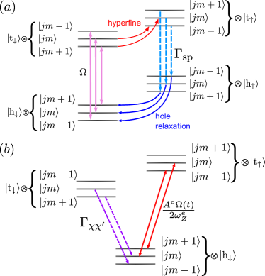
Figure 1: (a) Level scheme for electronic and nuclear states. The hyperfine sublevels are denoted with their total nuclear spin quantum numbers $j$ and $m$. The trion state $|\mathrm{t}_{\downarrow}\rangle$ with angular momentum (along $z$) $M=-1/2$ is pumped by the laser light with Rabi frequency $\Omega$ from the heavy hole state $|\mathrm{h}_{\downarrow}\rangle$ with $M=-3/2$. The hyperfine interaction couples the trion state $|\mathrm{t}_{\downarrow}\rangle$ and $|\mathrm{t}_{\uparrow}\rangle$ ($M=1/2$) and changes the $m$ quantum number of the nuclear system. The trion states can relax by spontaneous emission with the rate $\Gamma_{\mathrm{sp}}$. (b) Reduced level scheme with mechanisms for nuclear polarization in the trion - heavy hole system by spin-forbidden relaxation with rate $\Gamma_{\chi\chi^{\prime}}$ from $|\mathrm{t}_{\downarrow}\rangle$, or by spin-forbidden optical transitions between $|\mathrm{h}_{\downarrow}\rangle$ and $|\mathrm{t}_{\uparrow}\rangle$.

Here, the sum runs over all $N$ nuclei within the quantum dot. The operator $I_{z}^{k}$ describes the $z$ component of the $k$th nuclear spin. In Eq. (4), we have introduced the spin ladder operators defined as $S_{\pm}^{\mathrm{e}}=S_{x}^{\mathrm{e}}\pm\mathrm{i}S_{y}^{\mathrm{e}}$ and $I_{\pm}^{k}=I_{x}^{k}\pm\mathrm{i}I_{y}^{k}$. The hyperfine coupling constants with the $k$th nucleus are given by $A_{k}^{\mathrm{e}}=v_{k}^{\mathrm{e}}\nu_{0}\left|\psi^{\mathrm{e}}(\mbox{\boldmath$r$}_{k})\right|^{2}$ and $A_{k}^{\mathrm{h}}=v_{k}^{\mathrm{h}}\nu_{0}\left|\psi^{\mathrm{h}}(\mbox{\boldmath$r$}_{k})\right|^{2}$, where $v_{k}^{\mathrm{e}(\mathrm{h})}$ is the hyperfine coupling strength of the electron spin (heavy hole), $\nu_{0}$ the volume of a unit cell, and $\psi^{\mathrm{e}(\mathrm{h})}(\mbox{\boldmath$r$}_{k})$ is the envelope wave function of the electron (heavy hole).

The homogeneous approximation of the Hamiltonian (4) is performed by replacing the position-dependent coupling constant by $A^{\mathrm{e}}/N$, where $A^{\mathrm{e}}$ is the average hyperfine coupling constant (for InP quantum dots, $A^{\mathrm{e}}=110\,\mathrm{\mu eV}$ chekhovich_prl2010 ). The interaction strength between a heavy hole and the $k$th nuclear spin is given by $A_{k}^{\mathrm{h}}$. It differs from the electron hyperfine constant due to a different type of wave function. It was found theoretically and confirmed experimentally, that $A^{\mathrm{e}}\approx-0.11A^{\mathrm{e}}$ fischer_prb2008 ; chekhovich_prl2011 ; fallahi_prl2010 .

We omit the transverse terms of the effective heavy hole hyperfine interaction, which can contribute to nuclear spin polarization fischer_prb2008 . The coupling constants for the longitudinal and transverse hyperfine terms of the heavy hole are different due to the anisotropic character of the interaction. This leads to a transverse hyperfine coupling constant which is approximately two orders of magnitude smaller than the longitudinal one, $\left|A_{\perp}^{\mathrm{h}}\right|<0.06\left|A_{z}^{\mathrm{h}}\right|$ fischer_prb2008 . In addition, the large Zeeman energy ($B=2.5\,\mathrm{T}$) renders hyperfine assisted relaxation of heavy holes small compared to other physical mechanisms playing a role in the polarization of nuclear spins fras2012 .

In the following, we split the hyperfine Hamiltonian into longitudinal and transverse contributions. The longitudinal term,

$$H_{\mathrm{HF}}^{z}=\sum_{k=1}^{N}\left(A_{k}^{\mathrm{e}}S_{z}^{\mathrm{e}}I_{z}^{k}+A_{k}^{\mathrm{h}}S_{z}^{\mathrm{h}}I_{z}^{k}\right),$$ (5)

only produces a spin-dependent energy shift (Overhauser shift) of the electronic states, while the transverse part,

$$H_{\mathrm{HF}}^{\perp}=\frac{1}{2}\sum_{k=1}^{N}A_{k}^{\mathrm{e}}\left(S_{+}^{\mathrm{e}}I_{-}^{k}+S_{-}^{\mathrm{e}}I_{+}^{k}\right)$$ (6)

provides the mechanism for polarizing the nuclear spins by transferring magnetic moment from the electron spin to the nuclear spin ensemble.

The time dependence of Hamiltonian (1) can be removed by performing a canonical transformation,

$$H\to H^{\prime}={\rm e}^{\mathrm{i}\xi t/\hbar}(H-\xi){\rm e}^{-\mathrm{i}\xi t/\hbar}.$$ (7)

For our problem, we have

$$\xi=\left(E_{\mathrm{t}}-\frac{\hbar}{2}\omega_{Z}^{\mathrm{e}}-\frac{\hbar\Delta}{2}\right)\tau_{\mathrm{e}}-\hbar\left(\omega_{Z}^{\mathrm{h}}+\Delta\right)\tau_{\mathrm{h}},$$ (8)

where $\tau_{\mathrm{h}}=|\mathrm{h}_{\downarrow}\rangle\langle\mathrm{h}_{\downarrow}|+|\mathrm{h}_{\uparrow}\rangle\langle\mathrm{h}_{\uparrow}|$ is the projection operator onto the heavy-hole spin states. The detuning of the laser frequency from the heavy hole down to trion down, $|\mathrm{h}_{\downarrow}\rangle\rightarrow|\mathrm{t}_{\downarrow}\rangle$, transition energy is given by $\Delta=E_{\mathrm{t}}/\hbar+\tfrac{1}{2}(\omega_{Z}^{\mathrm{h}}-\omega_{Z}^{\mathrm{e}})-\omega_{\mathrm{L}}$. The transformation only acts non-trivially on $H_{0}$ [Eq. (2)], and $H_{\mathrm{L}}(t)$ [Eq. (3)]. We find

$$H_{0}\to H_{0}^{\prime}=\hbar\omega_{Z}^{\mathrm{e}}|\mathrm{t}_{\uparrow}\rangle\langle\mathrm{t}_{\uparrow}|+\frac{\hbar\Delta}{2}\tau_{\mathrm{e}}+\hbar\omega_{Z}^{\mathrm{h}}|\mathrm{h}_{\uparrow}\rangle\langle\mathrm{h}_{\uparrow}|-\frac{\hbar\Delta}{2}\tau_{\mathrm{h}},$$ (9)

and

$$H_{\mathrm{L}}(t)\to H_{\mathrm{L}}^{\prime}=\hbar\Omega\left(|\mathrm{t}_{\downarrow}\rangle\langle\mathrm{h}_{\downarrow}|+|\mathrm{h}_{\downarrow}\rangle\langle\mathrm{t}_{\downarrow}|\right),$$ (10)

after performing the rotating-wave approximation on $H_{\mathrm{L}}^{\prime}$.

The Hamiltonian defined in Eq. (1) becomes then,

$$H^{\prime}=H_{0}^{\prime}+H_{\rm L}^{\prime}+H_{\mathrm{HF}}^{z}+H_{\mathrm{HF}}^{\perp}.$$ (11)

We further eliminate the hyperfine spin-flip terms from Eq. (11) by applying a Schrieffer-Wolff transformation latta_nature2009 ; issler_prl2010 ; bravyi_annphys2011

$$H^{\prime}\to\tilde{H}=\mathrm{e}^{S}H^{\prime}\mathrm{e}^{-S}=\sum_{j=0}^{\infty}\frac{\left[S,H^{\prime}\right]^{(j)}}{j!},$$ (12)

where we have used the recursive definition

$$\left[S,H^{\prime}\right]^{(0)} =H^{\prime},$$ (13)

$$\left[S,H^{\prime}\right]^{(1)} =\left[S,H^{\prime}\right],$$

$$\left[S,H^{\prime}\right]^{(j)} =\left[S,\left[S,H^{\prime}\right]^{(j-1)}\right].$$

By applying the Schrieffer-Wolf transformation as defined in Eq. (12) with

$$S=\sum_{k=1}^{N}\frac{A_{k}^{\mathrm{e}}}{2\omega_{Z}^{\mathrm{e}}}\left(I_{-}^{k}|\mathrm{t}_{\uparrow}\rangle\langle\mathrm{t}_{\downarrow}|-I_{+}^{k}|\mathrm{t}_{\downarrow}\rangle\langle\mathrm{t}_{\uparrow}|\right),$$ (14)

we obtain an effective Hamiltonian with hyperfine interaction assisted spin-forbidden optical transitions:

$$\tilde{H}=H_{0}^{\prime}+H_{\rm L}^{\prime}+H_{\mathrm{HF}}^{z}+\sum_{k=1}^{N}\frac{\hbar A_{k}^{\mathrm{e}}\Omega}{2\omega_{Z}^{\mathrm{e}}}\left(I_{-}^{k}|\mathrm{t}_{\uparrow}\rangle\langle\mathrm{h}_{\downarrow}|+I_{+}^{k}|\mathrm{h}_{\downarrow}\rangle\langle\mathrm{t}_{\uparrow}|\right).$$ (15)

In the Hamiltonian (15), we only include terms of the Schrieffer-Wolff transformation up to the first order in $A^{\mathrm{e}}_{k}$. Higher-order terms describe, e.g., second order processes such as extrinsic nuclear-nuclear spin interactions assisted by two virtual electron spin flips yao_prb2006 ; latta_prl2011 ; klauser_2006 , which are of little interest here.

The effective Hamiltonian defined in Eq. (15) gives an intuitive picture of the optical pumping mechanism from heavy hole down to trion up [c.f. Fig. 1(b)]. When the laser frequency is on resonance with the transition $|\mathrm{h}_{\downarrow}\rangle\to|\mathrm{t}_{\uparrow}\rangle$, i.e., $\Delta=-\omega_{Z}^{\mathrm{e}}$, simultaneous absorption of a photon and transfer of angular momentum from the electron spin to the nuclear spin bath takes place. However, the coherent dynamics alone cannot explain the build-up of nuclear polarization. To correctly describe the pumping cycles, we need to include the spontaneous emission of the trion state. In this scenario, the quantum dot is initialized in the state $|\mathrm{h}_{\downarrow}\rangle$, optically pumped to the state $|\mathrm{t}_{\uparrow}\rangle$, simultaneously transferring the angular momentum of the electron spin to the nuclear bath, and the trion-up state decays by spontaneous emission to the state $|\mathrm{h}_{\uparrow}\rangle$ faster than it can be optically pumped back to $|\mathrm{h}_{\downarrow}\rangle$. The heavy hole up relaxes then via spin orbit to the initial heavy hole down climente2013 and another pumping cycle can start again. To describe the evolution of the system in presence of dissipation, we rely on the Lindblad master equation lindblad1976 ; breuer_petruccione .

III Lindblad Master Equation

The Lindblad master equation for the density matrix $\rho$ of the combined electronic and nuclear spin system is given by

$$\dot{\rho}=-\frac{\mathrm{i}}{\hbar}\left[\tilde{H},\rho\right]+\frac{1}{2}\sum_{j=1}^{d^{2}-1}\left(\left[L_{j}\rho,L_{j}^{{\dagger}}\right]+\left[L_{j},\rho L_{j}^{{\dagger}}\right]\right),$$ (16)

where the Lindblad operators $L_{j}$ describe different dissipation processes lindblad1976 ; breuer_petruccione , and $d$ is the dimension of the Hilbert space. Here, we only describe dissipative processes in the low-dimensional electronic system and therefore get by with a small number of Lindblad operators.

As mentioned earlier, a key dissipation process to explain the polarization dynamics is the spontaneous emission. Here, we take into account the spontaneous emission of a photon from the trion-down state to the corresponding hole state. This process is described by $L_{1}=\sqrt{\Gamma_{\mathrm{sp}}}|\mathrm{h}_{\downarrow}\rangle\langle\mathrm{t}_{\downarrow}|$, with $\Gamma_{\mathrm{sp}}=6\,\mathrm{GHz}$. In principle, there is a similar process for the other trion and hole states and a process that describes the relaxation of the heavy hole up to heavy hole down [cf. Fig. 1(a)]. However, since the heavy hole up does not play any major role in the polarization dynamics, we are going to consider a direct decay mechanism from the trion up to the heavy hole down, $L_{2}=\sqrt{\Gamma_{\mathrm{sp}}}|\mathrm{h}_{\downarrow}\rangle\langle\mathrm{t}_{\uparrow}|$. This is justified if the relaxation from heavy hole up to heavy hole down is not the bottleneck of the pumping cycle, i.e., the hole relaxation rate is considerably higher than the nuclear spin pumping rate. The latter has been demonstrated by Checkhovich et al. in Ref. [chekhovich_prl2010, ]. Thus, we assume a heavy-hole relaxation rate that fulfills $1/\Gamma_{\mathrm{sp}}+1/\Gamma_{\mathrm{h}_{\uparrow}\to\mathrm{h}_{\downarrow}}\approx 1/\Gamma_{\mathrm{sp}}$. Finally, we note that heavy-hole relaxation rates as short as $10\,\mathrm{ps}$ were reported in Ref. [climente2013, ]. This allows us to reduce the dimension of the electronic Hilbert subspace by omitting the heavy hole-up.

In addition to these two relaxation mechanisms, we include an additional process to describe the experimentally observed nuclear polarization when the laser frequency is on resonance with the transition $|\mathrm{h}_{\downarrow}\rangle\to|\mathrm{t}_{\downarrow}\rangle$, i.e. $\Delta=0$. The mechanism leading to polarization in this case is substantially different from what happens when $\Delta=-\omega_{Z}^{\mathrm{e}}$. The heavy hole down is optically excited to the trion-down state. At this point, there are two different relaxation paths: the trion down can either relax back to the heavy hole down by both spontaneous or stimulated emission or it can relax to the heavy hole up by transferring angular momentum to the nuclear bath. We describe the latter mechanism with the Lindblad operators, $L_{\chi\chi^{\prime}}=\sqrt{\Gamma_{\chi\chi^{\prime}}}|\mathrm{h}_{\uparrow}\,\chi\rangle\langle\mathrm{t}_{\downarrow}\,\chi^{\prime}|+\sqrt{\Gamma_{\mathrm{h}_{\uparrow}\to\mathrm{h}_{\downarrow}}}|\mathrm{h}_{\downarrow}\chi\rangle\langle\mathrm{h}_{\uparrow}\chi|$, where $\chi=j_{1}m_{1}\cdots j_{n}m_{n}$ labels collective angular momentum states of nuclear spins, which have been arranged into $n$ groups according to their hyperfine coupling strength $A_{i}^{\mathrm{e}}$ with the electronic spin. Since $\Gamma_{\mathrm{h}_{\uparrow}\to\mathrm{h}_{\downarrow}}\gg\Gamma_{\mathrm{sp}}$ and $\Gamma_{\chi\chi^{\prime}}\propto\Gamma_{\mathrm{sp}}$, we can approximate $L_{\chi\chi^{\prime}}$ to $L_{\chi\chi^{\prime}}\simeq\sqrt{\Gamma_{\chi\chi^{\prime}}}|\mathrm{h}_{\downarrow}\,\chi\rangle\langle\mathrm{t}_{\downarrow}\,\chi^{\prime}|$. The rates $\Gamma_{\chi\chi^{\prime}}$ are calculated in the following with help of Fermi’s golden rule.

III.1 Forbidden relaxation rate

We describe the interaction of the trion-heavy-hole system with the radiation field with Hamiltonian $H_{\rm rad}$. We have, in the dipole approximation scullyQO ,

$$H_{\mathrm{rad}}=-\mbox{\boldmath$d$}\cdot\mbox{\boldmath$E$},$$ (17)

where $d$ is the dipole operator of the quantum dot states and $E$ is the quantized electric field,

$$\mbox{\boldmath$E$}=\sum_{\mbox{\boldmath$\scriptstyle{k}$},\,\lambda}\sqrt{\frac{\hbar\omega_{k}}{2\varepsilon_{0}V}}\mbox{\boldmath$e$}_{\mbox{\boldmath$\scriptstyle{k}$},\,\lambda}\left(a^{\dagger}_{\mbox{\boldmath$\scriptstyle{k}$},\,\lambda}+a_{\mbox{\boldmath$\scriptstyle{k}$},\,\lambda}\right),$$ (18)

with $\varepsilon_{0}$ the vacuum permittivity. We have decomposed the field confined in a box of volume $V$ into Fourier modes with periodic boundary conditions. Each mode is associated with a wave vector $k$, two transverse polarization vectors $\mbox{\boldmath$e$}_{\mbox{\boldmath$\scriptstyle{k}$},\,\lambda}$, and frequency $\omega_{k}$. Furthermore, we have introduced the annihilation and creation operators $a_{\mbox{\boldmath$\scriptstyle{k}$},\,\lambda}$ and $a^{\dagger}_{\mbox{\boldmath$\scriptstyle{k}$},\,\lambda}$ of a photon with wave vector $k$ and polarization $\mbox{\boldmath$e$}_{\mbox{\boldmath$\scriptstyle{k}$},\,\lambda}$.

We will use $H_{\mathrm{rad}}$ as a perturbation and apply Fermi’s golden rule to compute the rate $\Gamma_{\chi\chi^{\prime}}$. In order to do so, we first need to find the eigenstates of $H_{0}+H_{\rm HF}^{z}+H_{\rm{HF}}^{\perp}$. This becomes particularly arduous due to the hyperfine interaction. To ease our task, we can instead use approximate eigenstates found with perturbation theory. This is possible thanks to the large Zeeman splitting of the electronic states.

We use $H_{0}+H_{\mathrm{HF}}^{z}$ as unperturbed Hamiltonian and $H_{\mathrm{HF}}^{\perp}$ as perturbation. The eigenstates of the unperturbed Hamiltonian can be written as $|\psi^{(0)}_{e\,\chi}\rangle=|e\,\chi\rangle$, where $|e\rangle$ labels trion and heavy hole states. Using first order perturbation theory, we find the corrections for the states $|\mathrm{h}_{\uparrow}\,\chi\rangle$ and $|\mathrm{t}_{\downarrow}\,\chi\rangle$, which respectively, read as

$$|\psi^{(1)}_{\mathrm{h}_{\uparrow}\,\chi}\rangle = 0;$$ (19)

$$|\psi^{(1)}_{\mathrm{t}_{\downarrow}\,\chi}\rangle = \frac{1}{2}\sum_{k}\frac{A^{\mathrm{e}}_{k}\sqrt{j_{k}(j_{k}+1)-m_{k}(m_{k}-1)}}{E^{(0)}_{\mathrm{t}_{\downarrow}\,\chi}-E^{(0)}_{\mathrm{t}_{\uparrow}\,\chi_{k}}}\times$$ (20)

$$|\mathrm{t}_{\uparrow}\,\chi_{k}\rangle,$$

with $\chi_{k}=j_{1}m_{1}\cdots j_{k}m_{k}-1\cdots j_{n}m_{n}$. Here $E^{(0)}_{\mathrm{t}_{\downarrow}\,\chi}=E_{\mathrm{t}}-\omega^{\mathrm{e}}_{\mathrm{Z}}/2-\sum_{i}A^{\mathrm{e}}_{i}m_{i}/2$ and $E^{(0)}_{\mathrm{t}_{\uparrow}\,\chi_{k}}=E_{\mathrm{t}}+\omega^{\mathrm{e}}_{\mathrm{Z}}/2+\sum_{i}A^{\mathrm{e}}_{i}m_{i}/2-A^{\mathrm{e}}_{k}/2$. The first-order correction to the energy is identically zero for all states, $E^{(1)}_{e\,\chi}=0$.

The transition rate $\Gamma_{\chi\chi^{\prime}}$ is then given by

$$\Gamma_{\chi\chi^{\prime}}=\frac{2\pi}{\hbar}\left|\langle\mathrm{f}|H_{\mathrm{rad}}|\mathrm{i}\rangle\right|^{2}\rho(E_{\mathrm{i}}-E_{\mathrm{f}}),$$ (21)

with $|\mathrm{f}\rangle=|\psi_{\mathrm{h}_{\uparrow}\,\chi^{\prime}},\,1\rangle$ and $|\mathrm{i}\rangle=|\psi_{\mathrm{t}_{\downarrow}\,\chi},\,0\rangle$. We denote the state of the radiation field by $|0\rangle$ (no photon) and $|1\rangle$ (one photon emitted). The energies of the initial and final state are $E_{\mathrm{i}}=E_{\mathrm{t}}-\omega^{\mathrm{e}}_{\mathrm{Z}}/2$ and $E_{\mathrm{f}}=\omega^{\mathrm{h}}_{\mathrm{Z}}/2+\omega_{\gamma}$, where $\omega_{\gamma}$ is the energy of the emitted photon.

The evaluation of Eq. (21) yields

$$\Gamma_{\chi\chi^{\prime}}=\frac{\Gamma_{\mathrm{sp}}}{4}\left|\sum_{k}\frac{A^{\mathrm{e}}_{k}\sqrt{j_{k}(j_{k}+1)-m_{k}(m_{k}-1)}}{\omega_{\mathrm{Z}}^{\mathrm{e}}+\sum_{l}A_{l}^{\mathrm{e}}m_{l}-\frac{A^{\mathrm{e}}_{k}}{2}}\right|^{2}\delta_{\chi,\chi^{\prime}_{k}},$$ (22)

where we have used scullyQO ; breuer_petruccione ,

$$\Gamma_{\mathrm{sp}}=\frac{2\pi}{\hbar}\left|\langle\mathrm{h}_{\uparrow}\,1|H_{\mathrm{rad}}|\mathrm{t}_{\uparrow}\,0\rangle\right|^{2}\rho(E_{\mathrm{i}}-E_{\mathrm{f}}),$$ (23)

with $\Gamma_{\mathrm{sp}}$ the spontaneous emission rate of the trion state.

We assume the spontaneous relaxation rate of the trion-up and -down states to be the same. The spontaneous emission follows a cubic dependence on the energy difference between the initial and final states, $\Gamma_{\mathrm{sp}}\propto\omega_{\mathrm{fi}}^{3}$. Having this in mind and noticing that both Zeeman splittings are four orders of magnitude smaller than the required energy to create a trion, $\hbar\omega^{\mathrm{e}(\mathrm{h})}_{\mathrm{Z}}/E_{\mathrm{t}}\simeq 10^{-4}$, it is perfectly reasonable to assume that both spontaneous emission rates are nearly identical.

Another process that could lead to nuclear spin polarization is hyperfine-mediated phonon spin flips. However, from the experimental data presented in Ref. [chekhovich_prl2010, ], there is no evidence that such processes play an important role in the dynamics. Both the absence of polaronic sidebands in the photoluminescence spectra of the quantum dot and the absence of side peaks in the measurement of the nuclear spin polarization seem to indicate very weak phonon coupling. One would indeed expect to see polarization side peaks (both sides of the main peak) if the emission or absorption of a phonon would assist the allowed (forbidden) transition when the laser frequency is detuned off resonance.

III.2 Solutions of the master equation

Since the Hamiltonian $\tilde{H}$ [Eq. (15)] is time independent, the master equation (16) is a system of homogeneous differential equations of first-order. Using a superoperator formalism, we can rewrite Eq. (16) as

$$\dot{\rho}(t)=\mathcal{L}\rho(t).$$ (24)

Interpreting the above equation as a vector equation, we can write the solution for $\rho(t)$ as

$$\rho(t)=\sum_{i}c_{i}\,\mbox{\boldmath$v$}_{i}\,e^{\lambda_{i}t},$$ (25)

where $\lambda$ and $v$ are the eigenvalues and eigenvectors of $\mathcal{L}$, respectively. The coefficients $c_{i}$ can be found from the initial conditions,

$$\rho(0)=\sum_{i}c_{i}\mbox{\boldmath$v$}_{i}.$$ (26)

For the initial conditions of the total density matrix we apply the sudden approximation coish_prb2004 . We assume that at times $t<0$, the electronic ($\rho_{\mathrm{e}}$) and nuclear ($\rho_{\mathrm{nuc}}$) density matrices are uncorrelated and for $t=0$ the state of the total system, $\rho$, is given by $\rho(0)=\rho_{\mathrm{e}}(0)\otimes\rho_{\mathrm{nuc}}(0)$. The initial state for the electronic system is,

$$\rho_{\mathrm{e}}(t=0)=|\mathrm{h}_{\downarrow}\rangle\langle\mathrm{h}_{\downarrow}|.$$ (27)

The initial nuclear state is assumed to be a fully mixed state. This assumption is justified by the fact that under normal experimental conditions the thermal energy is much larger than the nuclear Zeeman, $k_{\mathrm{B}}T\gg E_{\mathrm{Z}}^{\mathrm{nuc}}$. Thus, it is reasonable to assume a fully unpolarized nuclear state,

$$\rho_{\mathrm{nuc}}=\sum_{\chi}p(\chi)|\chi\rangle\langle\chi|.$$ (28)

By assuming the nuclear spins to be spin-$1/2$ and considering the case of a Dicke state $|jm\rangle$, we derive the probability distribution $p(\chi)$. Since we can write the probability for a Dicke state as the probability to find a given $j$ times the conditional probability of finding $m$ knowing $j$, $p(j,m)=p_{j}(j)p_{m}(m|j)$, our task is reduced to find the degeneracy $g(j)$ of the quantum number $j$. We have $p(j,m)=g(j)p_{m}(m|j)/\mathrm{dim}(\mathcal{H})$, where $\mathrm{dim}(\mathcal{H})=2^{N}$ is the total number of nuclear spin states. For a thermal state the distribution of $m$ for a given $j$ is uniform,

$$p_{m}(m|j)=\frac{[\Theta(j+m)-\Theta(j-m)]}{2j+1},$$ (29)

where $\Theta(x)$ is the Heaviside step function. The degeneracy $g(j)$ can be found following the method of Ref. [mandel_wolf, ], we find

$$g(j)=\frac{(2j+1)^{2}N!}{\left(\frac{N}{2}+j+1\right)!\left(\frac{N}{2}-j\right)!}.$$ (30)

As a simple and intuitive example consider the case of two spins ($N=2$). For this case, we can explicitly construct the four Dicke states $\{|0,0\rangle,|1,-1\rangle,|1,0\rangle,|1,1\rangle\}$, which are the well-known singlet ($j=0$) and triplet states ($j=1$). Equation (30) for $j=0$ and $1$ yields, respectively, $g(0)=1$ and $g(1)=3$. Combining the previously derived results, we arrive at

$$p(j,m)=\frac{(2j+1)N![\Theta(j+m)-\Theta(j-m)]}{\left(\frac{N}{2}+j+1\right)!\left(\frac{N}{2}-j\right)!2^{N}}.$$ (31)

This result is straightforwardly generalized for the case of a state $|\chi\rangle$,

$$p(\chi)=\prod_{i=1}^{n}p(j_{i},m_{i}),$$ (32)

with $N$ in Eq. (31) being replaced by $N_{i}$, i.e. the number of nuclear spins in group $i$. Finally, we arrive at the expression of the initial density matrix,

$$\rho(0)=\sum_{\chi}p(\chi)|\mathrm{h}_{\downarrow}\chi\rangle\langle\mathrm{h}_{\downarrow}\chi|.$$ (33)

IV Results

We calculate the nuclear spin polarization as a function of the pumping time $t_{\mathrm{pump}}$ and as a function of laser detuning $\Delta$ for a fixed pumping time. The polarization $P$ is calculated according to

$$P(t)=\sum_{k}A_{k}^{\mathrm{e}}\langle I^{z}_{k}(t)\rangle,$$ (34)

with $\langle I^{z}_{k}(t)\rangle=\mathrm{Tr}\,[I^{z}_{k}\rho_{\mathrm{nuc}}(t)]$ and $\rho_{\mathrm{nuc}}(t)=\mathrm{Tr}_{\rm e}[\rho(t)]$ is obtained by taking the partial trace over the electronic states. This definition corresponds to the experimental procedure that is employed to measure the nuclear spin magnetization, which is done by measuring the shift of the electronic Zeeman splitting and interpreting it as an effective magnetic field, $B_{\mathrm{nuc}}=\sum_{k}A_{k}^{\rm e}\langle I_{k}^{z}\rangle/g^{*}\mu_{\mathrm{B}}$.

IV.1 Homogeneous hyperfine coupling

The simplest way to solve Eq. (24) is to assume a homogeneous hyperfine coupling constant, $A_{k}^{\mathrm{e}}=A^{\mathrm{e}}/N$ ($A^{\mathrm{e}}=110\,\mathrm{\mu eV}$ for InP quantum dots chekhovich_prl2010 ). This model corresponds to the case in which the electronic envelope wave function in the quantum dot is a plane wave. It is often referred to as “box” model kozlov_arxiv2008 ; petrov_prb2009 . In this case, a state $|\chi\rangle$ reduces to a Dicke state $|jm\rangle$. In this basis, the density matrix is block-diagonal (each block corresponding to a fixed $j$), which allows us to compute the time evolution separately for each block. This is a direct consequence of the lack of transitions between different $j$ states.

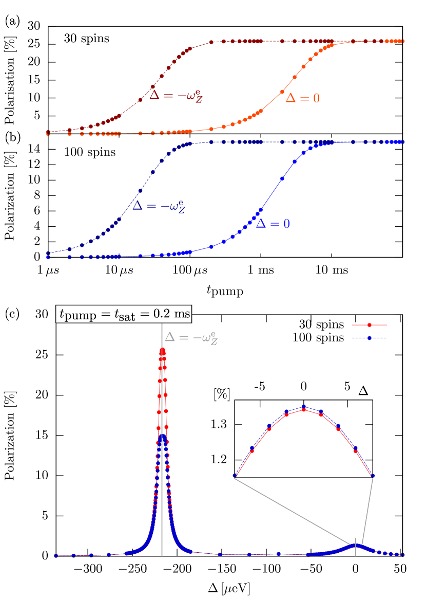
Figure 2: Nuclear spin polarization calculated for the case of homogeneous hyperfine coupling constant. (a) Saturation of the polarization for $N=30$ by pumping the spin-forbidden transition at a laser detuning $\Delta=-\omega_{\mathrm{Z}}^{\mathrm{e}}=-220\,\mathrm{\mu eV}$ and the allowed transition at $\Delta=0$. (b) Same as (a), but with $N=100$. (c) The degree of nuclear polarization for $N=30$ and $N=100$ after a pumping time $t_{\mathrm{pump}}=0.2\,\mathrm{ms}$ as function of laser detuning $\Delta$. The maximal degree of polarization observed for $\Delta=-\omega_{\mathrm{Z}}^{\mathrm{e}}$ reduces for increasing number of spins. The vertical lines at $\Delta=-\omega_{Z}^{\mathrm{e}}$ and $\Delta=0$ are visual guides to emphasize laser dragging effects and the change of optical resonance. Inset: magnification around $\Delta=0$ showing a difference in the polarization degree between $N=30$ and $100$.

In Fig. 2, we present results for the polarization as a function of pumping time, $t_{\mathrm{pump}}$, and laser detuning, $\Delta$, for different number of spins. In order to find a percentage, we have divided $P$ by the maximally achievable polarization, $P_{\mathrm{max}}=-N/2$. Here, the minus sign reflects the direction nuclear spins are polarized with the present pumping mechanism. In accordance with the experimental findings chekhovich_prl2010 , we observe a build up of polarization for $\Delta=0$ and $-\omega_{\mathrm{Z}}^{\mathrm{e}}$, but not to the same extent [c.f. Fig. 2(c)]. Moreover, we observe a decline of the possible maximal degree of polarization with increasing number of nuclear spins.

The fact that a polarization of 100% is not possible for homogeneous hyperfine coupling is attributed to the formation of a hyperfine dark state imamoglu_prl2003 ; christ_prb2007 ; kozlov_JETP2007 ; ribeiro_2009 ,

$$\rho_{\mathrm{nuc}}(t\geq t_{\mathrm{sat}})=\sum_{j}p_{j}(j)|j-j\rangle\langle j-j|.$$ (35)

The population of this state cannot be changed by the hyperfine interaction, since there is no population transfer between different $j$ blocks.

The polarization of such a state can be straightforwardly evaluated by using $p_{j}(j)=g(j)/2^{N}$. We have

$$P^{N}_{\mathrm{sat}}=\frac{1}{P_{\mathrm{max}}}\sum_{j}^{\frac{N}{2}}j\,p_{j}(j),$$ (36)

where the lower bound of the sum is $j=0$ for even $N$ and $j=1/2$ for an odd $N$. The sum (36) can be evaluated analytically:

$$P_{\rm sat}^{N}=-\frac{1}{N}+\left\{\begin{array}[]{l}\frac{2(1+2N)\Gamma\left(\frac{N+1}{2}\right)}{\sqrt{\pi}N^{2}\Gamma\left(\frac{N}{2}\right)},\quad N\>\mathrm{even},\\ \frac{2\Gamma\left(\frac{N}{2}\right)}{\sqrt{\pi}\Gamma\left(\frac{N+1}{2}\right)},\quad N\>\mathrm{odd}.\end{array}\right.$$ (37)

Using Sterling’s formula, we find that both expressions asymptotically approach $P^{N}\approx\sqrt{\pi/8N}$.

The evaluation of Eq. (37) for $N=30$ and $100$ respectively yields, $P^{30}_{\mathrm{sat}}\simeq 26.04\%$ and $P^{100}_{\mathrm{sat}}\simeq 14.99\%$ in a very good agreement with our results. The asymptotic behavior can be easily understood by considering the distribution $p_{j}(j)$ for increasing number of spins (cf. Fig. 3). For systems with a large number of nuclear spins, the distribution only has sizable values around a small vicinity of its maximum ($j\simeq\sqrt{N/2}$). This results in the values of $j$ that could potentially lead to high polarization, such as $j=N/2$, to play no role in the average polarization since $p_{j}(N/2)_{N\gg 1}\sim 0$. As an example, we have $P^{10^{4}}_{\mathrm{sat}}\sim 1\%$, with similar estimations found in Refs. [kozlov_JETP2007, ] and [christ_prb2007, ]. This behavior for a large number of nuclear spins is far from experimentally observable values, therefore a model with homogeneous hyperfine coupling cannot be used for explaining the limit of the nuclear polarization observed in the experiments.

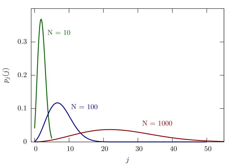
Figure 3: Distribution $p_{j}(j)$ of the total angular momentum $j$. The larger the system gets, the smaller the value of $p_{j}$ becomes for the most likely $j\sim\sqrt{N/2}$ and the faster it converges to $0$.

We have however to point out that such a model qualitatively reproduces all physical phenomena observed experimentally. In addition to the already discussed similarities with experimental data, it also reproduces dragging effects arising from the build-up of nuclear polarization. They can be noticed in Fig. 2(c), but are not prominent, because of two reasons: we can only model a small number of nuclear spins and achieve low degrees of polarization. Both of these facts correspond to negligible Overhauser fields compared to the electron Zeeman splitting. The build-up of the Overhauser field causes the laser dragging latta_nature2009 ; chekhovich_prl2010 and changes the optical resonance conditions. This leads to the maximal polarization to be shifted from the expected values of detuning, $\Delta=0$ and $\Delta=-\omega_{\mathrm{Z}}^{\mathrm{e}}$.

IV.2 Inhomogeneous hyperfine coupling

In a more realistic model for the hyperfine interaction, an electron spin in a quantum dot couples to nuclear spins at different lattice sites with different strengths [c.f. Eqs. (5) and (6)]. In the case where the confinement is assumed to be harmonic, we have $A_{k}^{\mathrm{e}}=A_{0}^{\mathrm{e}}\exp(-r_{k}^{2}/r_{0}^{2})$ coish_prb2004 ; tsyplyatyev_prl2011 , where $r_{0}$ is the radial size of the confinement. $A^{\mathrm{e}}_{1}$ is the coupling strength of the nuclear spin in the center of the quantum dot and $r_{k}$ is the radius of the $k$th shell with a constant coupling. With nuclear spins divided in many groups of constant coupling, the problem becomes more complex, but we can still use the same concepts as for the homogeneous coupling case. In the latter case, the quantum number $j$ is conserved and in the former case the conserved quantum numbers are the total angular momenta of different groups: $j_{1},j_{2},\cdots,j_{n}$. Consequently, the nuclear density matrix is block diagonal for different sets of $j_{1},j_{2},\cdots,j_{n}$, and we can once more evaluate the nuclear dynamics separately for these blocks. Since the power of conventional computers does not allow us to compute the polarization dynamics for many groups of spins, we consider the case of two and three groups.

In Fig. 4 we present results for the nuclear polarization dynamics for two different coupling constants. As previously, we consider a different number of spins and compute the polarization as a function of pumping time, $t_{\mathrm{pump}}$, and detuning, $\Delta$. The results present a similar behavior as for the case of homogeneous hyperfine coupling (cf. Fig. 2). However, quantitatively there is a difference between the reachable maximal polarizations. The saturation of the polarization for $N_{1}=6$, $A_{1}^{\mathrm{e}}=10^{7}\,\mathrm{Hz}$ and $N_{2}=4$, $A_{2}^{\mathrm{e}}=10^{5}\,\mathrm{Hz}$ is $59\%$, it would be $42\%$ if the same number of spins were homogeneously coupled. For $N_{1}=4$ and $N_{2}=2$, we find $74.7\%$, while it would have been $51\%$ for six homogeneously coupled spins.

As for the homogeneous case, the nuclear state is driven into a dark state for the hyperfine coupling, which is a generalization of Eq. (35):

$$\rho_{\mathrm{nuc}}(t\leq t_{\mathrm{sat}})=$$

$$\sum_{j_{1},\cdots,j_{n}}p_{\chi_{j}}(j_{1},\cdots,j_{n})\bigotimes_{i=1}^{n}|j_{i},-j_{i}\rangle\langle j_{i},-j_{i}|,$$ (38)

with $p_{\chi_{j}}(j_{1},\cdots,j_{n})=\prod_{i=1}^{n}g(j_{i})/2^{N_{i}}$. We verify that this is indeed the case by computing the degree of polarization of the nuclear state given in Eq. (38). The generalization of Eq. (36) yields,

$$P_{\mathrm{sat}}^{\{N_{i}\}_{1}^{n}}=\frac{\displaystyle\sum_{j_{1}\cdots j_{n}}^{N_{1}/2\cdots N_{n}/2}(A_{1}^{\mathrm{e}}j_{1}+\cdots+A_{n}^{\mathrm{e}}j_{n})p_{\chi_{j}}(j_{1},\cdots,j_{n})}{\displaystyle\sum_{k=1}^{n}A_{k}^{\mathrm{e}}\frac{N_{k}}{2}}.$$ (39)

Using Eq. (39) we find for $N_{1}=6$ and $N_{2}=4$, $P_{\mathrm{sat}}^{6,4}=59.25\%$ and for $N_{1}=4$ and $N_{2}=2$, $P_{\mathrm{sat}}^{6,4}=74.69\%$ in very good agreement with our results.

To confirm our observations, we have also computed the saturation of the polarization for $n=3$. The total number of spins was kept constant, while the number of spins in the groups was varied. We have chosen $A^{\mathrm{e}}_{1}=10^{8}\,\mathrm{Hz}$, $A^{\mathrm{e}}_{2}=10^{7}\,\mathrm{Hz}$, and $A^{\mathrm{e}}_{3}=10^{6}\,\mathrm{Hz}$. The results are presented in Fig. 5.

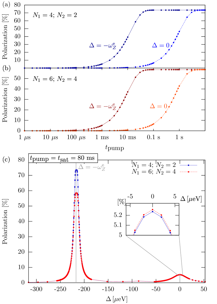
Figure 4: Nuclear polarization calculated for inhomogeneous hyperfine interaction. Due to the limitation of the computing power at our disposal, we have simulated two groups of nuclear spins with coupling strengths $A^{\mathrm{e}}_{1}=10^{7}$ Hz and $A^{\mathrm{e}}_{2}=10^{5}$ Hz: the saturation of the polarization for the laser detuning at the forbidden ($\Delta=-\omega_{\mathrm{Z}}^{\mathrm{e}}$) and allowed ($\Delta=0$) transitions for (a) $N_{1}=4,N_{2}=2$ and (b) $N_{1}=6,N_{2}=4$. (c) Nuclear polarization for different laser detunings and for different number of spins divided into two groups for $t_{\mathrm{pump}}=0.08\,\mathrm{s}$. The vertical lines at $\Delta=-\omega_{\mathrm{Z}}^{\mathrm{e}}$ and $\Delta=0$ are visual guides to emphasize the shift of the optical resonance.

We compare the polarization at saturation as obtained with the solution of the master equation and calculated using Eq. (39). We find very good agreement between both results, which indicates that the nuclear spin state is driven to the dark state described by Eq. (38). We have found $P_{\mathrm{sat}}^{4,2,2}=60\%$, $P_{\mathrm{sat}}^{2,4,2}=72\%$, and $P_{\mathrm{sat}}^{2,2,4}=74.7\%$.

As our results demonstrate, a more realistic treatment of the hyperfine interaction leads to a substantial increase in the maximal degree of nuclear polarization. Moreover, the results presented in Fig. 5 suggest that the polarization degree depends strongly on the group configurations, i.e., the number of spins per group, strength of the coupling (electronic envelope wave function), and (to a minor extent) on the total number of spins. Since Eq. (39) predicts accurately the degree of polarization, we can apply it for finding the maximal degree of nuclear polarizations for larger systems, mimicking to some extent the nuclear spins in quantum dots.

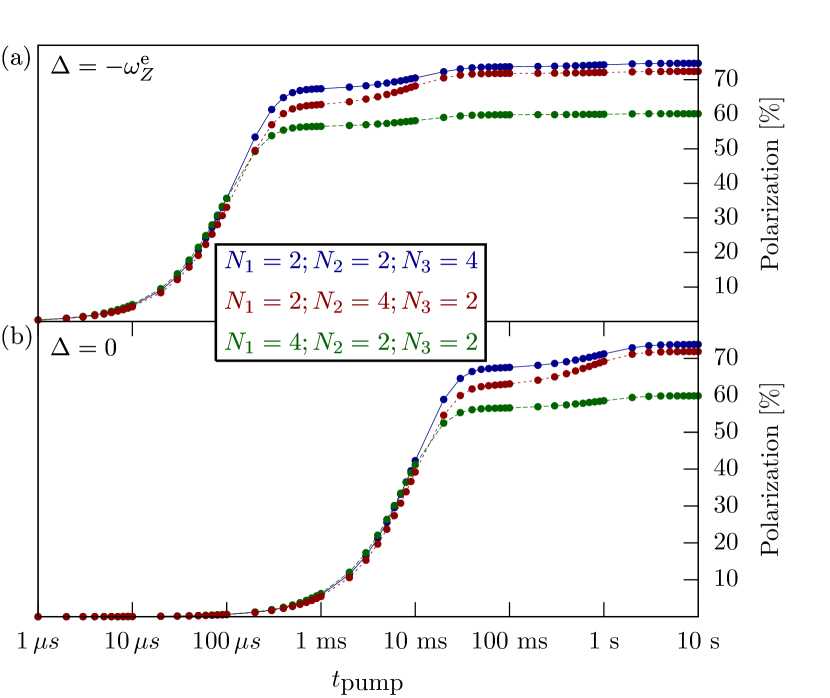
Figure 5: Saturation of nuclear polarization calculated for nuclear spins divided into three groups and inhomogeneously coupled to the electronic spin. The coupling strengths are $A^{\mathrm{e}}_{1}=10^{8}$ Hz, $A^{\mathrm{e}}_{2}=10^{7}$ Hz and $A^{\mathrm{e}}_{3}=10^{6}$ Hz. (a) Polarization at $\Delta=-\omega_{Z}^{\mathrm{e}}$; and (b) at $\Delta=0$.

For a more realistic description, we assumed a system where nuclear spins form a three-dimensional cubic lattice (InP has a zincblende lattice) and split the lattice sites into equidistant shells from the maximum of the electron wave function, which is assumed to have a Gaussian distribution. For a system of $360$ spins we obtained 25.5% of polarization and for $365$ spins 30.4%. The difference between the two cases comes from the relative position of the maximum of the electron wave function relative to the lattice: in the first case, it was set in the middle of the unit cell, and in the second case, it was exactly at a lattice site. This result clearly indicates that there is no universal value for $P_{\mathrm{sat}}$, but rather that every quantum dot has a different saturation polarization. We consider now a quantum dot made out of two elements (two sublattices) with different hyperfine coupling constants. We have to group the nuclear spins not only by considering the distance to the center, but also by taking into account the different hyperfine couplings of each species. If we consider the previous cases, but we divide the lattice into two sublattices, the degree of nuclear spin polarization of the dark state becomes 34.4% and 40.6%, respectively. This calculation shows that in realistic quantum dots, which consist of two and very often more elements, the achievable degree of polarization is higher than the one calculated with identical nuclear spins. We show in Appendices A and B the explicit distribution of $A_{k}$’s and $N_{k}$’s for both considered cases.

In our calculations, we have considered systems consisting of nuclear spins with $I=1/2$, whereas the relevant optically active semiconductor quantum dots are built up by materials (e.g., In and P) with $I\geq 1/2$. We can therefore raise the question if some of the neglected interactions could significantly affect the nuclear spin pumping. In our model, we have neglected nuclear-nuclear spin interactions, i.e., nuclear Zeeman energy, dipole-dipole coupling, and quadrupole splittings, the latter only being relevant for $I>1/2$. Among these, nuclear dipole-dipole interaction constitutes a competing mechanism that could prevent the formation of the dark state. However, experimental findings indicate that nuclear spin diffusion happens on time scales ranging from seconds to hours coish_statsolidi2009 ; tartakovskiiprivate . This indicates a small dipole coupling that can be neglected in comparison with the hyperfine-mediated nuclear dipole-dipole coupling, and which is the main source of diffusion during the pumping cycle. The effect of the nuclear Zeeman and quadrupole splitting is more subtle. The obvious change concerns Eq. (22), where the denominator would also include the difference in nuclear Zeeman energy and quadrupole splitting between the nuclear states $|\chi\rangle$ and $|\chi^{\prime}\rangle$. These are small corrections in comparison with the electron Zeeman energy and therefore they do not alter Eq. (22) significantly. However, when considering different isotopes, the nuclear Zeeman and quadrupole interactions force an additional division of nuclear spins with the same distance from the maximum of the electron wave function. Different isotopes have different nuclear gyromagnetic ratios and quadrupolar splittings which lead to slightly different forbidden relaxation rates. Such additional fragmentation leads to an increase of the maximal degree of polarization. A smaller number of nuclear spins per shell leads to an increase of the statistical weight of the states contributing the most to the degree of polarization (cf. Fig. 3).

V Conclusions

We have developed a master-equation formalism that allows us to partially explain recent experimental observations chekhovich_prl2011 on the saturation of the nuclear spin polarization when pumped via an optically spin-forbidden transition between a heavy hole and a trion state. We have identified both mechanisms leading to spin polarization depending on the laser detuning and we have found flip-flop rates that depend explicitly on the nuclear state.

Based on our formalism, we have calculated the exact time evolution of the nuclear spin polarization. Considering the nuclear spin bath as an ensemble of quantum spins, which is initially in thermal equilibrium, we have investigated two possible models for the hyperfine interaction: homogeneous and inhomogeneous. In both cases, the saturation of the nuclear polarization is attributed to the conservation of the total angular momentum of the whole nuclear state in the homogeneous case or of the particular groups of same coupling for the inhomogeneous case. In the latter, the degree of maximal nuclear polarization is consistent with the experimentally observed values. Our findings show that variations in the maximal degree of polarization depend on the chemical composition of the quantum dot and the distribution of the electron wave function inside of the quantum dot. However, the latter property offers a possible way to overcome the limit set by the dark state. It is possible to change the functional form of the electronic wave function by applying electric fields imamoglu_prl2003 ; christ_prb2007 . This would lead to a redefinition of the nuclear spin groups with the same hyperfine coupling constant, which would further allow hyperfine-mediated nuclear spin pumping. It has still to be proven experimentally that such a protocol can indeed achieve higher degrees of nuclear spin polarization than the one set by a dark state.

VI Acknowledgments

We acknowledge funding from the DFG within SFB 767 and SPP 1285 and from BMBF under the program QuaHL-Rep. H. R. also acknowledges funding from the Swiss NF.

Appendix A $A_{k}$ and $N_{k}$ distributions for a system of $360$ nuclear spins

In Fig. A.1, we present the strength of the hyperfine coupling constants $A_{k}$ [Fig. A.1(a)] and the number of nuclear spins $N_{k}$ [Fig. A.1(b)] as a function of the distance to the maximum of the wave function for a system made of identical nuclear spins. The distance is measured in units of the lattice constant $\rm{a}$. We note that the maximum of the wave function is not situated at a lattice site. For a three-dimensional cubic lattice, the $360$ nuclear spins are divided among 10 groups.

In Fig. A.1(c), we show the distribution of $A_{k}^{s}$ and in Fig. A.1(d) the number of nuclear spins $N_{k}^{s}$ ($s=\rm{A,\,B}$) for a system with two nuclear species. The nuclear spins of each species form a sublattice denoted $\rm{A}$ and $\rm{B}$. We have assumed for simplicity that each sublattice is constituted by the same number of nuclear spins.

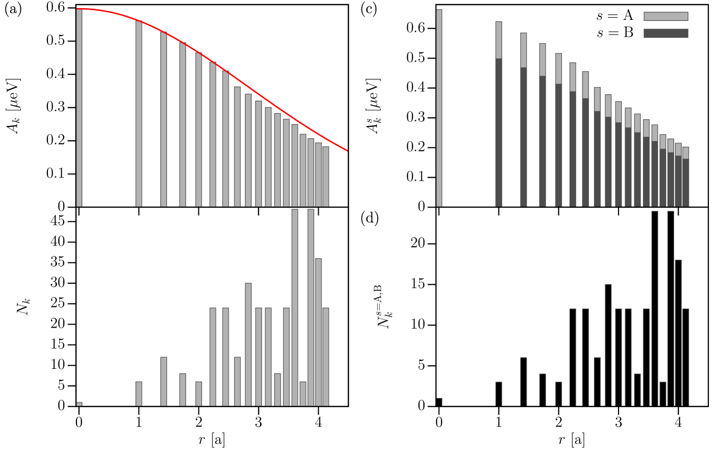
Figure A.1: (a) Hyperfine coupling constants $A_{k}$ and (b) number of nuclear spins $N_{k}$ as a function of the distance to the maximum of the wave function. The distance is given in units of the lattice constant $\rm{a}$. We have plotted in red the continuous distribution of hyperfine coupling constants $A(\mbox{\boldmath$r$})=A_{0}\exp[-(r/r_{0})^{2}]$. (c) Same as (a) for two sublattices $s=\rm{A,\,B}$. We denote the hyperfine coupling constant by $A_{k}^{s}$. (d) Number of nuclear spins $N_{k}^{s}$ in each sublattice.

Appendix B $A_{k}$ and $N_{k}$ distribution for a system of $365$ nuclear spins

In Fig. A.2, we present the same data as in the previous appendix, but for the maximum of the wave function situated at a lattice site.

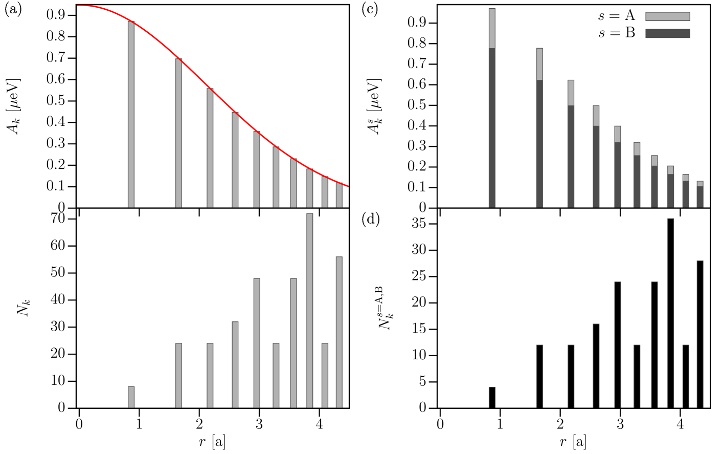
Figure A.2: (a) Hyperfine coupling constants $A_{k}$ and (b) number of nuclear spins $N_{k}$ as a function of the distance to the maximum of the wave function, which is located at a lattice site. The distance is measured in units of the lattice constant $\rm{a}$. The continuous distribution of hyperfine coupling constants, $A(\mbox{\boldmath$r$})=A_{0}\exp[-(r/r_{0})^{2}]$, is shown in red. (c) Same as (a) for a system made of two nuclear species divided into two sublattices ($s=\rm{A,\,B}$). (d) Number of nuclear spins $N_{k}^{s}$ for $s=\rm{A,\,B}$.

References

- (1) K. Ono, D. G. Austing, Y. Tokura, and S. Tarucha, Science 297, 1313 (2002).
- (2) J. R. Petta, A. C. Johnson, J. M. Taylor, E. A. Laird, A. Yacoby, M. D. Lukin, C. M. Marcus, M. P. Hanson, and A. C. Gossard, Science 309, 2180 (2005).
- (3) F. H. L. Koppens, C. Buizert, K. J. Tielrooij, I. T. Vink, K. C. Nowack, T. Meunier, L. P. Kouwenhoven, and L. M. K. Vandersypen, Nature 442, 766 (2006).
- (4) K. C. Nowack, F. H. L. Koppens, Yu. V. Nazarov, and L. M. K. Vandersypen, Science 318, 1430 (2007).
- (5) J. R. Petta, H. Lu, and A. C. Gossard, Science 327, 669 (2010).
- (6) H. Ribeiro, G. Burkard, J. R. Petta, H. Lu, and A. C. Gossard, Phys. Rev. Lett. 110, 086804 (2013).
- (7) C. Kloeffel and D. Loss, Annu. Rev. Condens. Matter Phys. 4, 51 (2013).
- (8) D. Loss and D. P. DiVincenzo, Phys. Rev. A 57, 120 (1998).
- (9) L. Chirolli and G. Burkard, Adv. In Phys. 57, 225 (2008).
- (10) W. A. Coish and J. Baugh, Phys. Stat. Solidi (b) 246, 2203 (2009).
- (11) A. V. Khaetskii, D. Loss, and L. Glazman, Phys. Rev. Lett. 88, 186802 (2002).
- (12) I. A. Merkulov, Al. L. Efros, and M. Rosen, Phys. Rev. B 65, 205309 (2002).
- (13) E. L. Hahn, Phys. Rev. 80, 580 (1950).
- (14) H. Y. Carr and E. M. Purcell, Phys. Rev. 94, 630 (1954).
- (15) W. A. Coish and D. Loss, Phys. Rev. B 70, 195340 (2004).
- (16) W. A. Coish and D. Loss, Phys. Rev. B 72, 125337 (2005).
- (17) X. Xu, W. Yao, B. Sun, D. G. Steel, A. S. Bracker, D. Gammon, and L. J. Sham, Nature 459, 1105 (2009).
- (18) A. Greilich, S. E. Economou, S. Spatzek, D. R. Yakovlev, D. Reuter, A. D. Wieck, T. L. Reinecke, and M. Bayer, Nat. Phys. 5, 262 (2009).
- (19) S. M. Clark, K.-M. C. Fu, Q. Zhang, T. D. Ladd, C. Stanley, and Y. Yamamoto, Phys. Rev. Lett. 102, 247601 (2009).
- (20) D. Press, K. De Greve, P. L. McMahon, T. D. Ladd, B. Friess, C. Schneider, M. Kamp, Sven Höfling, A. Forchel, and Y. Yamamoto, Nat. Phot. 4, 367 (2010).
- (21) W. M. Witzel and S. Das Sarma, Phys. Rev. B 74, 035322 (2006).
- (22) H. Bluhm, S. Foletti, I. Neder, M. Rudner, D. Mahalu, V. Umansky, and A. Yacoby, Nat. Phys. 7, 109 (2011).
- (23) J. M. Taylor, A. Imamoğlu, and M. D. Lukin, Phys. Rev. Lett. 91, 246802 (2003).
- (24) H. Schwager, J. I. Cirac, and G. Giedke, Phys. Rev. B 81, 045309 (2010).
- (25) P. Maletinsky, A. Badolato, and A. Imamoğlu, Phys. Rev. Lett. 99, 056804 (2007).
- (26) A. E. Nikolaenko, E. A. Chekhovich, M. N. Makhonin, I. W. Drouzas, A. B. Van’kov, J. Skiba-Szymanska, M. S. Skolnick, P. Senellart, D. Martrou, A. Lemaître, and A. I. Tartakovskii, Phys. Rev. B 79, 081303(R) (2009).
- (27) D. Gammon, S. W. Brown, E. S. Snow, T. A. Kennedy, D. S. Katzer, and D. Park, Science 277, 85 (1997).
- (28) S. G. Carter, A. Shabaev, S. E. Economou, T. A. Kennedy, A. S. Bracker, and T. L. Reinecke, Phys. Rev. Lett. 102, 167403 (2009).
- (29) M. N. Makhonin, K. V. Kavokin, P. Senellart, A. Lemaître, A. J. Ramsay, M. S. Skolnick, and A. I. Tartakovskii, Nat. Mat. 10, 844 (2011).
- (30) C. Latta, A. Högele, Y. Zhao, A. N. Vamivakas, P. Maletinsky, M. Kroner, J. Dreiser, I. Carusotto, A. Badolato, D. Schuh, W. Wegscheider, M. Atatüre, and A. Imamoğlu, Nature Phys. 5, 758 (2009).
- (31) A. I. Tartakovskii, T. Wright, A. Russell, V. I. Fal’ko, A. B. Van’kov, J. Skiba-Szymanska, I. Drouzas, R. S. Kolodka, M. S. Skolnick, P. W. Fry, A. Tahraoui, H.-Y. Liu, and M. Hopkinson, Phys. Rev. Lett. 98, 026806 (2007).
- (32) M. N. Makhonin, E. A. Chekhovich, P. Senellart, A. Lemaître, M. S. Skolnick, and A. I. Tartakovskii Phys. Rev. B 82, 161309(R) (2010).
- (33) E. A. Chekhovich, M. N. Makhonin, K. V. Kavokin, A. B. Krysa, M. S. Skolnick, and A. I. Tartakovskii, Phys. Rev. Lett. 104, 066804 (2010).
- (34) O. Tsyplyatyev and D. Loss, Phys. Rev. Lett. 106, 106803 (2011).
- (35) J. Fischer, W. A. Coish, D. V. Bulaev, and D. Loss, Phys Rev. B 78, 155329 (2008).
- (36) E. A. Chekhovich, A. B. Krysa, M. S. Skolnick, and A. I. Tartakovskii, Phys. Rev. Lett. 106, 027402 (2011).
- (37) P. Fallahi, S. T. Yilmaz, and A. Imamoğlu, Phys. Rev. Lett. 105, 257402 (2010).
- (38) F. Fras, B. Eble, P. Desfonds, F. Bernardot, C. Testelin, M. Chamarro, A. Miard, and A. Lemaître, Phys. Rev. B 86, 045306 (2012).
- (39) M. Issler, E. M. Kessler, G. Giedke, S. Yelin, I. Cirac, M. D. Lukin, and A. Imamoğlu, Phys. Rev. Lett. 105, 267202 (2010).
- (40) S. Bravyi, D. DiVincenzo, and D. Loss, Ann. Phys. 326, 2793 (2011).
- (41) W. Yao, R.-B. Liu, and L. J. Sham, Phys. Rev. B 74, 195301 (2006).
- (42) C. Latta, A. Srivastava, and A. Imamoğlu, Phys. Rev. Lett. 107, 167401 (2011).
- (43) D. Klauser, W. A. Coish, and D. Loss, Phys. Rev. B 73, 205302 (2006).
- (44) J. I. Climente, C. Segarra, and J. Planelles, New J. Phys. 15 093009 (2013).
- (45) G. Lindblad, Commun. Math. Phys. 48, 119 (1976).
- (46) H.-P. Breuer and F. Petruccione, The theory of open quantum systems, Oxford University Press, USA (2002).
- (47) M. O. Scullay and M. S. Zubairy, Quantum Optics, Cambridge University Press, U.K. (1997).
- (48) L. Mandel and E. Wolf, Optical coherence and quantum optics, Cambridge University Press, USA (1995).
- (49) G. G. Kozlov, arXiv:0801.1391, unpublished.
- (50) M. Yu. Petrov, G. G. Kozlov, I. V. Ignatiev, R. V. Cherbunin, D. R. Yakovlev, and M. Bayer, Phys. Rev. B 80, 125318 (2009).
- (51) A. Imamoğlu, E. Knill, L. Tian, and P. Zoller, Phys. Rev. Lett. 91, 017402 (2003).
- (52) G. G. Kozlov, JETP 105, 803 (2007).
- (53) H. Christ, J. I. Cirac, and G. Giedke, Phys. Rev. B 75, 155324 (2007).
- (54) H. Ribeiro and G. Burkard, Phys. Rev. Lett. 102, 216802 (2009).
- (55) In a private communication with A. Tartakovskii about the experiment presented in Ref. chekhovich_prl2010, , spin diffusion was measured to happen on a timescale on the order of the hour, i.e. two orders of magnitude longer that the total time required to reach saturation.