Thermal field theories and shifted boundary conditions

Abstract:

The analytic continuation to an imaginary velocity of the canonical partition function of a thermal system expressed in a moving frame has a natural implementation in the Euclidean path-integral formulation in terms of shifted boundary conditions. The Poincaré invariance underlying a relativistic theory implies a dependence of the free-energy on the compact length $L_{0}$ and the shift ${\bm{\xi}}$ only through the combination $\beta=L_{0}(1+{\bm{\xi}}^{2})^{1/2}$. This in turn implies that the energy and the momentum distributions of the thermal theory are related, a fact which is encoded in a set of Ward identities among the correlators of the energy-momentum tensor. The latter have interesting applications in lattice field theory: they offer novel ways to compute thermodynamic potentials, and a set of identities to renormalize non-perturbatively the energy-momentum tensor. At fixed bare parameters the shifted boundary conditions also provide a simple method to vary the temperature in much smaller steps than with the standard procedure.

1 Introduction

A relativistic thermal field theory can be formulated in the Euclidean path integral formalism by imposing on the fields periodic boundary conditions in the compact direction up to a shift ${\bm{\xi}}$ in the spatial directions [1, 2, 3]

$$\phi(L_{0},\bm{x})=\phi(0,\bm{x}-L_{0}\,\bm{\xi})\;.$$ (1)

The free-energy density can be defined as usual

$$f(L_{0},\bm{\xi})=-\frac{1}{L_{0}V}\ln Z(L_{0},\bm{\xi})\;,$$ (2)

where $Z(L_{0},\bm{\xi})$ is the partition function, and $V$ is the spatial volume. In the thermodynamic limit the invariance of the dynamics under the SO(4) group implies

$$f(L_{0},\bm{\xi})=f(L_{0}\sqrt{1+\bm{\xi}^{2}},\bm{0})\;,$$ (3)

i.e. the free energy is independent on the angles between the time and the space directions, while it depends on the length of the compact direction $\beta=L_{0}\sqrt{1+\bm{\xi}^{2}}$ which fixes the inverse temperature of the system. This redundancy implies that the total energy and momentum distributions of the thermal theory are related, and interesting Ward identities (WIs) follow. As a result thermodynamic potentials, which are usually extracted from the free energy itself and from the energy distribution of the theory, can be extracted from the momentum distribution as well.

These ideas find interesting applications when a theory is discretized on the lattice, where the momentum distribution is easier to access in presence of a non-zero shift in the boundary conditions [1]. In this talk we review the derivation of Eq. (3), of the WIs that it implies, and we show some potentially interesting applications on the lattice. A full-fledged discussion on this topic as well as the unexplained notation can be found in the original references [1, 2, 3].

2 Euclidean theory with shifted boundary conditions

Consider a quantum field theory defined on $\mathbb{R}^{4}$, an orthonormal basis, and $4$ linearly independent primitive vectors $v^{(\mu)}$ ($\mu=0,1,\dots,3$). The latter can be represented by a primitive matrix $V\in{\rm GL}(4,\mathbb{R})$ whose columns are the components of $v^{(\mu)}$ in the orthonormal basis. For a given point labeled with the coordinates $x_{\mu}$, the field is identified at all points with coordinates

$$x_{\mu}+V_{\mu{\nu}}m_{\nu},\qquad m_{\nu}\in\mathbb{Z}\;,$$ (4)

i.e. we impose generalized periodic boundary conditions (GPBCs). The shifted boundary conditions which implement the partition function in Eq. (2) are a special case of GPBCs. By defining the primitive cell as usual

$$\Omega=\Big{\{}x\in\mathbb{R}^{4}\,|\;x_{\mu}=V_{\mu{\nu}}t_{\nu},\;0\leq t_{\mu}<1\Big{\}}\;,$$ (5)

6 parameters specify the orientation of the cell while 10 fix its geometry. For a Lorentz-invariant theory in a finite volume, the most general relation between two primitive matrices $V$ and $W$ corresponding to a theory with two different sets of GPBCs and equal partition functions, is given by

$$W=\Lambda\,VM,\qquad\Lambda\in{\rm SO}(4),\quad M\in{\rm SL}(4,\mathbb{Z})\;.$$ (6)

The matrix $M$ modifies the geometry of the primitive cell, while $\Lambda$ modifies its orientation. The freedom to choose the former is a property of periodic boundary conditions, the freedom to choose the latter is a property of the SO($4$) invariance of the theory which in turn allows one to derive Eq. (3) and the corresponding WIs. The partition function

$$Z(V_{\rm sbc})={\rm Tr\,}\{e^{-L_{0}(\widehat{H}-i\bm{\xi}\cdot\widehat{\bm{P}})}\}\;,\qquad V_{\rm sbc}=\left(\begin{array}[]{c@{~~}c@{~~}c@{~~}c}L_{0}\hfil~{}~{}&0\hfil~{}~{}&0\hfil~{}~{}&0\\ L_{0}\xi_{1}\hfil~{}~{}&L_{1}\hfil~{}~{}&0\hfil~{}~{}&0\\ L_{0}\xi_{2}\hfil~{}~{}&0\hfil~{}~{}&L_{2}\hfil~{}~{}&0\\ L_{0}\xi_{3}\hfil~{}~{}&0\hfil~{}~{}&0\hfil~{}~{}&L_{3}\end{array}\right)\;,$$ (7)

can be expressed as a Euclidean path integral with the fields satisfying standard periodic boundary conditions in the spatial directions, and the shifted boundary conditions in Eq. (1). By defining

$$V_{1}=M^{-1}R\,V_{\rm sbc}M=\left(\begin{array}[]{c@{~~~}c@{~~~}c@{~~~}c}L_{1}\gamma_{1}\hfil~{}~{}~{}&0\hfil~{}~{}~{}&0\hfil~{}~{}~{}&0\\ -L_{1}\gamma_{1}\xi_{1}\hfil~{}~{}~{}&L_{0}/\gamma_{1}\hfil~{}~{}~{}&0\hfil~{}~{}~{}&0\\ 0\hfil~{}~{}~{}&L_{0}\xi_{2}\hfil~{}~{}~{}&L_{2}\hfil~{}~{}~{}&0\\ 0\hfil~{}~{}~{}&L_{0}\xi_{3}\hfil~{}~{}~{}&0\hfil~{}~{}~{}&L_{3}\\ \end{array}\right)$$ (8)

with

$$R=\left(\begin{array}[]{c@{~~~}c@{~~~}c@{~~~}c}\gamma_{1}\hfil~{}~{}~{}&\gamma_{1}\xi_{1}\hfil~{}~{}~{}&0\hfil~{}~{}~{}&0\\ -\gamma_{1}\xi_{1}\hfil~{}~{}~{}&\gamma_{1}\hfil~{}~{}~{}&0\hfil~{}~{}~{}&0\\ 0\hfil~{}~{}~{}&0\hfil~{}~{}~{}&1\hfil~{}~{}~{}&0\\ 0\hfil~{}~{}~{}&0\hfil~{}~{}~{}&0\hfil~{}~{}~{}&1\\ \end{array}\right),\qquad M=\left(\begin{array}[]{c@{~~~}c@{~~~}c@{~~~}c}0\hfil~{}~{}~{}&1\hfil~{}~{}~{}&0\hfil~{}~{}~{}&0\\ -1\hfil~{}~{}~{}&0\hfil~{}~{}~{}&0\hfil~{}~{}~{}&0\\ 0\hfil~{}~{}~{}&0\hfil~{}~{}~{}&1\hfil~{}~{}~{}&0\\ 0\hfil~{}~{}~{}&0\hfil~{}~{}~{}&0\hfil~{}~{}~{}&1\\ \end{array}\right),$$ (9)

and $\gamma_{k}=\big{(}1+\xi_{k}^{2}\big{)}^{-{1}/{2}}$, we conclude that $Z(V_{\rm sbc})=Z(V_{1})$. We first focus on the case $\xi_{2}=\xi_{3}=0$, and later use the SO(3) rotation symmetry to generalize the result to a generic shift vector. The partition function can be interpreted in terms of the states that propagate in the direction given by the first column of $V_{1}$. In the thermal field theory language, the latter are the eigenstates of the ‘screening’ Hamiltonian $\widetilde{H}$, which acts on states living on a slice of dimensions $(L_{0}/\gamma_{1})\times L_{2}\times L_{3}$ with ordinary periodic boundary conditions. Their spectrum yields the spatial correlation lengths of the thermal system at inverse temperature $(L_{0}/\gamma_{1})$. The partition function can thus be written as

$$Z(V_{1})={\rm Tr\,}\Big{\{}\exp{-L_{1}\gamma_{1}(\widetilde{H}+i{\xi_{1}}\widetilde{\omega})}\Big{\}},$$ (10)

where $\widetilde{\omega}$ is the momentum operator along the primitive vector of length $(L_{0}/\gamma_{1})$. Its eigenvalues are the Matsubara frequencies $\omega_{n}=\gamma_{1}\frac{2\pi n}{L_{0}}$, $n\in\mathbb{Z}$. Assuming that the Hamiltonian $\widetilde{H}$ has a translationally invariant vacuum and a mass gap, the right-hand side of Eq. (10) becomes insensitive to the phase in the limit $L_{1}\to\infty$ at fixed $\xi_{1}$ (with exponentially small corrections, see Ref. [3]). This in turn implies that the free energy densities associated with $V_{\rm sbc}$ and $\mbox{diag}(L_{1}\gamma_{1},L_{0}/\gamma_{1},L_{2},L_{3})$ are equal. Thanks to the invariance of the infinite-volume theory under three-dimensional rotations, this result extends to a generic imaginary velocity $\bm{\xi}$. In the thermodynamic limit the net effect of the generic shift $\bm{\xi}$ is thus to lower the temperature from $1/L_{0}$ to $1/\beta=1/(L_{0}\sqrt{1+{\bm{\xi}}^{2}})$, i.e. we have proved Eq. (3). The latter is consistent with modern thermodynamic arguments on the Lorentz transformation of the temperature and the free energy  [4, 5] (the issue has been debated for a long time, see Ref. [6] for a recent discussion), see Ref. [3] for more details.

3 Ward identities for the total energy and momentum

The relation (3) is the source of certain WIs for the energy-momentum tensor which can be generated in a quasi-automated fashion by deriving the free-energy density with respect to $L_{0}$ and $\xi_{k}$. By remembering that the cumulants of the total momentum distribution can be written as

$$k_{\{2n_{1},2n_{2},2n_{3}\}}\!\equiv\!\frac{1}{V}\langle{\widehat{P}}_{1}^{2n_{1}}{\widehat{P}}_{2}^{2n_{2}}{\widehat{P}}_{3}^{2n_{3}}\rangle_{c}\!=\!\frac{(-1)^{n_{1}+n_{2}+n_{3}+1}}{L_{0}^{2n_{1}+2n_{2}+2n_{3}-1}}\frac{\partial^{2n_{1}}}{\partial\xi_{1}^{2n_{1}}}\frac{\partial^{2n_{2}}}{\partial\xi_{2}^{2n_{2}}}\frac{\partial^{2n_{3}}}{\partial\xi_{3}^{2n_{3}}}f(L_{0},\bm{\xi})\Big{|}_{\bm{\xi}=0},\!\!\!\!$$ (11)

in the thermodynamic limit a plethora of Ward identities among on-shell correlators of the total momentum and/or energy are derived by inserting Eq. (3) in (11). By choosing $\bm{\xi}=\{\xi_{1},0,0\}$, it is straightforward to derive the master equation

$$\frac{k_{\{2n,0,0\}}}{L_{0}}=(-1)^{n+1}\,(2n-1)!!\,\Big{\{}\frac{1}{L_{0}}\frac{\partial}{\partial L_{0}}\Big{\}}^{n}f(L_{0},\bm{\xi})\Big{|}_{\bm{\xi}=0}\qquad n=1,2,\dots\;.$$ (12)

If we define $c_{1}\equiv e-f$ and recall that the higher cumulants of the total energy distribution are given by

$$c_{n}\equiv\frac{1}{V}\,\langle\,\widehat{H}^{n}\,\rangle_{c}=(-1)^{n+1}\left[n\,\frac{\partial^{n-1}}{\partial L_{0}^{n-1}}+L_{0}\,\frac{\partial^{n}}{\partial L_{0}^{n}}\right]f(L_{0},\bm{\xi})\Big{|}_{\bm{\xi}=0}\quad n=2,3\dots\;,$$ (13)

it is clear that there is a linear relation among $c_{1},\dots,c_{n}$ and the $n$ first derivatives of the free-energy density. Since Eq. (12) gives the $k_{\{2n,0,0\}}$ as linear combinations of the very same derivatives, the relation reads

$$k_{\{2n,0,0\}}=\frac{(2n-1)!!}{(2L_{0}^{2})^{n}}\,\sum_{\ell=1}^{n}\frac{(2n-\ell)!}{\ell!(n-\ell)!}\,{(2L_{0})^{\ell}\,c_{\ell}}\,,$$ (14)

Up to $n=4$ we obtain

$$L_{0}\,k_{\{2,0,0\}\,} = c_{1}\;,$$

$$L_{0}^{3}\,k_{\{4,0,0\}}\, = 9\,c_{1}+3\,L_{0}\,c_{2}\;,$$ (15)

$$L_{0}^{5}\,k_{\{6,0,0\}} = 225\,c_{1}+90\,L_{0}\,c_{2}+15\,L_{0}^{2}\,c_{3}\;,$$

$$L_{0}^{7}\,k_{\{8,0,0\}} = 11025\,c_{1}+4725\,L_{0}\,c_{2}+1050\,L_{0}^{2}\,c_{3}+105\,L_{0}^{3}\,c_{4}\;.$$

If we remember that in the Euclidean $\langle T_{00}\rangle=-e$, $\langle T_{kk}\rangle=p$, and $\widehat{P}_{k}\rightarrow-i{\overline{T}}_{0k}$, where ${\overline{T}}_{\mu\nu}(x_{0})=\int d^{3}x\,T_{\mu\nu}(x)$ with $T_{\mu\nu}$ being the energy-momentum field of the theory, Eqs. (3) can also be written as

$$L_{0}\,\langle{\overline{T}}_{01}\,T_{01}\rangle_{c} = \langle T_{00}\rangle-\langle T_{11}\rangle\;,$$

$$L_{0}^{3}\,\langle{\overline{T}}_{01}\,{\overline{T}}_{01}\,{\overline{T}}_{01}\,T_{01}\rangle_{c} = 9\,\langle T_{11}\rangle-9\,\langle T_{00}\rangle+3\,L_{0}\,\langle{\overline{T}}_{00}T_{00}\rangle_{c}\;,$$

$$\dots$$

where in each correlator the energy-momentum fields are inserted at different times. These relations show that in a relativistic thermal theory the total energy and momentum distributions are related. The thermodynamics can thus be studied either from the energy or from the momentum distribution.

3.1 Ward identities in presence of a non-zero shift

If now the system is boosted by choosing $\bm{\xi}\neq 0$, standard parity is softly broken by the boundary conditions in the compact direction, odd derivatives in the $\xi_{k}$ do not vanish anymore, and new interesting WIs hold. By deriving once with respect to $L_{0}$ and $\xi_{k}$, it is easy to obtain the first non-trivial relation

$$\langle T_{0k}\rangle_{\bm{\xi}}=\frac{\xi_{k}}{1-\xi_{k}^{2}}\left\{\langle T_{00}\rangle_{\bm{\xi}}-\langle T_{kk}\rangle_{\bm{\xi}}\,\right\}\;.$$ (17)

An interesting consequence of this equation is that the entropy density $s$ of the system at the inverse temperature $\beta=L_{0}\sqrt{1+{\bm{\xi}}^{2}}$ is given by

$$s=-\frac{L_{0}}{\gamma^{3}\xi_{k}}\,\langle T_{0k}\rangle_{\bm{\xi}}\;,$$ (18)

where $\gamma=1/\sqrt{1+\bm{\xi}^{2}}$. Remarkably the entropy density can be obtained directly from the vacuum expectation value of the off-diagonal component $T_{0k}$ of the energy-momentum tensor. Ward identities among correlators with more fields can easily be obtained by considering higher order derivatives in $L_{0}$ and $\xi_{k}$. For instance by deriving two times with respect to the shift components we obtain

$$\langle T_{0k}\rangle_{\bm{\xi}}=\frac{L_{0}\xi_{k}}{2}\,\sum_{ij}\,\left\langle{\overline{T}}_{0i}\,T_{0j}\right\rangle_{\bm{\xi},\,c}\,\left[\delta_{ij}-\frac{\xi_{i}\,\xi_{j}}{\bm{\xi}^{2}}\right]\;.$$ (19)

By combining Eqs. (18) and (19), the entropy density can also be computed as

$$s^{-1}=-\frac{\gamma^{3}}{2}\,\sum_{ij}\,\frac{\left\langle{\overline{T}}_{0i}\,T_{0j}\right\rangle_{\bm{\xi},\,c}}{\langle T_{0i}\rangle_{\bm{\xi}}\langle T_{0j}\rangle_{\bm{\xi}}}\,\xi_{i}\xi_{j}\,\Big{[}\delta_{ij}-\frac{\xi_{i}\xi_{j}}{\bm{\xi}^{2}}\Big{]}\;,$$ (20)

and the analogous expression for the specific heat reads

$$\frac{c_{v}}{s^{2}}=-\frac{\gamma^{3}}{2}\,\sum_{ij}\,\frac{\left\langle{\overline{T}}_{0i}\,T_{0j}\right\rangle_{\bm{\xi},\,c}}{\langle T_{0i}\rangle_{\bm{\xi}}\langle T_{0j}\rangle_{\bm{\xi}}}\,\frac{\xi_{i}\xi_{j}}{\bm{\xi}^{2}}\,\Big{[}(1-2\bm{\xi}^{2})\delta_{ij}-3\frac{\xi_{i}\xi_{j}}{\bm{\xi}^{2}}\Big{]}\;.$$ (21)

4 Applications on the lattice

The shifted boundary conditions discussed so far provide an interesting formulation to study thermal field theories on the lattice. There are many applications that can potentially benefit from them. In this section we sketch a few examples with the computation of thermodynamic potentials in mind.

4.1 Temperature scan at fixed lattice spacing

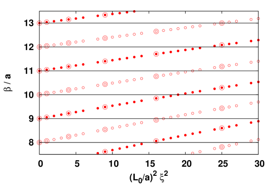
Figure 1: Inverse temperature values that become accessible with the use of shifted boundary conditions at a fixed lattice spacing $a$ and for different values of $L_{0}/a$. The inverse temperatures accessible with a shift in a single direction, $\bm{\xi}=(\xi_{1},0,0)$, are marked by a double circle.

The possibility of varying the temperature by changing either $L_{0}/a$ or $\bm{\xi}$ allows for a fine scan of the temperature axis at fixed lattice spacing. This is illustrated in Fig. 1, where it is also compared with the standard procedure of varying $L_{0}/a$ only. This fact may turn out to be useful in all those cases where the temperature needs to be changed in small steps, e.g. study of phase transitions etc.

4.2 Renormalization of the energy-momentum tensor

In the continuum, the charges associated with translational symmetries, i.e. the total energy and momentum fields, do not need any ultraviolet renormalization thanks to the Ward identities that they satisfy, for a recent discussion see Ref. [2] and references therein. On the lattice, however, translational invariance is broken down to a discrete group and the standard charge discretizations acquire finite ultraviolet renormalizations. The energy-momentum field $T_{\mu\nu}$ is a symmetric rank-two tensor. Its traceless part is an irreducible representation of the SO(4) group. On the lattice, however, the diagonal and off-diagonal components of this multiplet belong to different irreducible representations of the hypercubic lattice symmetry group and therefore renormalize in a different way. In SU($N$) Yang–Mills theory, they both renormalize multiplicatively. The WIs can be enforced on the lattice to compute the overall renormalization constant $Z_{T}$ of the multiplet, and the relative normalization $z_{{}_{T}}$ between the off-diagonal and the diagonal components [7],

$$T_{01}^{\rm R}=Z_{{}_{T}}T_{01},\qquad\qquad T_{00}^{\rm R}-T_{11}^{\rm R}=Z_{{}_{T}}\,z_{{}_{T}}\,(T_{00}-T_{11}),\qquad{\rm etc.}$$ (22)

where the fields with a superscript ‘R’ are the renormalized ones. There are many ways to implement this strategy in practice. A possible choice is to require a primitive matrix

$$V_{T}=\left(\begin{array}[]{c@{~~}c@{~~}c@{~~}c}L_{0}\hfil~{}~{}&0\hfil~{}~{}&0\hfil~{}~{}&0\\ \frac{L_{0}}{2}\hfil~{}~{}&\frac{5}{2}L_{0}\hfil~{}~{}&0\hfil~{}~{}&0\\ 0\hfil~{}~{}&0\hfil~{}~{}&L\hfil~{}~{}&0\\ 0\hfil~{}~{}&0\hfil~{}~{}&0\hfil~{}~{}&L\end{array}\right)\;$$ (23)

and compute $z_{{}_{T}}$ and $Z_{T}$ as (see also Ref. [8])

$$z_{{}_{T}}=\frac{3}{2}\frac{\langle T_{01}\rangle_{V_{T}}}{\langle T_{00}\rangle_{V_{T}}-\langle T_{11}\rangle_{V_{T}}}\;,\qquad Z_{T}=\frac{1}{L_{0}\langle T_{0k}\rangle_{V_{T}}}\frac{\partial}{\partial\xi_{k}}\ln Z(V_{T})\;.$$ (24)

Alternatively $Z_{T}$ can be determined from ($x_{0}\neq y_{0}$, $x_{2}\neq y_{2}$)

$$\frac{Z_{T}}{z_{{}_{T}}}=\frac{\langle T_{00}\rangle_{V_{T}}-\langle T_{22}\rangle_{V_{T}}}{L_{0}\,\langle{\overline{T}}_{02}(x_{0})\,T_{02}(y)\rangle_{V_{T},c}-L\,\langle{\widetilde{T}}_{02}(x_{2})\,T_{02}(y)\rangle_{V_{T},c}}\;.$$ (25)

Being fixed by WIs, the finite renormalization constants $Z_{T}$ and $z_{{}_{T}}$ depend on the bare coupling constant only. Up to discretization effects, they are independent of the kinematics used to impose them, e.g. the volume, the temperature, the shift parameter, $x_{0}$ etc. Ultimately which WIs and/or kinematics yield the most accurate results must be investigated numerically.

4.3 Calculation of the entropy and specific heat

Once the relevant renormalization constants are determined, the entropy density can be computed from the expectation value of $T_{0k}$ on a lattice with shifted boundary conditions,

$$s=-\frac{Z_{T}L_{0}(1+{\bm{\xi}}^{2})^{3/2}}{\xi_{k}}\,\langle T_{0k}\rangle_{\bm{\xi}}\;,\qquad\xi_{k}\neq 0\;,$$ (26)

by performing simulations at a single inverse temperature value $\beta=L_{0}\sqrt{1+\bm{\xi}^{2}}$, and at a volume large enough for finite-size effects to be negligible. The latter are exponentially small in $(ML)$, where $M$ is the lightest screening mass of the theory [3]. For the theory discretized with the Wilson action and for the ‘clover’ form of the lattice field strength tensor, discretization effects turn out to be remarkably small [3, 9]. Once the entropy has been computed at various values of $\beta$, the pressure can be computed by integrating $s$ in the temperature. The ambiguity left due to the integration constant is consistent with the fact that $p$ is defined up to an arbitrary additive renormalization constant.

The entropy density could also be computed directly from Eq. (20) without the need for fixing the multiplicative renormalization constant. This would require, however, the computation of the two-point correlation functions in a large volume. The latter can also be used to access the specific heat of the system by using Eq (21).

We thank M. Pepe and D. Robaina for interesting discussions. This work was partially supported by the Center for Computational Sciences in Mainz, by the DFG grant ME 3622/2-1 Static and dynamic properties of QCD at finite temperature, by the MIUR-PRIN contract 20093BMNPR, and by the INFN SUMA project.

References

- [1] L. Giusti and H. B. Meyer, Phys. Rev. Lett. 106 (2011) 131601 [arXiv:1011.2727].
- [2] L. Giusti and H. B. Meyer, JHEP 1111 (2011) 087 [arXiv:1110.3136].
- [3] L. Giusti and H. B. Meyer, JHEP 1301 (2013) 140 [arXiv:1211.6669].
- [4] H. Ott Z. Phys. 175 (1963) 70.
- [5] H. Arzelies Nuovo Cimento 35 (1965) 792.
- [6] M. Przanowski and J. Tosiek, Physica Scripta 84 (2011), no. 5 055008.
- [7] S. Caracciolo, G. Curci, P. Menotti, and A. Pelissetto, Annals Phys. 197 (1990) 119.
- [8] D. Robaina and H. B. Meyer, these proceedings [arXiv:1310.6075].
- [9] L. Giusti and M. Pepe, PoS (LATTICE 2013) 489.