Galois conjugates of entropies of real unimodal maps

1. Introduction

A classical way to measure the complexity in the orbit structure of a dynamical system $f:X\to X$ is its topological entropy $h(f)$. When the system has a Markov partition, then its topological entropy is the logarithm of an algebraic number: in fact, if we call growth rate of $f$ the quantity

$$s(f):=e^{h(f)}$$

then $s(f)$ is the leading eigenvalue of the transition matrix associated to the partition. In this paper, we are interested in the relationship between the dynamical properties of $f$ and the algebraic properties of its growth rate.

By the Perron-Frobenius theorem it follows immediately that $s(f)$ must be a weak Perron number, i.e. a real algebraic integer which is at least as large as the modulus of all its Galois conjugates. In [Th], Thurston asked the converse

Question. What algebraic integers arise as growth rates of dynamical systems with a Markov partition?

The question makes sense in several contexts, e.g. for pseudo-Anosov maps of surfaces, as well as automorphisms of the free group. In this note we shall focus on multimodal maps, i.e. continuous interval maps which have finitely many intervals of monotonicity (e.g., polynomial maps). In this context, the condition of having a Markov partition can be reformulated by saying that a multimodal map is postcritically finite if the orbits of all its critical points are finite. For these maps, the above question was settled in the following

Theorem 1.1 ([Th]).

The set of all growth rates of postcritically finite multimodal interval maps coincides with the set of all weak Perron numbers.

The question becomes more subtle when one restricts oneself to maps of a given degree. In particular, in the case of degree two, Thurston looked at the algebraic properties of growth rates of postcritically finite real quadratic polynomials; remarkably, he found out that the union of all their Galois conjugates exhibits a rich fractal structure (Figure 1). Moreover, he claimed that such a fractal set is path-connected. In this note we will formally introduce this object and study its geometry.

Let $f_{c}(z):=z^{2}+c$ be a real quadratic polynomial, with $c\in[-2,1/4]$. We shall call the map $f_{c}$ superattracting if the critical point $z=0$ is periodic. Each superattracting parameter is the center of a hyperbolic component in the Mandelbrot set; let us denote by $M_{0}$ the set of all superattracting parameters. Moreover, if $\lambda$ is an algebraic number, we shall denote by $Gal(\lambda)$ the set of Galois conjugates of $\lambda$, i.e. the set of roots of its minimal polynomial.

Definition 1.2.

We shall call entropy spectrum $\Sigma$ the closure of the set of Galois conjugates of growth rates of superattracting real quadratic polynomials:

$$\Sigma:=\overline{\bigcup_{c\in M_{0}\cap\mathbb{R}}Gal(s(f_{c}))}.$$

The set $\Sigma$ is a compact subset of $\mathbb{C}$, and it displays a lot of structure (see Figures 1, 3). We will establish the following:

Theorem 1.3.

The set $\Sigma$ is path-connected and locally connected.

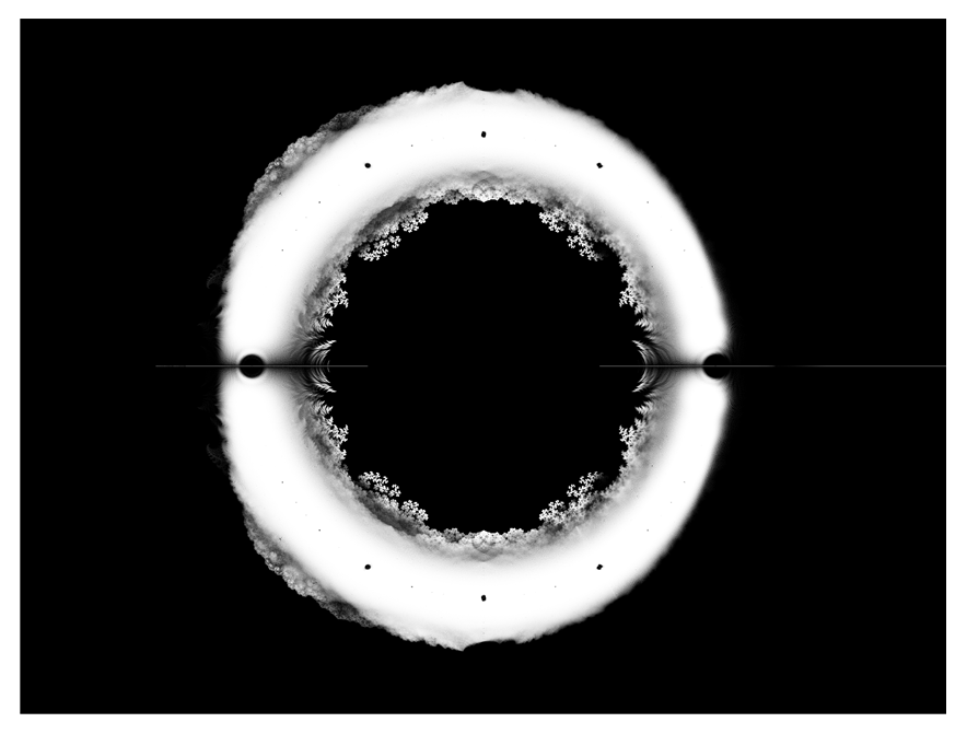
Figure 1. The entropy spectrum $\Sigma$ for real quadratic polynomials.

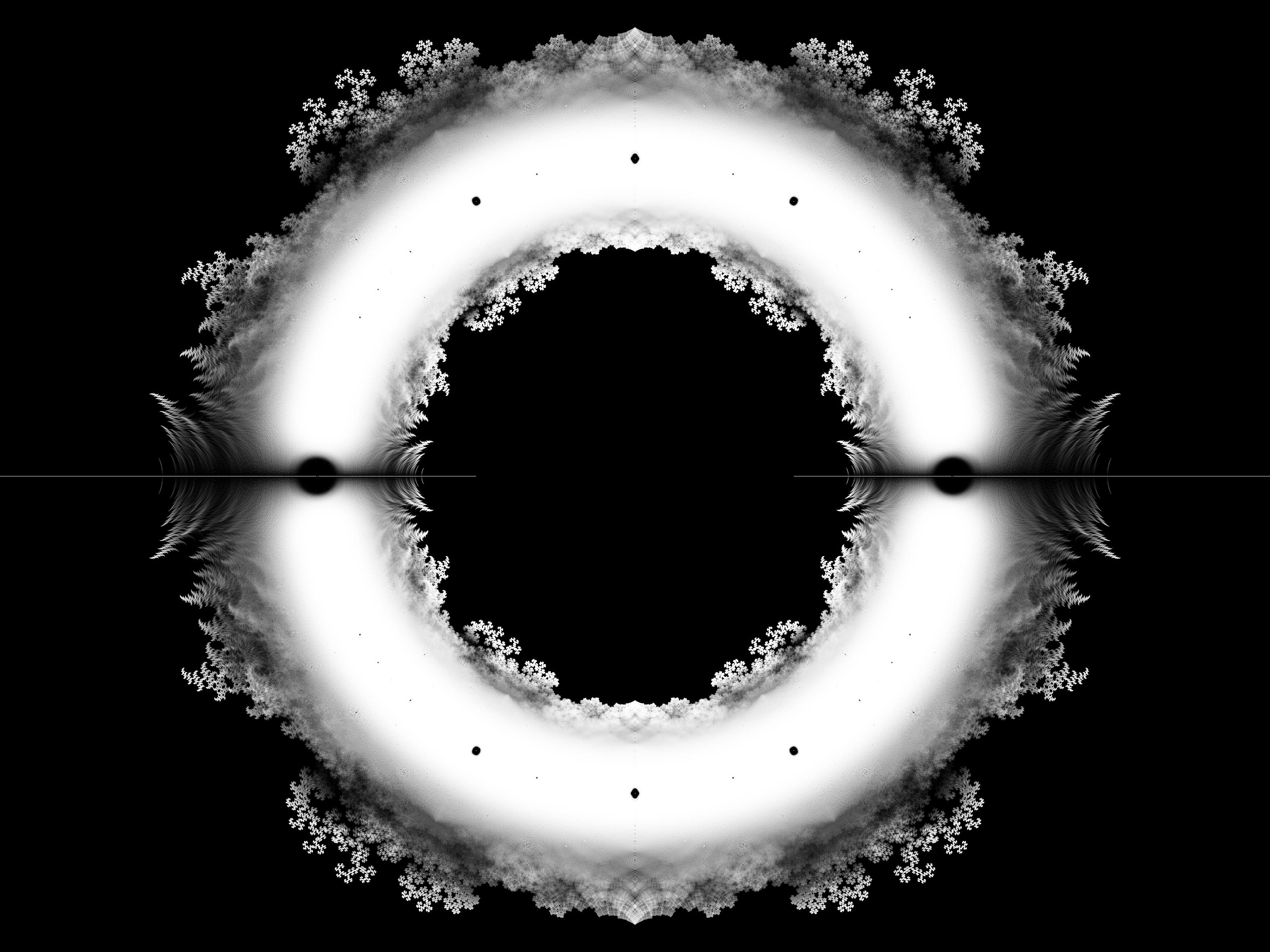
Figure 2. The set of zeros of all polynomials with coefficients $\pm 1$.

The proof follows the techniques used by Bousch [B1], [B2] and Odlyzko-Poonen [OP] to prove the path-connectivity of the sets of zeros of certain power series with prescribed coefficients (see Figure 2). The reason of this connection is the kneading theory of Milnor and Thurston [MT]. Indeed, they showed that for each map $f_{c}$ one can construct a certain power series $K_{c}(t)$, known as kneading determinant, in such a way that the inverse of the growth rate of $f_{c}$ is a zero of $K_{c}(t)$. Thus, the set $\Sigma$ is closely related to the set $\Sigma_{kn}$ of all zeros of all kneading determinants (see section 3).

The proof of the main theorem will be split in several parts. We shall denote by $\mathbb{D}:=\{z\in\mathbb{C}\ :\ |z|<1\}$ the unit disk in the complex plane, and by $\mathbb{E}:=\{z\in\mathbb{C}\ :\ |z|>1\}$ the part of the plane outside the closed unit disk. The part of $\Sigma$ inside the unit disk will be analyzed by comparing it to the set $\Sigma_{\pm 1}$ of zeros of all polynomials with coefficients $\pm 1$ (section 5); in fact, we shall prove that $\Sigma$ and $\Sigma_{\pm 1}$ coincide inside the unit disk (Proposition 5.2). On the other hand, the part outside the disk will require a different analysis. Namely, we shall first analyze the kneading set $\Sigma_{kn}$, proving that the intersection $\Sigma_{kn}\cap\mathbb{E}$ is connected and locally connected (section 3). Finally, in order to prove the same statement about $\Sigma$, we shall then address the question of which polynomials given by the kneading theory are in fact irreducible. As we shall see (section 7.2), this question is closely related to the combinatorics of renormalization. We shall also prove that $\Sigma$ and $\Sigma_{kn}$ both contain a neighbourhood of the unit circle (section 6), completing the proof.

Finally, it is worth pointing out that fractal sets similar to $\Sigma$ can be constructed using other families of quadratic polynomials. In particular, one can consider for each postcritically finite quadratic polynomial $f$ the restriction of $f$ to its Hubbard tree, and its growth rate will be an algebraic number. Thus, one can construct for instance the set of Galois conjugates of growth rates of superattracting maps along any vein in the Mandelbrot set (see the Appendix for some pictures), or even consider all centers of all hyperbolic components at once. The corresponding questions about the geometry of these sets are still open.

Acknowledgements

All the essential ideas go back to W. Thurston: this paper wants to be a step towards a more complete understanding of his last works, which are extremely rich and deserve to be completed in detail. I wish to thank C. T. McMullen for putting me in contact with Thurston’s work, in particular the preprint [Th]. I also thank S. Koch, Tan Lei and B. Poonen for useful conversations.

2. Review of kneading theory

Let $f(z)=z^{2}+c$. We define the sign $\epsilon(x)$ of a point $x\neq 0$ with respect to the partition given by the critical point to be

$$\epsilon(x):=\left\{\begin{array}[]{ll}-1&\textup{ if }x<0\\ +1&\textup{ if }x>0.\end{array}\right.$$

Moreover, for each $k\geq 1$ we define $\eta_{k}(x):=\epsilon(x)\epsilon(f(x))\dots\epsilon(f^{k-1}(x))$. If the forward orbit of $x$ does not contain the critical point, then the kneading series of $x$ is defined as

$$K(x,t):=1+\sum_{k=1}^{\infty}\eta_{k}(x)t^{k}.$$

We now associate to each map $f_{c}$ a power series $K_{c}(t)$, known as kneading determinant. If the critical point is not periodic, then we define

$$K_{c}(t):=K(c,t).$$

Otherwise, we define

$$K_{c}(t):=\lim_{x\to c^{+}}K(x,t)$$

where the limit is taken over all subsequences such that $x$ does not map to the critical point. The series $K_{c}(t)$ converges in the disk of unit radius, and its smallest real positive root is the inverse of the growth rate:

Theorem 2.1 ([MT]).

Let $s$ be the growth rate of $f_{c}$. Then the function $K_{c}(t)$ has no zeros on the interval $[0,1/s)$, and if $s>1$ we have

$$K_{c}(1/s)=0.$$

If the critical point is periodic of period $p$, then the coefficients of $K_{c}(t)$ are periodic, so the function $K_{c}(t)$ can be written in the form

$$K_{c}(t)=\frac{P(t)}{1-t^{p}}$$

where $P(t)$ is a polynomial of degree $p-1$ with coefficients in $\{\pm 1\}$. We shall call $P(t)$ the kneading polynomial of $f_{c}$. A power series is admissible if it is the kneading determinant of some real quadratic polynomial. Similarly, a polynomial $P(t)$ of degree $n$ is admissible if the power series expansion of $P(t)/(1-t^{n+1})$ is admissible. Admissible power series can be characterized in terms of the action of the shift operator on its coefficients. In order to recall the criterion, let us say that a formal power series $\phi(t)$ is positive if its first non-zero coefficient is positive, and that two formal power series satisfy $\phi_{1}(t)<\phi_{2}(t)$ if $\phi_{2}(t)-\phi_{1}(t)$ is positive. Moreover, the absolute value $|\phi(t)|$ of a formal power series will equal $\phi(t)$ is $\phi(t)\geq 0$ and $-\phi(t)$ if $\phi(t)<0$. The admissibility criterion is the following.

Theorem 2.2 ([MT], Theorem 12.1).

Let

$$\phi(t):=1+\sum_{k=1}^{\infty}\epsilon_{k}t^{k}$$

be a power series, with $\epsilon_{k}\in\{\pm 1\}$. The power series $\phi(t)$ is admissible if and only if

$$\phi(t)\leq|\sum_{k=n}^{\infty}\epsilon_{k}t^{k}|$$

for each $n\geq 1$.

In particular, the theorem immediately implies the following sufficient condition, which we will use later.

Corollary 2.3.

Let

$$\phi(t):=1+\sum_{k=1}^{\infty}\epsilon_{k}t^{k}$$

be a power series, with $\epsilon_{k}\in\{\pm 1\}$ and $\epsilon_{1}=-1$. Define the initial runlength $N$ to be the number of consecutive equal symbols at the beginning of the sequence of coefficients:

$$N:=\max\{k\geq 1:\epsilon_{1}=\epsilon_{2}=\dots=\epsilon_{k}\}$$

and the maximal runlength $M$ to be the cardinality of the largest sequence of consecutive equal symbols, excluding the first one:

$$M:=\max\{k\geq 1:\epsilon_{n}=\epsilon_{n+1}=\dots=\epsilon_{n+k-1}\textup{ for some }n\geq N+1\}.$$

If $N>M$, then the power series $\phi(t)$ is admissible.

Moreover, let us recall that kneading determinants behave nicely under tuning operations. Indeed, let $f_{c_{0}}$ be a superattracting real polynomial of period $p$ and kneading determinant $K_{c_{0}}(t)=P_{c_{0}}(t)/(1-t^{p})$, and $f_{c_{1}}$ another real polynomial. Then their Douady-Hubbard tuning $f_{c_{2}}=f_{c_{0}}\star f_{c_{1}}$ has kneading polynomial (see [Do1])

(1) $$P_{c_{2}}(t)=P_{c_{1}}(t^{p})P_{c_{0}}(t).$$

Let us conclude the section with a few basic observations on the geometry of $\Sigma$.

Lemma 2.4.

We have the inclusion

$$\Sigma\subseteq\{z\ :\ 1/2\leq|z|\leq 2\}.$$

Proof.

Let $P(t)=\sum_{k=0}^{n}\epsilon_{k}t^{k}$, with $|\epsilon_{k}|=1$. Then if $|t|<1/2$ we have

$$|P(t)|\geq 1-\sum_{k=1}^{n}2^{-n}>0$$

so there is no zero inside the disk of radius $1/2$. Taking the reciprocal polynomial proves that there is no root of modulus larger than $2$. The claim then follows because all kneading polynomials for superattracting maps have coefficients of unit modulus. ∎

Finally, one of the main results of Milnor and Thurston’s kneading theory is the following monotonicity of entropy.

Theorem 2.5 ([MT]).

The growth rate $s(f_{c})$ of $f_{c}(z):=z^{2}+c$ is a continuous, decreasing function of the parameter $c\in[-2,1/4]$.

Since $s(f_{1/4})=1$ and $s(f_{-2})=2$, by the density of hyperbolic components on the real line we get immediately the

Corollary 2.6.

The set $\Sigma$ contains the real interval $[1,2]$.

3. Outside the unit disk : the kneading spectrum

For the sake of exposition, let us first analyze a set which is related to $\Sigma$. Let us define the kneading spectrum $\Sigma_{kn}$ for real unimodal maps as the set of (inverses of) all zeros of kneading determinants: more precisely, we set

$$\Sigma_{kn}:=\overline{\{s\in\mathbb{C}^{*}\ :\ K_{c}(1/s)=0\textup{ for some superattracting }f_{c}\}}.$$

Since the growth rates are zeros of the reciprocals of kneading polynomials, then we have the inclusion

$$\Sigma\subseteq\Sigma_{kn}.$$

However, it is not always true that kneading polynomials are irreducible (indeed, they are not inside small copies of the Mandelbrot set, see section 7.2), so it is not obvious that the two sets are the same.

In this section, we shall prove the following result.

Proposition 3.1.

The set $\Sigma_{kn}\cap\{z:|z|\geq 1\}$ is connected, and the set $\Sigma_{kn}\cap\{z:|z|>1\}$ is locally connected.

Let us first observe that the set $\Sigma_{kn}$ has the remarkable property of being closed under taking $n^{th}$-roots, and this is precisely because of renormalization.

Lemma 3.2.

If $s\in\mathbb{C}^{*}$ belongs to $\Sigma_{kn}$ and $t^{n}=s$ for some $t\in\mathbb{C}^{*}$ and $n$ a positive integer, then $t$ also belongs to $\Sigma_{kn}$. As a consequence, $\Sigma_{kn}$ contains the unit circle $S^{1}$.

Proof.

Let $s$ be such that $K_{c}(1/s)=0$ with $f_{c}(z)$ a superattracting real quadratic polynomial, and let $t\in\mathbb{C}$ such that $t^{n}=s$. Now let us pick $f_{c_{1}}$ a superattracting real quadratic polynomial with critical orbit of period $n$, and construct the tuned map $f_{c_{2}}:=f_{c_{1}}\star f_{c}$. Then by equation (1) we have that $K_{c_{2}}(z)=K_{c}(z^{n})P_{c_{1}}(z)$, and by evaluating it for $z=t^{-1}$ we get $K_{c_{2}}(t^{-1})=K_{c}(t^{-n})P_{c_{1}}(t^{-1})=0$ since $t^{-n}=s^{-1}$, hence $t$ also belongs to $\Sigma_{kn}$. The claim then follows by taking closures. ∎

Let us first observe that, since periodic kneading sequences are dense in the set of admissible kneading sequences, we can drop the closure if we admit kneading determinants of all real maps: that is, we have the identity

$$\Sigma_{kn}\cap\mathbb{E}=\{s\in\mathbb{E}\ :\ K_{c}(1/s)=0\textup{ for some }c\in[-2,1/4]\}.$$

The fundamental idea then is that we can associate to each parameter $c$ a discrete subset of the disk, namely the set of zeros of $K_{c}(t)$, in a continuous way, and we are interested in studying the union of all such sets. It is thus natural to consider the three-dimensional set

(2) $$\widehat{\Sigma}:=\{(c,z)\in[-2,1/4]\times\mathbb{D}\ s.t.\ K_{c}(z)=0\}$$

which “fibers” over $[-2,1/4]$ by taking the projection $\pi_{1}$ onto the first coordinate, and each fiber of $\pi_{1}$ is the set of zeros of $K_{c}(t)$.

We will actually prove that $\widehat{\Sigma}$ is connected and locally connected: the Proposition then follows since the set $\Sigma_{kn}\cap\mathbb{E}$ is just obtained by taking the projection of $\widehat{\Sigma}$ onto the second coordinate, and then inverting through the unit circle via the map $z\mapsto 1/z$.

Let $Com\ V$ denote the space of compact subsets of a compact metric space $V$, with the Hausdorff topology. Moreover, let $\widetilde{\mathbb{D}}:=\mathbb{D}\cup\{\infty\}$ be the one-point compactification of the unit disk. If $f$ is a holomorphic function in the unit disk, the trace of $f$ is defined as the set of zeros of $f$:

$$\textup{tr }f:=\{z\in\mathbb{D}\ :\ f(z)=0\}\cup\{\infty\}.$$

By Rouché’s theorem, the map $\textup{tr }f:\mathcal{O}(\mathbb{D})\to Com\ \widetilde{\mathbb{D}}$ is continuous at $f$ as long as $f$ is not identicallly $0$. Let us now verify continuity for kneading determinants:

Proposition 3.3.

The map $\textup{Tr}:[-2,1/4]\to Com\ \widetilde{\mathbb{D}}$ given by

$$\textup{Tr}(c):=\{z\in\mathbb{D}\ :\ K_{c}(z)=0\}\cup\{\infty\}$$

is continuous in the Hausdorff topology.

Proof.

Let us consider the map $\Phi:[-2,1/4]\to\mathcal{O}(\mathbb{D})$ given by $\Phi(c):=K_{c}(t)$. If the critical point is not periodic for $f_{c}$, then $\Phi$ is continuous at $c$ because it is continuous in the topology of formal power series. Otherwise, if the critical point has period $p$, we have

$$\lim_{s\to c^{+}}\Phi(s)=\frac{P(t)}{1-t^{p}}\qquad\lim_{s\to c^{-}}\Phi(s)=\frac{P(t)}{1+t^{p}}$$

where $P(t)$ is a polynomial of degree $p-1$; thus the two limit functions have the same zero sets inside the unit disk, so the map is still continuous. ∎

Lemma 3.4 ([B2]).

Let $\Lambda$ a topological space and $V$ a compact metric space. Let $t:\Lambda\to Com\ V$ be a continuous map, and denote as $t(\Lambda)$ the union

$$t(\Lambda):=\bigcup_{\lambda\in\Lambda}t(\lambda).$$

Then the following are true:

1. suppose $\Lambda$ is connected and there exists $\lambda_{0}\in\Lambda$ such that $t(\lambda_{0})$ is connected; then $t(\Lambda)$ is connected.

2. Suppose $\Lambda$ is compact and locally connected, and let $U\subset V$ be an open subset such that $t(\lambda)\cap U$ is discrete for each $\lambda\in\Lambda$. Then $t(\Lambda)\cap U$ is locally connected.

Proof of Proposition 3.1.

We apply the Lemma to $\Lambda=[-2,1/4]$ (which is obviously connected and locally connected), $V=\widetilde{\mathbb{D}}$, $U=\mathbb{D}$. Since $K_{0}(t)$ has no zeros inside the unit disk, then $\textup{Tr}(0)=\{\infty\}$ is connected, so by (1) the one-point compactification of $\Sigma_{kn}\cap\mathbb{E}$ is connected. Since by Lemma 3.2 $\Sigma_{kn}$ contains $S^{1}$ which is connected, then $(\Sigma_{kn}\cap\mathbb{E})\cup S^{1}$ is also connected. Since no kneading determinant is identically zero, for each $c$ the set of zeros of $K_{c}(t)$ inside the unit disk is discrete, so by (2) we get that that $\Sigma_{kn}\cap\mathbb{E}$ is locally connected. ∎

A (direct) proof of the path-connectivity of $\Sigma_{kn}$ will be given in section 7.1. It is worth mentioning that a three-dimensional object very close to $\widehat{\Sigma}$ appears in Thurston’s paper [Th], where it is called the “master teapot”.

4. Irreducible polynomials

In order to study the Galois conjugates of growth rates we need to find their minimal polynomials. In particular, since we know that kneading polynomials vanish on the growth rate, they coincide with the minimal polynomials once we prove they are irreducible. To construct irreducible polynomials we shall use the next two algebraic lemmas. The following observation is due to B. Poonen.

Lemma 4.1.

Let $d=2^{n}-1$ with $n\geq 1$, and choose a sequence $\epsilon_{0},\epsilon_{1},\dots,\epsilon_{n}$ with each $\epsilon_{k}\in\{\pm 1\}$, such that $\sum_{k=0}^{d}\epsilon_{k}\equiv 2\ \mod 4$. Then the polynomial

$$f(x):=\epsilon_{0}+\epsilon_{1}x+\dots+\epsilon_{d}x^{d}$$

is irreducible in $\mathbb{Z}[x]$.

Proof.

We apply Eisenstein’s criterion to $g(x):=f(x+1)$. Indeed, reducing modulo $2$,

$$xf(x+1)\equiv\sum_{k=0}^{d}x(x+1)^{k}\equiv(x+1)^{d+1}-1\equiv x^{d+1}$$

where in the last equation we used that $d+1$ is a power of $2$. Thus, we have $g(x)\equiv x^{d}$ modulo $2$, while $g(0)=\sum_{k=0}^{d}\epsilon_{k}$ is divisible by $2$ but not by $4$ by hypothesis and Eisenstein’s criterion can be applied. ∎

Lemma 4.2.

Let $f(x):=1+\sum_{k=1}^{d}\epsilon_{k}x^{k}$ be a polynomial, with $\epsilon_{k}\in\{\pm 1\}$ for all $1\leq k\leq d$ and $\epsilon_{k}=-1$ for some $k$. If $f(x)$ is irreducible in $\mathbb{Z}[x]$, then for all $n\geq 1$ the polynomial $f(x^{2^{n}})$ is irreducible in $\mathbb{Z}[x]$.

Proof.

Suppose by contradiction $n\geq 1$ is the minimal integer for which $f(x^{2^{n}})$ is not irreducible. Thus, there exists a (unique) factorization

$$f(x^{2^{n}})=g_{1}(x)\dots g_{r}(x)$$

where $g_{1}(x),\dots,g_{r}(x)$ are irreducible polynomials with $g_{i}(0)=1$ for each $i$. By substituting $x$ with $-x$, we get

$$f(x^{2^{n}})=g_{1}(-x)\dots g_{r}(-x)$$

so by uniqueness of the factorization there exists an involution $\sigma:\{1,\dots,r\}\to\{1,\dots,r\}$ such that for each $i$ we have $g_{i}(-x)=g_{\sigma(i)}(x)$. If the involution $\sigma$ has a fixed point $i$, then $g_{i}(x)$ is of the form $g_{i}(x)=h_{1}(x^{2})$ for some $h_{1}(x)\in\mathbb{Z}[x]$, which implies that $f(x^{2^{n}})$ can be factored as

$$f(x^{2^{n}})=h_{1}(x^{2})h_{2}(x^{2})\qquad h_{1}(x),h_{2}(x)\in\mathbb{Z}[x]$$

so $f(x^{2^{n-1}})$ is also reducible, contradicting the minimality of $n$. Hence the involution $\sigma$ has no fixed point and, by grouping together the factors $g_{k}(x)$, we have the factorization

(3) $$f(x^{2^{n}})=g(x)g(-x)$$

for some $g(x)\in\mathbb{Z}[x]$. We shall now see that this is impossible, by comparing coefficients on both sides of equation (3). Let us denote the coefficients by $f(x^{2^{n}}):=\sum_{k=0}^{2^{n}d}b_{k}x^{k}$ and $g(x):=\sum_{k=0}^{2^{n-1}d}a_{k}x^{k}$. Let us look at equation (3). Since $a_{0}^{2}=b_{0}=1$, then $a_{0}=\pm 1$. For each $1\leq k\leq 2^{n-1}d$, the coefficient of $x^{2k}$ is of type

(4) $$b_{2k}=\sum_{j=j_{0}}^{k-1}\pm 2a_{j}a_{2k-j}\pm a_{k}^{2}$$

where $j_{0}:=\max\{0,2k-2^{n-1}d\}$. As a consequence, we see that $a_{k}$ is even if and only if $b_{2k}$ is even. Thus we get the following congruences:

(5) $$\left\{\begin{array}[]{ll}a_{j}\equiv 0\mod 2&\textup{ for }1\leq j\leq 2^{n-2}\textup{ (if }n\geq 2\textup{)}\\ a_{j2^{n-1}}\equiv 1\mod 2&\textup{ for }1\leq j\leq d.\end{array}\right.$$

We now have two cases:

• Suppose $n\geq 2$. Then if we look at equation (4) for $k=2^{n-2}$, we get the equality

  $$2a_{0}a_{2^{n-1}}+\sum_{j=1}^{2^{n-2}-1}\pm 2a_{j}a_{2^{n-1}-j}\pm a_{2^{n-2}}^{2}=0.$$

  By equation (5), every term in the sum except possibly for the first one is multiple of $4$, so the first term $2a_{0}a_{2^{n-1}}=\pm 2a_{2^{n-1}}$ must also be multiple of $4$, so $a_{2^{n-1}}$ is even. However, this contradicts the second line of equation (5).

• Suppose $n=1$. Then from equation (5) we have for each $1\leq k\leq d$ that $a_{k}$ is odd, and equation (4) becomes of the form

  $$b_{2k}=2N_{k}+(-1)^{k}a_{k}^{2}$$

  where $N_{k}$ has the same parity as the number of terms under the summation symbol in (4), which is $\min\{k,d-k\}$. Now, by analyzing the previous equation modulo $4$ we realize that $b_{2k}$ cannot be $-1$ for any $1\leq k\leq d/2$, so we must have $b_{2k}=1$ for all $1\leq k\leq d/2$. Moreover, for $k>d/2$ either $d$ is even and $b_{2k}=1$ for all $d/2\leq k\leq d$, or $d$ is odd and $b_{2k}=-1$ for all $d/2\leq k\leq d$. In the first case we contradict the initial hypothesis on $f(x)$ since all its coefficients equal $+1$; in the second case, we also get a contradiction because we obtain that $f(x)=(\sum_{k=0}^{\frac{d-1}{2}}x^{k})(1-x^{\frac{d+1}{2}})$ is not irreducible.

∎

Note that the condition on the coefficients of $f(x)$ not being all equal is essential: indeed, the polynomial $f(x):=\sum_{k=0}^{p-1}x^{k}$ can be irreducible (e.g. for $p=5$), but $f(x^{2})$ never is. Related issues on irreducibility and its relationship to renormalization will be discussed in sections 7.2 and 7.3.

5. Inside the disk: roots of polynomials with coefficients $\pm 1$

Since the series $K_{c}(t)$ need not converge outside the unit disk, then the set of zeros of $K_{c}(t)$ outside the disk need not (and probably does not) vary continuously as a function of $c$. However, it turns out that the set $\Sigma\cap\mathbb{D}$ coincides with another set which has a natural parameterization by a path-connected set. Let $\Sigma_{\pm 1}$ be the set of zeros of power series with coefficients $+1$ or $-1$:

$$\Sigma_{\pm 1}:=\left\{s\in\mathbb{D}\ :\ \sum_{k=1}^{\infty}\epsilon_{k}s^{k}=0\textup{ for some }\epsilon_{k}\in\{-1,+1\}^{\mathbb{N}}\right\}.$$

The set $\Sigma_{\pm 1}$ was considered by Bousch [B1], [B2] in connection with the dynamics of certain iterated function systems (IFS). In fact, for each $s\in\mathbb{D}$, the IFS given by $z\mapsto sz\pm 1$ has a compact attractor $K_{s}$, and a parameter $s\in\mathbb{D}$ belongs to $\Sigma_{\pm 1}$ if and only if $K_{s}$ contains the “critical point” $z=0$.

The set $\Sigma_{\pm 1}$ is naturally parameterized by the Cantor set $\{\pm 1\}^{\mathbb{N}}$; by producing a path-connected quotient of the Cantor set which parameterizes $\Sigma_{\pm 1}$, Bousch proved the following

Theorem 5.1.

The set $\Sigma_{\pm 1}$ is path-connected and locally connected.

We shall now see that the intersections of the two sets with the unit disk are the same:

Proposition 5.2.

We have the equality

$$\Sigma\cap\mathbb{D}=\Sigma_{\pm 1}\cap\mathbb{D}.$$

Then, using Theorem 5.1, we get the

Corollary 5.3.

The set $\Sigma\cap\mathbb{D}$ is path-connected and locally connected.

Proof of Proposition 5.2.

Since the kneading determinants have coefficients $\pm 1$, it is clear that $\Sigma\cap\mathbb{D}\subseteq\Sigma_{\pm 1}\cap\mathbb{D}$. In order to prove the other inclusion, let

$$\phi(t):=\sum_{k=0}^{\infty}\epsilon_{k}t^{k}$$

be any power series with $\epsilon_{i}\in\{\pm 1\}$, and fix $n\geq 1$. Let $N_{0}$ be the maximum number of consecutive equal digits in the sequence $(\epsilon_{0},\dots,\epsilon_{n})$:

$$N_{0}:=\max\{k\ :\ \epsilon_{i}=\epsilon_{i+1}=\dots=\epsilon_{i+k-1}\textup{ for some }0\leq i\leq n-k+1\}.$$

Then for each $N>N_{0}+1$ and each choice of $\eta\in\{\pm 1\}$, the polynomial

$$P_{n}(t):=1-\sum_{k=1}^{N}t^{k}+\eta t^{N+1}+\sum_{k=0}^{n}\epsilon_{n-k}t^{N+2+k}$$

is admissible. Moreover, by construction the first $n$ coefficients of its reciprocal polynomial $Q_{n}(t):=t^{N+n+2}P_{n}(t^{-1})$ coincide with the first $n$ coefficients of $\phi(t)$; thus by Rouché’s theorem each zero of $\phi(t)$ inside the unit disk is approximated by a sequence of zeros of $Q_{n}(t)$. In addition, for each $n$ we can pick $N>N_{0}+1$ and such that $n+N+3$ is a power of $2$, and we are free to choose $\eta\in\{\pm 1\}$ such that $1-N-\eta+\sum_{k=0}^{n}\epsilon_{k}\equiv 2\mod 4$. This way, by Lemma 4.1 the polynomials $Q_{n}(t)$ are irreducible, so the zeros of $Q_{n}(t)$ belong to $\Sigma$ and the claim is proven. ∎

The essential idea in the previous proof is that every sequence arises as suffix of an admissible kneading sequence: note that we cannot prove such an identity for the part of $\Sigma$ outside the disk because not every sequence arises as prefix of an admissible sequence, and indeed the pictures suggest that $\Sigma$ is smaller than $\Sigma_{\pm 1}$.

6. A neighbourhood of the circle

Let us now prove that the set $\Sigma$ (hence also $\Sigma_{kn}$) contains a neighbourhood of the unit circle, as can be seen from Figure 3.

Proposition 6.1.

There exists $R>1$ such that the inclusion

$$\{z:R^{-1}<|z|<R\}\subseteq\Sigma$$

holds.

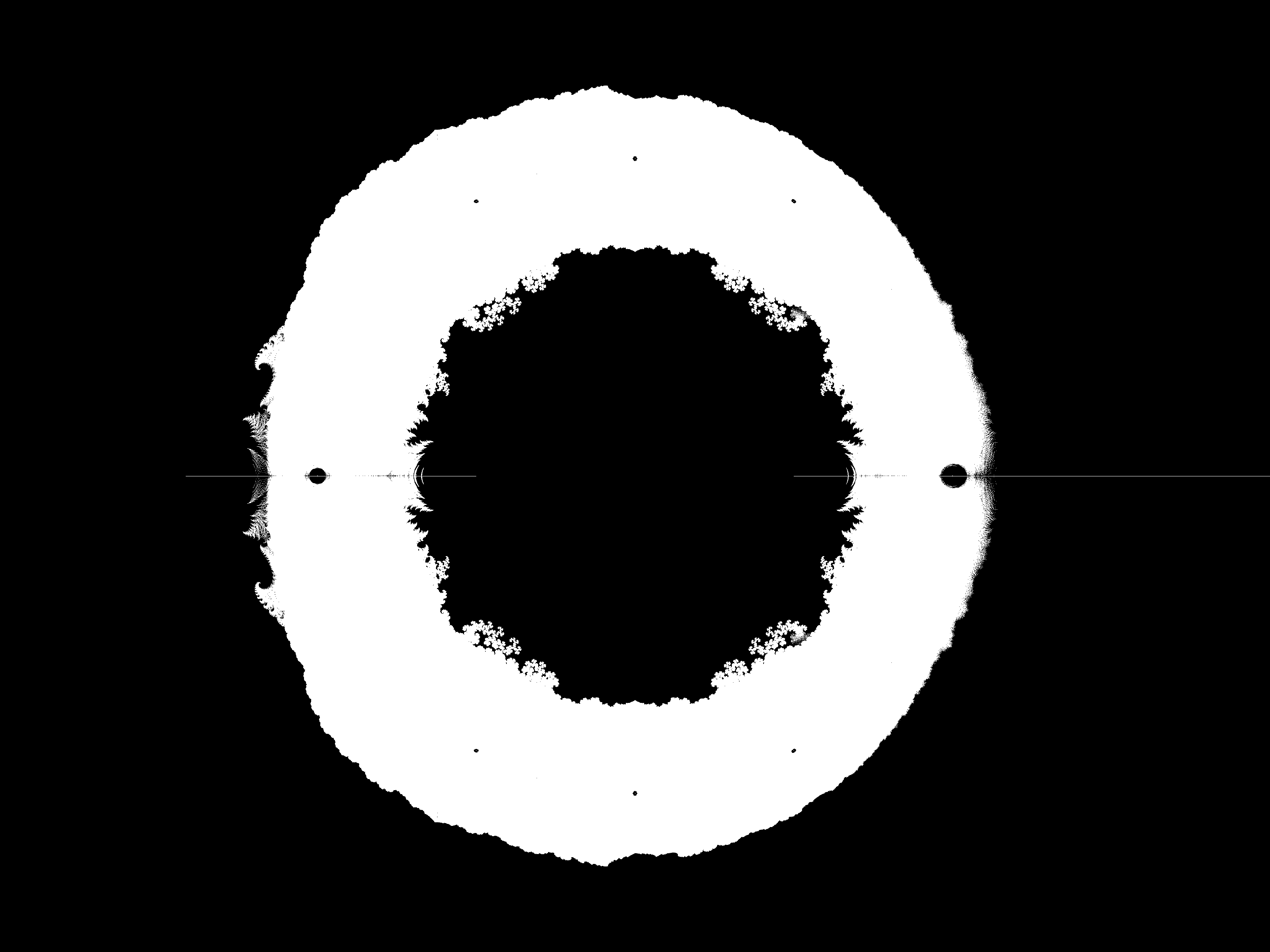
Figure 3. The boundary of the set $\Sigma$.

Bousch ([B1], Proposition 2) proves that the set $\Sigma_{\pm 1}$ contains the annulus $\{z:2^{-1/4}<|z|<1\}$, so by Proposition 5.2 it is enough to prove that $\Sigma$ contains an annulus outside the unit circle, i.e. a set of the form $\{z:1<|z|<R\}$ for some $R>1$. We shall use the following lemma (in the spirit of [OP], Lemma 3.1):

Lemma 6.2.

Let $z\in\mathbb{D}$, and $m\geq 3$ an integer. Denote by $\Lambda$ the finite set

$$\Lambda:=\{\epsilon_{0}+\epsilon_{1}z+\dots+\epsilon_{m-1}z^{m-1}\ :\ \epsilon_{k}\in\{\pm 1\}\textup{, not all }\epsilon_{k}\textup{ equal}\}$$

and suppose there exists a bounded subset $B$ of $\mathbb{C}$ and an integer $n\geq 1$ such that the following hold:

1. we have the inclusion

   $$B\subseteq\bigcup_{(w_{1},\dots,w_{n})\in\Lambda^{n}}w_{1}+w_{2}z^{m}+\dots+w_{n}z^{m(n-1)}+z^{mn}B;$$

2. $B$ contains the point $u_{2m}(z):=\frac{1-z-z^{2}-\dots-z^{2m-1}}{z^{2m}}.$

Then $z^{-1}$ belongs to $\Sigma$.

Proof.

From (2) and (1), we can write

$$u=w_{1}+w_{2}z^{m}+\dots+w_{n}z^{m(n-1)}+z^{mn}b_{1}$$

with $u=u_{2m}(z)$ and some $(w_{1},\dots,w_{n})\in\Lambda^{n}$ and $b_{1}\in B$; now, applying (1) recursively to $b_{1}$ we can find a sequence $\{b_{N}\}_{N\geq 1}$ of elements of $B$ and a sequence $\{w_{k}\}_{k\geq 1}$ of elements of $\Lambda$ such that for each $N$ we can write

$$u=\sum_{k=1}^{nN}w_{k}z^{m(k-1)}+z^{mnN}b_{N};$$

now, since $|z|<1$ and $B$ is bounded we have in the limit

$$u=\sum_{k=1}^{\infty}w_{k}z^{mk}$$

which can be rewritten as

$$0=1-z-z^{2}-\dots-z^{2m-1}+\sum_{k=2m}^{\infty}\eta_{k}z^{k}\qquad\textup{with }\eta_{k}\in\{\pm 1\}.$$

Since we initially chose the $\epsilon_{k}$ not to be all equal, then the sequence $(\eta_{k})_{k\geq 2m}$ does not contain any subsequence of $2m-1$ consecutive equal symbols, so the above power series is admissible and $z^{-1}$ belongs to the kneading spectrum $\Sigma_{kn}$.

In order to prove that $z^{-1}$ belongs to $\Sigma$, we still need to check that we can construct a sequence of admissible, irreducible polynomials whose coefficients converge to the sequence $(\eta_{k})_{k\geq 0}$. For each $N$, let us consider the truncation $(\eta_{k})_{0\leq k\leq 2^{N}-1}$ of the sequence $\eta$: if the sum $S:=\sum_{k=0}^{2^{N}-1}\eta_{k}$ is congruent to $2$ modulo $4$, then by Lemma 4.1 the polynomial $P_{N}(t):=\sum_{k=0}^{2^{N}-1}\eta_{k}t^{k}$ is irreducible and admissible. If the sum $S$ of the coefficients is instead divisible by $4$, we can flip one of the symbols $\eta_{k}$ so that the sum becomes congruent to $2$ and the sequence remains admissible. Precisely, we can find an index $k_{0}$ with $\max\{2m,2^{N-1}\}\leq k_{0}\leq 2^{N}-1$ such that the sequence $(\eta^{\prime}_{k})_{k\geq 2m}$ defined as

$$\eta^{\prime}_{k}=\left\{\begin{array}[]{ll}\eta_{k}&\textup{if }k\neq k_{0}\\ -\eta_{k}&\textup{if }k=k_{0}\end{array}\right.$$

still has at most $2m-2$ consecutive equal symbols, so that now $\sum\eta^{\prime}_{k}\equiv 2\mod 4$ and the polynomial $P_{N}(t):=\sum_{k=0}^{2^{N}-1}\eta^{\prime}_{k}t^{k}$ is irreducible and admissible. ∎

We shall apply the lemma by taking the set $B$ to be a large ball around the origin: we shall need the following elementary lemma about convex sets, whose proof we postpone to the appendix.

Lemma 6.3.

Let $v_{1},\dots,v_{n}\in\mathbb{R}^{d}$ be non-zero vectors which span $\mathbb{R}^{d}$, and suppose that their convex hull $\Lambda$ contains the origin in its interior. Then there exists $R>0$ such that any ball $B$ of radius at least $R$ centered at the origin satisfies the inclusion

$$\overline{B}\subseteq\textup{ int }\bigcup_{i=1}^{n}(v_{i}+B)$$

where $\overline{B}$ denotes the closure and int the interior part.

Proposition 6.4.

Let $z\in S^{1}$, $z\neq\pm 1$. Then a neighbourhood of $z$ is contained in $\Sigma$.

Proof.

Given $\xi\in S^{1}$, $\xi\neq\pm 1$, let us choose an integer $m\geq 3$ and coefficients $\epsilon_{0},\epsilon_{2},\dots,\epsilon_{m-1}\in\{\pm 1\}$ such that $\xi^{m}\neq\pm 1$, the vector $v:=\sum_{k=0}^{m-1}\epsilon_{k}\xi^{k}$ is non-zero and the $\epsilon_{k}$ are not all equal. Now, the four points in the set

$$\Lambda:=\{\pm v\pm\xi^{m}v\}$$

are the vertices of a parallelogram which contains the origin in its interior, hence by Lemma 6.3 there exists a ball $B$ centered at the origin such that the inclusion

(6) $$B\subseteq\textup{ int }\bigcup_{w\in\Lambda}\left(w+\xi^{2m}B\right)$$

holds. Moreover, we can choose the radius of $B$ to be large enough so that the point $u:=\frac{1-\xi-\xi^{2}-\dots-\xi^{2m-1}}{\xi^{2m}}$ belongs to the interior of $B$. Now, we see that the conditions of Lemma 6.2 are verified for each $z\in\mathbb{D}$ in a neighbourhood of $\xi$, so by the Lemma the set $\Sigma$ contains a neighbourhood of $\xi^{-1}$ and since this holds for all $\xi\in S^{1}\setminus\{\pm 1\}$ the claim is proven. ∎

Proposition 6.5.

The points $z=\pm 1$ belong to the interior of the set $\Sigma$.

The proof in this case is a bit more complicated, so it will be postponed to the appendix. It is still based on Lemma 6.2, but we can no longer choose a large ball to play the role of the bounded set $B$: instead, as in the proof of ([OP], Proposition 3.3), we have to choose a parallelogram whose shape varies with $z$.

7. $\Sigma$ is path-connected

Let us finally turn to the proof of the following

Theorem 7.1.

The set $\Sigma\cap\{z\ :\ |z|\geq 1\}$ is path-connected.

7.1. Lifting lemma and path-connectivity

The essential idea to prove path-connectivity is that the three-dimensional set $\widehat{\Sigma}$ defined in equation (2) “fibers” over an interval which is path-connected, so we can lift continuous paths in the base to continuous paths in $\widehat{\Sigma}$, and then project them to the other coordinate to get a continuous path in $\Sigma_{kn}$ or $\Sigma$. However, the issue of irreducibility of kneading determinants creates further complications.

The following topological tool is proven in [OP], where it is attributed to D. des Jardins and E. Knill.

Lemma 7.2 ([OP], Lemma 5.1).

Let $M$ be a Hausdorff topological space and let $\pi:M^{n}\to M^{n}/S_{n}$ be the projection map onto the set of unordered $n$-tuples. Then every continuous map $f:[0,1]\to M^{n}/S_{n}$ can be lifted to a continuous map $g:[0,1]\to M^{n}$ such that $f=\pi\circ g$.

Given $R<1$, we shall denote by $\mathbb{D}_{R}$ the disk centered at the origin of radius $R$, and by $\widetilde{\mathbb{D}}_{R}$ the one-point compactification of $\mathbb{D}_{R}$. Moreover, we shall use the following set:

$$\widehat{\Sigma}_{I,R}:=\{(c,z)\in I\times\mathbb{D}_{R}\ :\ K_{c}(z)=0\}\cup I\times\{\infty\}$$

where $\infty$ denotes the boundary point of the one-point compactication of $\mathbb{D}_{R}$.

By applying the previous lemma to kneading determinants, we get the following path lifting property.

Lemma 7.3.

Let $I:=[a,b]\subseteq[-2,1/4]$ a closed interval, $R<1$ and $z\in\mathbb{D}_{R}$ such that $K_{a}(z)=0$. Then there exists a continuous path $\gamma:[a,b]\rightarrow\widetilde{\mathbb{D}}_{R}$ such that $\gamma(a)=z$ and for each $x\in[a,b]$ we have that $(x,\gamma(x))$ belongs to $\widehat{\Sigma}_{I,R}$.

Proof.

Since the coefficients of kneading determinants are universally bounded, then there exists (e.g. by Jensen’s theorem, see [OP], Proposition 2.1) a constant $N$, depending only on $R$, such that any kneading determinant $K_{c}(z)$ has at most $N$ roots, counted with multiplicities, inside the disk of radius $R$. Thus we can define the map

$$\Phi:I\to\underbrace{(\widetilde{\mathbb{D}}_{R}\times\dots\times\widetilde{\mathbb{D}}_{R})}_{N\textup{ times}}/S_{N}$$

by taking $\Phi(c)$ to be the roots of $K_{c}(z)$ which lie inside $\mathbb{D}_{R}$, counted with multiplicities; if there are fewer than $N$ roots, then we take the remaining points to be $\infty$. The map $\Phi$ is continuous by Rouché’s theorem, hence by Lemma 7.2 there exists a continuous lift

$$\Psi:I\to\widetilde{\mathbb{D}}_{R}\times\dots\times\widetilde{\mathbb{D}}_{R}.$$

Now, there exists an index $k$ between $1$ and $N$ such that $z$ is the $k^{th}$ coordinate of $\Psi(a)$; then the projection of $\Psi$ to the $k^{th}$ coordinate is the desired path $\gamma:I\to\widetilde{\mathbb{D}}_{R}$. ∎

Now, let us note that as an application of the previous Lemma, we can directly prove the

Proposition 7.4.

The set $\Sigma_{kn}\cap\mathbb{E}$ is path-connected.

Proof.

First, we know by Proposition 6.1 that $\Sigma_{kn}$ contains an annulus of type $\{1<|z|<R\}$ for some $R>1$: thus, if we pick $s\in\Sigma_{kn}\cap\mathbb{E}$ inside the annulus, then $s$ can be connected to the unit circle by a continuous path inside the annulus, which is contained in $\Sigma_{kn}$. Otherwise, let us suppose $|s|>R$: then $z:=s^{-1}$ belongs to the set $\widetilde{\Sigma}:=\widehat{\Sigma}_{[-2,1/4],R^{-1}}$. By the previous Lemma, each element $(c,z)\in[-2,1/4]\times\mathbb{D}_{R^{-1}}$ such that $K_{c}(z)=0$ can be connected via a path inside $\widetilde{\Sigma}$ to an element $(0,w)$ of the fiber over $0$. Now, since $K_{0}(t)$ has no zeros inside the unit disk, then the fiber over $0$ contains only the point at infinity, thus $z$ is connected by a continuous path inside $\Sigma_{kn}^{-1}$ to a point on the boundary of the unit disk. ∎

7.2. Irreducibility and renormalization

Now, in order to prove the path-connectivity of $\Sigma$ rather than of $\Sigma_{kn}$, we need to check what are the minimal polynomials of growth rates and whether they coincide with the kneading polynomials. It turns out that the set of all Galois conjugates is essentially the same as the set of zeros of kneading determinants of non-renormalizable parameters (see Proposition 7.6).

Recall that each superattracting map $f_{c}$ is the center of a small copy of the Mandelbrot set, which is the image of the Mandelbrot set via a tuning homeomorphism, as constructed by Douady and Hubbard. Let us denote by $\mathcal{M}_{c}$ the small Mandelbrot set with center $c$, and $U_{c}$ the interior of the real section of $\mathcal{M}_{c}$, i.e. the open real interval whose closure is $\mathcal{M}_{c}\cap\mathbb{R}$. Note that small Mandelbrot sets are either disjoint or nested, and in fact $c_{1}\in\mathcal{M}_{c_{2}}$ implies $\mathcal{M}_{c_{1}}\subseteq\mathcal{M}_{c_{2}}$.

Recall moreover that $f_{-1}$ is the unique superattracting map of period $2$, known as the basilica. Let us denote by $\tau$ the operator given by tuning with the basilica, i.e. such that

$$f_{\tau(c)}:=f_{-1}\star f_{c}.$$

The operator $\tau$ will be also called period doubling tuning operator and will play a special role in the following; note the fixed point of $\tau$ is the Feigenbaum parameter $c_{Feig}$. Let us moreover define the set $N$ of non-renormalizable parameters as

$$N:=[-2,1/4]\setminus\bigcup_{c\in M_{0}\cap\mathbb{R}}U_{c},$$

that is the parameters which are not contained in the interior of any small Mandelbrot set; finally, let $N^{\star}$ be the set of successive period doublings of non-renormalizable parameters, i.e.

$$N^{\star}:=\bigcup_{n\geq 0}\tau^{n}(N).$$

As Douady pointed out, entropy behaves nicely with respect to renormalization; more precisely, as soon as the root of a small Mandelbrot set has positive entropy, then all maps in the same small Mandelbrot set have the same entropy:

Proposition 7.5 ([Do2]).

Let $c\in[-2,1/4]$ belong to the small Mandelbrot set $\mathcal{M}_{c_{0}}$, and suppose that $s(f_{c_{0}})>1$. Then we have

$$s(f_{c})=s(f_{c_{0}}).$$

Note that the only real hyperbolic components with zero entropy are the ones which arise from the main cardioid after finitely many period doubling bifurcations, which explains why we need to consider the set $N^{\star}$. We claim that $\Sigma$ can be given the following characterization in terms of kneading determinants.

Proposition 7.6.

The set $\Sigma\cap\mathbb{E}$ can be characterized in the following way:

$$\Sigma\cap\mathbb{E}=\{z\in\mathbb{E}\ :\ K_{c}(1/z)=0\ \textup{for some }c\in N^{\star}\}.$$

The proof will use the following lemma, whose proof we postpone to section 8.

Lemma 7.7.

Let $c\in N$ be a non-renormalizable parameter, with $c<-1$. Then there exists a sequence $c_{n}\to c$ of superattracting parameters whose kneading polynomials $P_{c_{n}}(t)$ are irreducible.

Proof of Proposition 7.6..

Let $z\in Gal(s(f_{c}))$, with $|z|>1$ and $f_{c}$ superattracting. Then we can write $c=\tau^{n}(c_{\star})$ with $n\geq 0$ and $c_{\star}\in[-2,\tau(-2))$. Moreover, let $c_{0}$ be the root of the maximal small Mandelbrot set which contains $c_{\star}$; note that $c_{0}$ belongs to $N$, and $c_{1}:=\tau^{n}(c_{0})$ belongs to $N^{\star}$. Moreover, note that $c_{1}<c_{Feig}$ so $s(f_{c_{1}})>1$ and by Proposition 7.5 we have that

$$s(f_{c})=s(f_{c_{1}}).$$

Thus, the growth rate $s(f_{c})$ is a root of the reciprocal of the kneading polynomial $P_{c_{1}}(t)$, which has integer coordinates, so its Galois conjugate $z$ is also root of the same polynomial and $K_{c_{1}}(1/z)=0$.

Conversely, let $z\in\mathbb{E}$ such that $K_{c}(1/z)=0$ for some $c\in N^{\star}$. Suppose first that $c$ in non-renormalizable: then, by Lemma 7.7 there exists a sequence $c_{n}\to c$ of superattracting parameters such that the period $p_{n}$ of $f_{c_{n}}$ is a power of $2$ and the polynomials $P_{c_{n}}(t)$ are irreducible. Since $K_{c_{n}}(z)\to K_{c}(z)$ inside the unit disk, by Rouché’s theorem there exists a sequence $z_{n}\to z$ such that for each $n$ we have $K_{c_{n}}(z_{n}^{-1})=0$, so each $z_{n}$ is a root of the reciprocal of the polynomial $P_{c_{n}}(t)$, which is also irreducible, so $z_{n}$ belongs to $Gal(s(f_{c_{n}}))\subseteq\Sigma$, and the claim follows by taking the limit.

If instead $c$ is of the form $c=\tau^{k}(c_{\star})$, with $c_{\star}\in N$, then by applying the same reasoning for $c_{\star}$ we can find a sequence $c_{n}\to c_{\star}$ of superattracting maps with irreducible kneading polynomials $P_{c_{n}}(t)$; then we have also $\widetilde{c}_{n}:=\tau^{k}(c_{n})\to c$ and that there exists a sequence $z_{n}\to z$ such that $K_{\widetilde{c}_{n}}(z_{n}^{-1})=0$. Now, for each $n$ we have that

$$P_{\widetilde{c}_{n}}(t)=(1-t)(1-t^{2})\dots(1-t^{2^{k-1}})P_{c_{n}}(t^{2^{k}})$$

so the growth rate $s_{n}:=s(f_{\widetilde{c}_{n}})$ is a zero of the reciprocal of the kneading polynomial $P_{c_{n}}(t^{2^{k}})$, which is irreducible by Lemma 4.2, so $z_{n}$ belongs to $Gal(s_{n})\subseteq\Sigma$, and the claim follows. ∎

Our goal to show path-connectivity is to apply the path-lifting lemma by using $N^{\star}$ as the base space; however, $N^{\star}$ is totally disconnected, so we cannot apply the argument directly as in section 7.1.

We shall now see that we can reduce ourselves to taking as our base space a set of parameters with finitely many connected components, and then we shall apply the argument to each component. For an integer $p$, define $N_{p}$ to be the complement of the interiors of the small Mandelbrot sets of period less than $p$:

$$N_{p}:=[-2,1/4]\setminus\bigcup_{\stackrel{{\scriptstyle c\in M_{0}\cap\mathbb{R}}}{{\textup{Per}(f_{c})<p}}}U_{c}.$$

Since there are only finitely many hyperbolic components of a given period, the set $N_{p}$ is a finite union of closed intervals. Moreover, given $n>0$ let us define $N_{p,n}$ to be the union

$$N_{p,n}:=\bigcup_{k=0}^{n}\tau^{k}(N_{p}).$$

The set $N_{p,n}$ is a finite union of closed intervals. Given $I\subseteq[-2,1/4]$ a closed interval, we define the set

$$\Sigma_{I,R}:=\{z\in\mathbb{D}_{R}\ :\ K_{c}(z)=0\textup{ for some }c\in I\}.$$

Lemma 7.8.

There exist real constants $0<R_{0}<R<1$ and positive integers $p,n$ such that we have the equality

$$\Sigma^{-1}\cap\mathbb{D}=\{z\ :\ R_{0}<|z|<1\}\cup\bigcup_{k=1}^{r}\Sigma_{I_{k},R}$$

where $I_{1},\dots,I_{r}$ are the connected components of $N_{p,n}$.

Proof.

By Proposition 6.1, the set $\Sigma$ contains an annulus, so we can choose $R_{0}<1$ such that $\Sigma^{-1}$ contains the set $\{z\ :\ R_{0}<|z|<1\}$, and let us choose any $R\in(R_{0},1)$. Moreover, there exists a positive integer $p$ such that $2^{-1/p}>R$, and similarly there exists $n$ such that $2^{-1/2^{n}}>R$. We shall see that the claim holds with these choices.

Let now $z\in\Sigma^{-1}\cap\mathbb{D}$. By Proposition 7.6 we have that there exists $c\in N^{\star}$ such that $K_{c}(z)=0$. Now either $|z|>R_{0}$, or $|z|\leq R_{0}<R$; in the latter case, we have $c=\tau^{k}(c_{\star})$ with $k\geq 0$ and $c_{\star}\in N\subseteq N_{p}$. Thus, $z$ is a root of $K_{c_{\star}}(t^{2^{k}})$ hence by Lemma 2.4 we have $|z^{2^{k}}|\geq 1/2$ so by our choice of $n$ we must have $k\leq n$ and $c\in N_{p,n}$.

Conversely, if $z$ belongs to $\Sigma_{I_{k},R}$ then there exists $c\in N_{p,n}$ such that $K_{c}(z)=0$. Thus we can write $c=\tau^{k}(c_{\star})$, with $k\leq n$, so that $c_{\star}$ does not lie in the interior of a small Mandelbrot set of period less than $p$. If $c_{\star}$ is non-renormalizable, then $c$ belongs to $\tau^{k}(N)\subseteq N^{\star}$, hence $z^{-1}$ belongs to $\Sigma\cap\mathbb{E}$ by Proposition 7.6. Otherwise, let $c_{0}$ be the root of the maximal small Mandelbrot set containing $c_{\star}$, and let $c_{1}:=\tau^{k}(c_{0})$. Note that by construction the period of $c_{0}$ is at least $p$, so also the period $p_{0}$ of $c_{1}$ is at least $p$; moreover, $c_{1}$ belongs to $N^{\star}$. Now we can write $f_{c}=f_{c_{1}}\star f_{c_{2}}$ for some $c_{2}$, hence the kneading determinant is

$$K_{c}(t)=P_{c_{1}}(t)K_{c_{2}}(t^{p_{0}}).$$

Now, by Lemma 2.4 all zeros of $K_{c_{2}}(t^{p_{0}})$ lie outside the circle of radius $2^{-1/p_{0}}\geq 2^{-1/p}>R$, so $z$ must be a zero of $P_{c_{1}}(t)$ and hence of $K_{c_{1}}(t)$ with $c_{1}\in N^{\star}$, thus it belongs to $\Sigma^{-1}$ by Proposition 7.6. ∎

In order to prove the path-connectivity of $\Sigma\cap\mathbb{E}$ we will need to apply the path-lifting lemma to each $\Sigma_{I_{k},R}$. Let us see the proof in detail.

Proof of Theorem 7.1.

Recall that $\Sigma$ contains the annulus $A_{R_{0}}:=\{1<|z|<R_{0}\}$ for some $R_{0}>1$. We shall show that every point of $\Sigma\cap\mathbb{E}$ can be connected to the annulus via a continuous path contained in $\Sigma$. Let $z\in\Sigma$, which we can assume such that $|z|\geq R_{0}$. By Lemma 7.8, there exist $R<1$ and integers $n,p$ such that $z^{-1}$ belongs to

$$\bigcup_{k=1}^{r}\Sigma_{I_{k},R}$$

where $I_{1},\dots,I_{r}$ are the connected components of $N_{p,n}$ (labelled so that $I_{1}<I_{2}<\dots<I_{r}$ in the ordering of the real line). We shall denote by $[\alpha_{k},\beta_{k}]$ the endpoints of $I_{k}$, and for each parameter $c$ we will denote as

$$F_{c}:=\{z\in\mathbb{D}_{R}\ :\ K_{c}(z)=0\}\cup\{\infty\}$$

the fiber over $c$. Thus $z^{-1}$ belongs to some $\Sigma_{I_{k},R}$, and there exists $c\in I_{k}$ such that $(c,z^{-1})$ belongs to $\widehat{\Sigma}_{I_{k},R}$. Using Lemma 7.3, let us lift the interval $[\alpha_{k},c]$ to a continuous path in $\widehat{\Sigma}_{I_{k},R}$ joining $(c,z^{-1})$ to a point $(\alpha_{k},z_{1})$ on the fiber over $\alpha_{k}$. If $k=1$ we stop, otherwise we wish to “continue” the path to the interval $I_{k-1}$ to the left. In order to do so, note that if $U_{c}:=(c_{1},c_{0})$ is the real section of a small Mandelbrot set of period $p$, then the kneading determinants have the following form:

$$K_{c_{0}}(t)=\frac{P_{c_{0}}(t)}{1-t^{p}}\qquad K_{c_{1}}(t)=\frac{P_{c_{0}}(t)(1-2t^{p})}{1-t^{p}}$$

so we have the inclusion between the fibers $F_{c_{0}}\subseteq F_{c_{1}}$. This is the key step to continue the path to the neighbouring component. Indeed, since the fiber $F_{\alpha_{k}}$ is a subset of the fiber $F_{\beta_{k-1}}$, we can lift the interval $[\alpha_{k-1},\beta_{k-1}]$ to a continuous path in $\widehat{\Sigma}_{I_{k-1},R}$ joining $(\beta_{k-1},z_{1})$ to some point $(\alpha_{k-1},z_{2})$ on the fiber over $\alpha_{k-1}$. By iterating this procedure, we find a sequence of $k$ continuous paths $\gamma_{a}:[0,1]\to\widehat{\Sigma}_{I_{k-a},R}$ with $a=0,\dots,k-1$, and points $z_{1},\dots,z_{k}$ such that

$$\begin{array}[]{ll}\gamma_{0}(0)=(c,z^{-1})&\\ \gamma_{a}(0)=(\beta_{k-a},z_{a})&\textup{ for }1\leq a\leq k-1\\ \gamma_{a}(1)=(\alpha_{k-a},z_{a+1})&\textup{ for }0\leq a\leq k-1.\end{array}$$

Now, if we denote $\pi_{2}:[-2,1/4]\times\widetilde{\mathbb{D}}_{R}\to\widetilde{\mathbb{D}}_{R}$ the projection onto the second coordinate, then the projected path $\gamma:=\pi_{2}(\gamma_{0}\cup\gamma_{2}\cup\dots\cup\gamma_{k-1})$ is a continuous path inside $\Sigma^{-1}\cap\widetilde{\mathbb{D}}_{R}$ starting from $z^{-1}$: if $\gamma$ hits the boundary of $\mathbb{D}_{R}$, then by taking inverses we get that $z$ is connected via a path inside $\Sigma$ to the annulus $\{z:1<|z|<R_{0}\}$. Otherwise, $z^{-1}$ is connected to the projection of the endpoint $\gamma_{k-1}(1)$, which by definition belongs to the fiber $F_{-2}$. However, we know by computation that

$$K_{-2}(t)=\frac{1-2t}{1-t},$$

so the fiber $F_{-2}$ is the union of the boundary of $\mathbb{D}_{R}$ with the singleton $1/2$. If $\pi_{2}(\gamma_{k-1}(1))$ does not lie on the boundary of $\mathbb{D}_{R}$, then $z^{-1}$ is connected via a continuous path inside $\Sigma^{-1}$ to $1/2$, hence after inversion $z$ is connected to $2$, and we know (Corollary 2.6) that set $\Sigma$ contains the real interval $[1,2]$, so $z$ can also be connected to the annulus $A_{R_{0}}$ by a continuous path inside $\Sigma$. ∎

The last step to complete the proof of Theorem 1.3 is the following.

Proposition 7.9.

The set $\Sigma\cap\mathbb{E}$ is locally connected.

Proof.

Let $I_{1},\dots I_{r}$ be the connected components of $N_{p,n}$ as in Lemma 7.8. For each $k$, by applying Lemma 3.4 with $\Lambda=I_{k}$, $V=\widetilde{\mathbb{D}}_{R}$ and $U=\mathbb{D}_{R}$ we get that $\Sigma_{I_{k},R}$ is locally connected. As a consequence, since every set $\Sigma_{I_{k},R}$ is closed in $\mathbb{D}_{R}$, then the finite union $\bigcup_{k=1}^{r}\Sigma_{I_{k},R}$ is also locally connected. Thus, the union $\{z\ :\ R_{0}<|z|<1\}\cup\bigcup_{k=1}^{r}\Sigma_{I_{k},R}$ is locally connected, and its inverse coincides with $\Sigma\cap\mathbb{E}$ by Lemma 7.8. ∎

7.3. A remark on irreducibility

Note that the irreducibility of the kneading polynomials is a very delicate issue. In fact, if the parameter $c$ is renormalizable, (e.g. if the dynamical system $f_{c}$ “splits” into two dynamical systems) then $P_{c}(t)$ is reducible by eq. (1). On the other hand, there are also non-renormalizable maps for which the corresponding kneading polynomial is reducible. For instance, the polynomial

(7) $$P_{c}(t):=1-t-t^{2}+t^{3}-t^{4}+t^{5}-t^{6}$$

is admissible, and reducible over $\mathbb{Z}[t]$ (in fact $P_{c}(t)=(1-t-t^{3})(1-t^{2}+t^{3})$ ) but the corresponding map $f_{c}$ is not renormalizable (since it has period $7$). In such cases, one can formulate the

Question. Does the above factorization of $P_{c}(t)$ arise from some form of splitting of the dynamics of the corresponding map $f_{c}$ ?

Let us note moreover that if $p$ is an odd prime, then the kneading polynomials for real superattracting maps of period $p$ all reduce to the same cyclotomic polynomial $P_{c}(t)=1+t+t^{2}+\dots+t^{p-1}$ modulo $2$, and such polynomial is irreducible over $\mathbb{Z}/{2\mathbb{Z}}$ if and only if $2$ is a primitive root of unity modulo $p$ (i.e., $2^{k}\equiv 1\mod p$ for all $k=\{1,\dots,p-2\}$).

In a similar spirit, one can study the number of irreducible polynomials with coefficients in the set $\{\pm 1\}$. This question appears to be pretty hard, and is related to several conjectures in number theory (see also [OP]). More precisely, one can write

$$\mathcal{I}(n):=\frac{\#\{\epsilon\in\{\pm 1\}^{n}\ :\ P_{\epsilon}(t):=\sum_{i=1}^{n}\epsilon_{i}t^{i-1}\textup{ is irreducible }\}}{2^{n}}$$

and look at the asymptotic behavior of $\mathcal{I}(n)$. By Lemma 4.1, we have $\limsup\mathcal{I}(n)\geq 1/2$; note that for instance, Artin’s primitive root conjecture implies that $\limsup\mathcal{I}(n)=1$, but in general the question appears to be open; in the case of coefficients $0,1$, the fact that almost all such polynomials are irreducible is due to Konyagin [Ko].

8. Dominant strings and hyperbolic components with irreducible kneading polynomial

We shall now present the proof of Lemma 7.7. In order to do so, let us recall some notation on the combinatorics of kneading sequences we introduced in [Ti]. Let $S=(a_{1},\dots,a_{n})$ be a finite sequence of positive integers, which we will sometimes call a string. For reasons which will become clear in a moment, the period of $S=(a_{1},\dots,a_{n})$ will be the sum of the digits $p(S):=a_{1}+\dots+a_{n}$. We endow the set of strings with the following partial order. If $S=(a_{1},\dots,a_{n})$ and $T=(b_{1},\dots,b_{m})$ are two finite strings of positive integers, we write $S<<T$ if there exists a positive index $k\leq\min\{m,n\}$ such that

$$a_{i}=b_{i}\textup{ for all }1\leq i\leq k-1,\textup{ and }\left\{\begin{array}[]{ll}a_{i}<b_{i}&\textup{if }k\textup{ even}\\ a_{i}>b_{i}&\textup{if }k\textup{ odd.}\end{array}\right.$$

A string $S$ of even length is called dominant if it is smaller than all its suffixes: namely, $S$ is dominant if for each non-trivial splitting $S=XY$ in two substrings $X$ and $Y$, one has

$$S<<Y.$$

One should think of this order as an alternate lexicographical order; for instance, $(2,1)<<(1)$ but $(2,1)<<(2,2)$, while the strings $(2)$ and $(2,3)$ are not comparable.

The following facts about dominant strings are easily checked:

1. if $S=(a_{1},\dots,a_{m})$ is dominant and $a_{1}>1$, then for each $n\geq 1$ the string $S^{n}11$ is dominant;

2. if $S$ and $T$ are dominant strings and $S<<T$, then for each $n\geq 1$ the string $S^{n}T$ is dominant.

The reason we define dominant strings is that they allow us to construct admissible kneading sequences; namely, if $S=(a_{1},\dots,a_{n})$ is a dominant string, then by the criterion of Theorem 2.2 there exists a superattracting real parameter $c$ of period $p(S)=a_{1}+\dots+a_{n}$ with kneading polynomial

$$P_{c}(t)=1+\sum_{k=1}^{n}(-1)^{k}\sum_{j=a_{1}+\dots+a_{k-1}+1}^{a_{1}+\dots+a_{k}}t^{j}-t^{a_{1}+\dots+a_{n}}.$$

Such a superattracting parameter will be called a dominant parameter. For instance, the “airplane map” of period $3$ has kneading polynomial $P_{c}(t)=1-t-t^{2}$, and its corresponding string is $S=(2,1)$ which is dominant. Thus, the airplane parameter is dominant. Furthermore, we shall call index of the string $S=(a_{1},\dots,a_{n})$ the alternating sum $\llbracket S\rrbracket:=\sum_{k=1}^{n}(-1)^{k}a_{k}$.

Proof of Lemma 7.7.

By ([Ti], Lemma 11.5) every non-renormalizable parameter $c<-1$ can be approximated by a dominant parameter. For this reason, it is enough to prove that dominant parameters can be approximated by centers of hyperbolic components with irreducible kneading polynomial.

Note now that, if $S$ is the string associated to a dominant parameter, in order to prove that the corresponding kneading polynomial is irreducible it is sufficient, by Lemma 4.1, to check the two following conditions:

1. the period $p(S)=2^{N}$ for some $N$;

2. the index $\llbracket S\rrbracket\equiv 2\mod 4$.

Let now $c$ be a dominant parameter with associated dominant string $S$, and define for any pair of positive integers $a$, $b$ the string

$$Z_{a,b}:=2\underbrace{1\dots 1}_{a\textup{ times}}2\underbrace{1\dots 1}_{b\textup{ times}}.$$

It is immediate to check that, if $a$ and $b$ are odd and $a<b$, then the string $Z_{a,b}$ is dominant. We shall see that $c$ can be approximated by a sequence of superattracting parameters whose associated strings are of the form $S^{n}Z_{a,b}$ and satisfy (i) and (ii), hence their kneading polynomials are irreducible.

Indeed, since $c$ is non-renormalizable, then it must lie outside the small Mandelbrot set determined by the basilica component, hence $c<\tau(-2)$, which in the language of strings translates into the inequality $\overline{S}<(2,\overline{1})$. As a consequence, for any sufficiently large odd integer $a$ we have $S<<2\underbrace{1\dots 1}_{a\textup{ times}}$, hence also

$$S<<Z_{a,b}$$

and for each $n$ the string $S^{n}Z_{a,b}$ is dominant. On the other hand, if $n$ is multiple of $4$, then the index of $S^{n}Z_{a,b}$ is

$$\llbracket S^{n}Z_{a,b}\rrbracket=n\llbracket S\rrbracket+2\equiv 2\mod 4$$

which satisfies (ii). Finally, the period of $S^{n}Z_{a,b}$ is

$$p(S^{n}Z_{a,b})=np(S)+a+b+2$$

hence for each $n$ one can choose $b=b_{n}>a$ such that the period is a power of $2$. Then all elements of the sequence $S^{n}Z_{a,b_{n}}$ with $n\equiv 0\mod 4$ satisfy the conditions (i), (ii) hence their corresponding parameters converge to $c$ and their kneading polynomials are irreducible.

∎

9. Appendix

We conclude with the proof of a few lemmas about convex sets, which are used in section 6.

Proof of Lemma 6.3.

Let us first show that there exists a constant $c>0$ such that

(8) $$\max_{1\leq i\leq n}\langle w,v_{i}\rangle\geq c\|w\|\qquad\forall w\in\mathbb{R}^{d}.$$

Indeed, let $w$ be a vector of unit norm. Since the vector $0$ lies in the interior of the convex hull generated by the $v_{i}$, we can write

$$0=\sum_{i=1}^{n}\lambda_{i}v_{i}\qquad\textup{for some }0<\lambda_{i}<1$$

hence by taking the dot product with $w$ we realize that there must exist an index $i$ such that $\langle v_{i},w\rangle>0$ (note that there exists an index $i$ such that $\langle w,v_{i}\rangle\neq 0$ since the $v_{i}$ span $\mathbb{R}^{d}$). Thus, equation (8) holds by compactness of the unit ball and scaling. Let us now pick a constant $R>0$, and let $x$ belong to the closure of the ball of radius $R$. If there exists an index $1\leq i\leq n$ such that $\|x-v_{i}\|<\|x\|$, then $\|x-v_{i}\|<\|x\|\leq R$ and we are done. Otherwise, by writing the condition $\|x-v_{i}\|\geq\|x\|$ in terms of dot products we have for each $i$ the inequality $\langle x,v_{i}\rangle\leq\frac{\|v_{i}\|^{2}}{2}$ thus by combining it with equation (8) we have

$$c\|x\|\leq\max_{1\leq i\leq n}\langle x,v_{i}\rangle\leq\max_{1\leq i\leq n}\frac{\|v_{i}\|^{2}}{2}$$

thus $x$ is bounded independently of $R$. As a consequence, it is enough to choose $R$ large enough so that the ball of center $v_{1}$ and radius $R$ contains the ball centered at the origin with radius $\max_{1\leq i\leq n}\frac{\|v_{i}\|^{2}}{2c}$. ∎

Proof of Lemma 6.5..

Let us first prove that $\Sigma$ contains a neighbourhood of $1$. Let $z$ be near $1$, and let $\delta:=z-1$. For $R>0$, denote as $B_{\delta,R}$ the parallelogram of vertices $\{\pm R\pm R\delta\}$; we claim that there exist $R>0$, an integer $n>0$ and a neighbourhood $U$ of $1$ in the complex plane such that for each $z$ in $U$ with $|z|<1$ and non-zero imaginary part (so that the parallelogram is non-degenerate) we have the inclusion

(9) $$B_{\delta,R}\subseteq\bigcup_{\epsilon\in\{\pm 1\}^{n}}\left(\sum_{j=0}^{n-1}\epsilon_{j}(-1+z+z^{2})z^{3j}+z^{3n}B_{\delta,R}\right)$$

and moreover the point $u_{6}(z):=\frac{1-z-z^{2}-z^{3}-z^{4}-z^{5}}{z^{6}}$ belongs to $B_{\delta,R}$, from which the claim follows by Lemma 6.2. The fundamental idea to prove equation (9) is to perform the computation in a basis which changes as $z$ changes (as in [B2], Proposition 3.3). Namely, for each non-real $z$ in a neighbourhood of $1$, the set $\{1,\delta\}$ is an $\mathbb{R}$-basis for $\mathbb{C}$, and multiplication by $z$ is an $\mathbb{R}$-linear map which is represented in such a basis by the matrix

$$T:=\left(\begin{array}[]{cc}1&0\\ 1&1\end{array}\right)$$

up to $O(|\delta|)$ as $\delta\to 0$. Then, the point $(-1+z+z^{2})z^{3j}$ is represented up to $O(|\delta|)$ by the vector

$$V_{j}:=-T^{3j}\left(\begin{array}[]{c}1\\ 0\end{array}\right)+T^{3j+1}\left(\begin{array}[]{c}1\\ 0\end{array}\right)+T^{3j+2}\left(\begin{array}[]{c}1\\ 0\end{array}\right)=\left(\begin{array}[]{c}1\\ 3j+3\end{array}\right).$$

Finally, the set $B_{\delta,R}$ has in this basis the vertices $(\pm R,\pm R)$. We can now choose $R$ divisible by $4$ and large enough so that Lemma 9.2 holds for $m=3$; then, we can choose $n$ so that Lemma 9.1 holds, hence for $|\delta|$ small enough we have that equation (9) holds, and the claim is proven.

Let us now pick $z$ close to $-1$; if we let $\delta:=z+1$, then multiplication by $z$ is given in the basis $\{1,\delta\}$ by the matrix $\widetilde{T}:=\left(\begin{array}[]{cc}-1&0\\ 1&-1\end{array}\right)$, up to $O(|\delta|)$. The same argument works as for $z$ close to $1$: indeed, in this case we consider the parallelogram $\widetilde{B}_{\delta,R}$ of vertices $\{±Rz,±R(2+z)\}$, and by Lemma 9.2 we can choose $R$ large enough so that $u_{6}(z)$ is contained in $\widetilde{B}_{\delta,R}$. Moreover, let us note that if we choose

$$\widetilde{V}_{j}:=\widetilde{T}^{3j}\left(\begin{array}[]{c}1\\ 0\end{array}\right)+\widetilde{T}^{3j+1}\left(\begin{array}[]{c}1\\ 0\end{array}\right)-\widetilde{T}^{3j+2}\left(\begin{array}[]{c}1\\ 0\end{array}\right)=(-1)^{3j}\left(\begin{array}[]{c}-1\\ 3j+3\end{array}\right)$$

then we have $\widetilde{\Lambda}_{n}:=\left\{\sum_{j=0}^{n-1}\epsilon_{j}\widetilde{V}_{j}\ :\ \epsilon_{j}\in\{\pm 1\}\right\}=\sigma(\Lambda_{n})$ where $\sigma(x,y):=(x,-y)$ is the reflection through the $x$-axis. Moreover, if $B$ is the square of vertices of coordinates $(\pm R,\pm R)$ one has $\sigma(B)=B$, and $\sigma(\frac{1}{2}T^{3n}B)=\frac{1}{2}\widetilde{T}^{3n}B$. Thus, let us choose $n$ which satisfies Lemma 9.1, and by applying the reflection $\sigma$ we have

$$B\subseteq\bigcup_{v\in\widetilde{\Lambda}_{n}}v+\frac{1}{2}\widetilde{T}^{3n}B;$$

thus, if we interpret the inclusion in the basis $\{1,\delta\}$ we get for small $|\delta|$

$$\widetilde{B}_{\delta,R}\subseteq\bigcup_{\epsilon\in\{\pm 1\}^{n}}\left(\sum_{j=0}^{n-1}\epsilon_{j}(1+z-z^{2})z^{3j}+z^{3n}\widetilde{B}_{\delta,R}\right)$$

which proves the claim.

∎

In the following lemma, we will denote by $V_{j}$ the vector $V_{j}:=\left(\begin{array}[]{c}1\\ 3j+3\end{array}\right)$ and by $\Lambda_{n}$ the finite set

$$\Lambda_{n}:=\left\{\sum_{j=0}^{n-1}\epsilon_{j}V_{j}\ :\ \epsilon_{j}\in\{\pm 1\}\right\}.$$

Lemma 9.1.

Fix $R\geq 6$ with $R\equiv 0\mod 4$, and let $B$ be the square of vertices $(\pm R,\pm R)$. Then there exists a positive integer $n$ such that we have the inclusion

$$B\subseteq\bigcup_{v\in\Lambda_{n}}\left(v+\frac{1}{2}T^{3n}B\right).$$

Proof.

Let $n\geq 1$, and $a$ such that $|a|\leq n$, $a\equiv n\mod 2$. An elementary computation shows that the set $\Lambda_{n}$ contains all elements of the form

$$\left\{(a,b)\in\mathbb{Z}^{2}\ :\ m_{a,n}\leq b\leq M_{a,n},\ b\equiv M_{a,n}\mod 6\right\}$$

where

$$\begin{array}[]{l}M_{a,n}:=(6a(n+1)+3(n^{2}-a^{2}))/4\\ m_{a,n}:=(6a(n+1)-3(n^{2}-a^{2}))/4.\end{array}$$

Now, since $R\equiv 0\mod 4$, if we choose $n\equiv 0\mod 4$ we have that $M_{R,n}\equiv 0\mod 6$; if we choose $n$ large enough, then $(3n+3)R/2\leq|m_{R,n}|$, so $\Lambda_{n}$ contains the set

(10) $$\left\{(a,b)\in\mathbb{Z}^{2}\ :\ a\in\{-R,0,R\},\ |b|\leq\frac{(3n+3)R}{2},\ b\equiv 0\mod 6\right\}.$$

Let now $(x,y)\in B$. Then there exists $a\in\{-R,0,R\}$ such that $|x+a|\leq R/2$, and since $R\geq 6$ there exists $b$ multiple of $6$ such that $3n(x+a)-R/2\leq y+b\leq 3n(x+a)+R/2$. Thus, by construction the vector $(x,y)+(a,b)$ belongs to the parallelogram $\frac{1}{2}T^{3n}B$, which has vertices

$$\pm\frac{R}{2}\left(\begin{array}[]{c}1\\ 3n\end{array}\right)\pm\frac{R}{2}\left(\begin{array}[]{c}0\\ 1\end{array}\right).$$

Moreover, since $y$ belongs to $B$, we have the inequality

$$|b|\leq|y+b|+|y|\leq\frac{(3n+3)R}{2}$$

so by the previous discussion (see equation (10)) the vector $(a,b)$ belongs to $\Lambda_{n}$ and the claim is proven. ∎

Lemma 9.2.

Fix $m\geq 2$. Then for large enough $R>0$ there exists a neighbourhood $U$ of $1$ such that for all $z\in U$ the point

$$u_{m}(z):=\frac{1-\sum_{k=1}^{m-1}z^{k}}{z^{m}}$$

is contained in the parallelogram $B_{\delta,R}$ of vertices $\{\pm Rz,\pm R(2-z)\}$. Similarly, for large enough $R>0$ there exists a neighbourhood $\widetilde{U}$ of $-1$ such that for all $z\in\widetilde{U}$ the point $u_{m}(z)$ is contained in the parallelogram $\widetilde{B}_{\delta,R}$ of vertices $\{\pm Rz,\pm R(2+z)\}$.

Proof.

By an elementary calculation we have $u_{m}(z)=(2-m)+\frac{m^{2}-3m}{2}(z-1)+O(|z-1|^{2})$ so the claim holds as long as $R>\max\{|2-m|,\frac{|m^{2}-3m|}{2}\}$. The second case is completely analogous. ∎

Entropies of maps along veins of the Mandelbrot set.

A set similar to $\Sigma$ can be constructed for any vein $v$ in the Mandelbrot set, not necessarily real. Namely, for each superattracting parameter $c$ in the Mandelbrot set, one can consider the restriction of the map $f_{c}$ to its Hubbard tree, and its growth rate will be an algebraic number. Thus, given any vein $v$ in the Mandelbrot set, one can plot the union of all Galois conjugates of all superattracting parameters which belong to $v$. Here we show the pictures for the principal veins in the $1/3$, $1/5$ and $1/11$-limbs (Figures 4, 5 and 6).

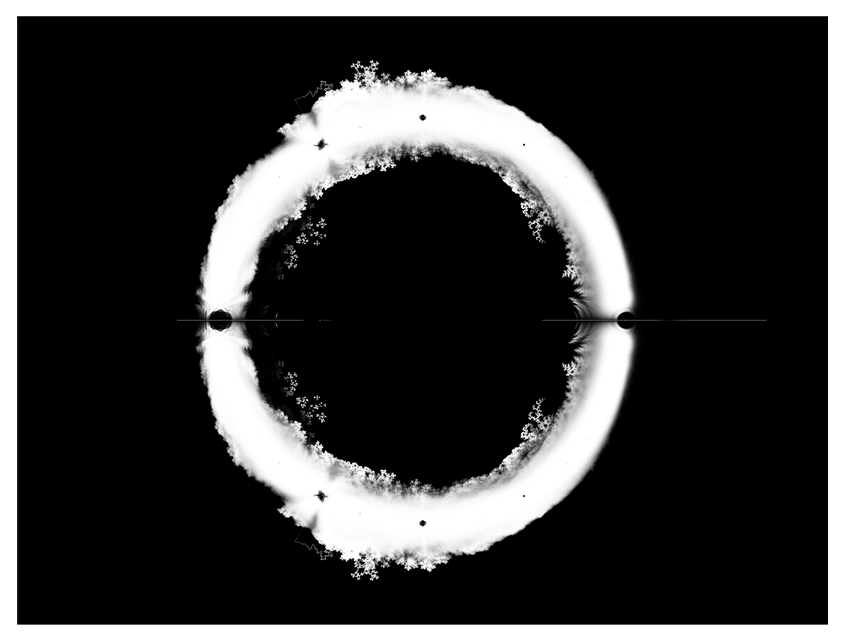
Figure 4. Galois conjugates of entropies of maps along the vein $v_{1/3}$.

Figure 5. Galois conjugates of entropies of maps along the vein $v_{1/5}$.

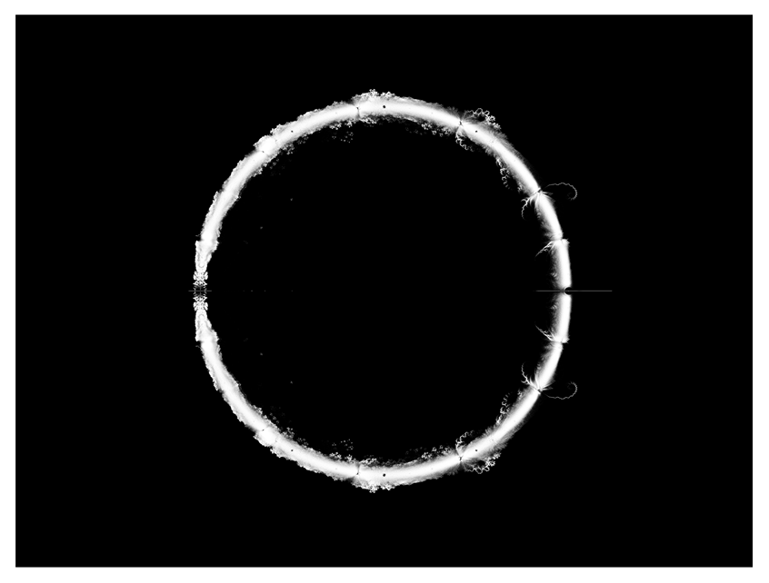
Figure 6. Galois conjugates of entropies of maps along the vein $v_{1/11}$.

References

- [B1] T. Bousch, Paires de similitudes Z SZ+1, Z SZ-1, preprint 1988.
- [B2] T. Bousch, Connexité locale et par chemins hölderiens pour les systèmes itérés de fonctions, preprint 1993.
- [Do1] A. Douady, Algorithms for computing angles in the Mandelbrot set, in Chaotic dynamics and fractals (Atlanta, Ga., 1985), Notes Rep. Math. Sci. Engrg. vol. 2, Academic Press, Orlando, FL, 1986.
- [Do2] A. Douady, Topological entropy of unimodal maps: monotonicity for quadratic polynomials, in “Real and complex dynamical systems (Hillerød, 1993)”, NATO Adv. Sci. Inst. Ser. C Math. Phys. Sci. 464, Kluwer, Dordrecht (1995), 65–87.
- [Ko] S.V. Konyagin, On the number of irreducible polynomials with coefficients, Acta Arith. 88 (1999), no. 4, 333–350.
- [MT] J. Milnor, W. Thurston, On iterated maps of the interval, Dynamical systems (College Park, MD, 1986–87), Lecture Notes in Math. 1342, 465–563, Springer, Berlin, 1988.
- [OP] A.M. Odlyzko, B. Poonen, Zeros of polynomials with coefficients, Enseign. Math. (2) 39 (1993), no. 3-4, 317–348.
- [Th] W. Thurston, Entropy in dimension one, preprint 2011.
- [Ti] G. Tiozzo, Topological entropy of quadratic polynomials and dimension of sections of the Mandelbrot set, arXiv:1305.3542 [math.DS].