Generation of distributed entangled coherent states over a lossy environment with inefficient detectors

Abstract

Entangled coherent states are useful for various applications in quantum information processing but they are are sensitive to loss. We propose a scheme to generate distributed entangled coherent states over a lossy environment in such a way that the fidelity is independent of the losses at detectors heralding the generation of the entanglement. We compare our scheme with a previous one for the same purpose [Ourjoumtsev et al., Nat. Phys. 5 189 (2009)] and find parameters for which our new scheme results in superior performance.

I Introduction

Entangled coherent states (ECSs) MecozziTombesi ; Sanders92 ; SandersReview are useful for various applications in quantum information processing vanEnkPRA2001 ; JeongPRA2001 ; Gerry2001 ; Wang2001 ; JeongPRA2002 ; JeongQIC2002 ; RalphPRA2003 ; An2003 ; JeongAn2006 ; LundPRL2008 ; AnKim2009 ; Munhoz2010 ; Joo2011 ; MyersRaph2011 ; Joo2012 ; Kirby2013 ; Jonas2013 and for exploring fundamental properties of quantum theory GerryGrobe1995 ; GerryGrobe1997 ; Wilson2002 ; JeongSon2003 ; Munro2000 ; Stobinska2007 ; JeongPRL2009 ; Paternostro2010 ; Lee2011 ; Tor2013 . An optical ECS can be generated by passing a single-mode superposition of coherent states (SCS) Milburn1985 ; YurkeStoler ; Schleich through a beam splitter. SCSs in free-traveling fields have been experimentally generated in several laboratories Ourjoumtsev2006 ; OurjoumtsevNature2007 ; SasakiPRL2008 ; Neer2010 ; Gerrits2010 . In order to use an ECS for quantum communication or faithful nonlocality tests, it should be distributed to two parties that are spatially separated. However, ECSs are sensitive to a lossy environment, a property typical of macroscopic entanglement. A method based on quantum repeaters for ECSs ECSrepeater may not be efficient due to the requirement of efficient photon-number-resolving detectors. It would thus be very useful to develop a scheme to efficiently generate an ECS distributed to two separate parties over a lossy environment.

Ourjoumtsev et al. experimentally demonstrated such a method for generating a distributed ECS grangier:nature . They utilized the fact that if an ECS is in an asymmetric form with different amplitudes for the two modes, the mode with the smaller amplitude is relatively more robust against loss. However, their approach grangier:nature is sensitive to inefficiency of the photon detector used for the necessary post-selection, and this formed a major part of the limitations in its practical applications.

In this paper, we present a scheme to generate distributed ECSs over a lossy environment whose output fidelities with ideal ECSs are insensitive to detection inefficiency. Our scheme employs the loss tolerant construction of Refs. JeongPRA2002 ; lund:catboost to achieve the robustness against lossy detection. We compare output fidelities obtained by our scheme with those of the previous one grangier:nature . We also show that there exists a range of parameters for which our scheme provides better results even when taking into account the lower success probability of the new scheme.

This paper is organized as follows. In Sec. II, we briefly review the loss tolerant detection for coherent state qubits JeongPRA2002 , which is employed as an important part in our scheme. In Sec. III, we review and analyze the scheme in Ref. grangier:nature . Our scheme is then presented in Sec. III with a comparison between the two proposals in terms of the success probabilities and the fidelities. We conclude our paper with final remarks in Sec. IV.

II Unambiguous and loss tolerant detection for coherent states

As a strategic part of our construction, we will first review unambiguous and loss tolerant detection for coherent state qubits discussed in Ref. JeongPRA2002 . This method was used for purifying ECSs JeongQIC2002 and amplifying SCSs lund:catboost . Suppose that one needs to unambiguously discriminate between two coherent states, $\ket{\pm\alpha}$ with amplitudes $\pm\alpha$, using two inefficient photon detectors. A simple way to perform this task is to apply a 50:50 beam splitter to interact the coherent state with an ancillary coherent state $\ket{\alpha}$ as shown in Fig. 1. If the input system mode was in state $|\alpha\rangle$, we get the transformation

$$\ket{\alpha,\alpha}\rightarrow\ket{\sqrt{2}\alpha,0},$$ (1)

and if the system was in state $\ket{-\alpha}$, the transformation is

$$\ket{-\alpha,\alpha}\rightarrow\ket{0,\sqrt{2}\alpha}.$$ (2)

This is an example of perfect classical interference and consequently only one of the two output modes contains any photons. It is then clear that only one of the two detectors in Fig. 1 can click for the final detection and such a click will unambiguously identify the initial state of the system. Of course, the signal we are trying to detect (i.e. $\ket{\pm\sqrt{2}\alpha}$) has a non-zero overlap with the vacuum state. This corresponds to the failure probability in which both the detectors are silent. It is important to note that inefficiency of the detectors will only increase this failure probability but it does not affect the unambiguous nature of the detection scheme. If we can ignore other experimental issues such as mode-mismatching at the beam splitter and dark counts at the detectors, the result will always be reliable as far as one of the detectors registers any photon(s).

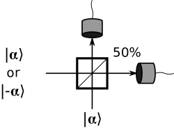
Figure 1: Loss tolerant detection scheme from Ref. JeongPRA2002 . A coherent state qubit encoded in the basis $\ket{\alpha}$ and $\ket{-\alpha}$ is interfered with a coherent state of the same amplitude at a 50:50 beam splitter. Perfect classical interference allows for the two input coherent states to be distinguished without error by recording which detector registers a click. However, due to the overlap of the two possible inputs, this measurement must be heralded and have some non-zero probability of failure. Failure occurs when no clicks are recorded. Detector loss increases this failure rate but does not induce errors in discrimination between the two basis states when photons are detected.

III Entanglement distribution using photon number detection

Writing the Bell basis in the form of ECSs gives

$$N_{\pm}(\sqrt{2}\alpha)\left(\ket{\alpha,\alpha}\pm\ket{-\alpha,-\alpha}\right),$$ (3)

where the other two Bell states are generated by applying a local $\pi$ phase shift to one mode. The task considered in this paper is generating a state of this form between two spatially separated parties that share a quantum channel, can perform local measurements and can communicate the results of these measurements via a classical channel.

Reference grangier:nature proposes and implements a method for generating distributed ECSs. The schematic for this scheme is shown in Fig. 2. The scheme requires two parties, here called A and B, to initially generate SCSs both with an encoding amplitude $\alpha^{\prime}$. Then both A and B use a beam-splitter to distribute a small fraction of energy $\epsilon$ from their SCS and send it to a central location C. To ensure that the entanglement generated has a particular coherent state encoding amplitude $\alpha$, it is necessary to set

$$\alpha^{\prime}=\sqrt{1+\epsilon^{\prime}}\alpha$$ (4)

where

$$\epsilon^{\prime}=\frac{\epsilon}{1+\epsilon}.$$ (5)

A loss of $\eta$ is present between A and C as well as B and C and it is an assumption of this analysis that losses are distributed evenly. This results in a total loss between A and B of

$$\eta_{T}=1-(1-\eta)^{2}.$$ (6)

At C the two low amplitude states are received and then interfered on a $50:50$ beam-splitter. Entanglement generation between A and B is heralded by the detection of a click at one of the outputs from the beam-splitter at C. Local corrections are applied by A and B depending on information C broadcasts about which mode a detection has been registered in and the detection outcome parity.

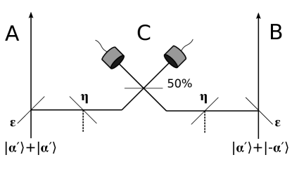
Figure 2: Entanglement distribution scheme from Ref. grangier:nature . A and B are the separated parties generating an ECS and C is a central herald. The parameters shown here are $\eta$ the one sided loss, $\epsilon$ the tapping off ratio and $\alpha^{\prime}$ defined in Eq. (4). These parameters are set so that the entanglement generated is a coherent state encoded Bell state with amplitude $\alpha$. Each detector has a loss of $l$ (not shown).

The probability of success and the fidelity with the ideal entangled coherent state can be computed and details of this calculation are shown in Appendix A. To simplify the expressions a little we write

$$\eta^{\prime}=\sqrt{\eta}+l-l\sqrt{\eta}$$ (7)

where $l$ is the detector loss. Having these parameters combine like this is expected as the scheme treats detector loss and channel loss similarly due to the symmetry of the losses and the linear beam-splitter interaction. We split the probability and fidelity expressions into the two cases of the herald detecting an even and odd number of photons in one detector. The expressions for fidelity and probability of generation are

$$\mathcal{F}_{even}=(1+\tanh(2\epsilon^{\prime}\eta^{\prime}\alpha^{2})\tanh(2\alpha^{2}))^{-1}$$ (8)

$$P_{even}=\frac{e^{-2\epsilon^{\prime}\alpha^{2}}}{(1+e^{-2(1+\epsilon^{\prime})\alpha^{2}})}\left(\cosh(2\epsilon^{\prime}(1-\eta^{\prime})\alpha^{2})-1\right)\left(\cosh(2\epsilon^{\prime}\eta^{\prime}\alpha^{2})(1+e^{-2\alpha^{2}})+\sinh(2\epsilon^{\prime}\eta^{\prime}\alpha^{2})(1-e^{-2\alpha^{2}})\right)$$ (9)

$$\mathcal{F}_{odd}=(1+\tanh(2\epsilon^{\prime}\eta^{\prime}\alpha^{2})\coth(2\alpha^{2}))^{-1}$$ (10)

$$P_{odd}=\frac{e^{-2\epsilon^{\prime}\alpha^{2}}}{(1+e^{-2(1+\epsilon^{\prime})\alpha^{2}})}\sinh(2\epsilon^{\prime}(1-\eta^{\prime})\alpha^{2})\left(\sinh(2\epsilon^{\prime}\eta^{\prime}\alpha^{2})(1+e^{-2\alpha^{2}})+\cosh(2\epsilon^{\prime}\eta^{\prime}\alpha^{2})(1-e^{-2\alpha^{2}})\right)$$ (11)

where for each probability we have summed over the two possibilities of which detector measures the photons and the output state is assumed to have had any local phase shift correction applied.

The key idea for this scheme which builds resilience to channel loss is that the energy distributed is small and hence the chance of loosing a quanta of energy is also small. For each quanta of energy lost a sign flip ($Z$) error is introduced in the coherent-state basis, therefore if $\epsilon$ is small the error rate can be low. This can be seen in the fidelity equations by allowing $\epsilon\ll\alpha^{2}$ and $\epsilon\ll l^{\prime}\alpha^{2}$. However, under these conditions, the probability of getting the heralding signal is also small. These losses can be a roadblock to implementing scaled-up protocols ECSrepeater .

IV Proposed scheme with realistic on/off detectors

We will now construct a new scheme which uses the loss tolerant unambiguous state discrimination as a herald and maintains the feature of distributing a very low amplitude through the lossy channel.

The two parties A and B, generate SCSs as before but of different amplitude as this new protocol is asymmetric between the two parties. Here A is the sender. Party A generates a cat-state state of amplitude $\sqrt{1+\epsilon^{\prime}}\alpha$ and sends a proportion $\epsilon$ along the lossy channel $\eta_{T}$ to the receiving party B. Party B then combines the small received amplitude with a cat-state state of amplitude

$$\alpha^{\prime\prime}=\sqrt{\rho}\alpha$$ (12)

on a beam-splitter with reflectivity $\rho$ where

$$\rho=\epsilon^{\prime}(1-\eta_{T}).$$ (13)

The heralding is performed by B who takes one of the output modes of the beam-splitter mixes that with a coherent state of amplitude $\sqrt{\gamma}\alpha$ where

$$\gamma=4\rho(1-\rho).$$ (14)

All of these parameters are chosen so that the final output that A and B will share is an ECS with encoding amplitude $\alpha$ and so that for the states where the coherent state phases A and B share are the same, the state input into the detector at B is the vacuum state. There are only three free variables which determine all parameters at this point, $\alpha$, $\epsilon$ and $\eta_{T}$. Successful entanglement generation is heralded when a detection occurs (of any non-zero number of photons) in one of the two outputs from this final beam-splitter with detector losses of $l$. Note that there is now no central party which acts as a herald as this is done by the receiver B who must communicate to A which events were successful. The successful output state is an ECS with a positive superposition and in phase coherent states. This is the same state produced with the previous scheme on achieving an even parity success result.

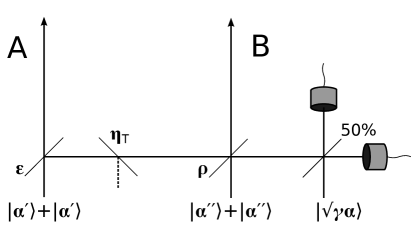
Figure 3: Our proposed entanglement distribution scheme. The parameters $\alpha^{\prime}$ and $\eta_{T}$ are the same as before and defined in Eqs. (4) and (6). New parameters $\alpha^{\prime\prime}$, $\rho$ and $\gamma$ are defined in Eqs. (12), (13) and (14). Just as before each detector has a loss of $l$ and the encoding of the heralded ECS is $\alpha$. This scheme only has one success signal and on achieving it an ECS with a positive superposition and in phase coherent states is produced.

Figure 4: Fidelity (top curves, LHS axis) and probability of success (bottom curves, RHS axis) as a function of the output encoding coherent state amplitude $\alpha$. Parameters used for these plots are $\epsilon=0.1$, $\eta_{T}=0.5$, $l=0.5$. ‘Odd’ and ‘even’ refer to the scheme from grangier:nature when the post-selection is done by counting an odd number of photons or an even but non-zero number of photons respectively. ‘New’ refers to the new scheme presented here.

The fidelity of this new scheme is given by

$$\mathcal{F}_{new}(\alpha)=\frac{1}{(1+\tanh(\epsilon\eta_{T}\alpha^{2})\tanh(2(1-\epsilon)\alpha^{2}))}$$ (15)

and the probability of success

$$P_{new}(\alpha)=\frac{(1-\exp(-(1-l)\gamma^{2}/2))^{2}}{2(1+\cosh((1-\rho)\alpha^{2})/\cosh((1+\rho)\alpha^{2}))}.$$ (16)

The details of this calculation are similar to that which were performed for the other scheme and are contained in Appendix B. Figure 4 compares these new values for fidelity and probability against those computed for the previous scheme using the same channel and detector parameters. This plot shows that for a fixed channel loss the fidelity of achieving the desired coherent state size is higher for all amplitudes when using the new scheme. However, the probability is lower than the probabilities of success for the old scheme.

Figure 5: Parametric plot of fidelity and probability using coherent state amplitude as the parameter. This plot was generated for $\epsilon=0.1$, $\eta=0.5$ and $l=0.5$ as in Fig. 4. For the low probability events, which correspond to smaller choices of $\alpha$ we see that the new scheme has a region in which it is better in both probability and fidelity for this choice of parameters. For the choice of parameters in this plot, the region of higher probability and fidelity of our new scheme is for $\alpha\lessapprox 1.2$.

If the encoding amplitude of the output entangled state is not required to be a particular value, then this suggests a trade off would be possible between fidelity and probability. To make this comparison we plot in Fig. 5 a parametric plot of fidelity and probability where the parameter defining the curve is $\alpha$. Under this relaxed comparison we can see that there is a region when the encoding size is small in which for a given probability of success the fidelity of the new scheme is superior.

V Conclusion

We have proposed and analysed a scheme for generating entangled coherent states over a lossy environment which utilises a loss tolerant unambiguous detection scheme to perform the heralding measurement. We have compared this scheme to one designed for a similar purpose in Ref. grangier:nature which uses photon number resolving detectors for heralding. We find that for any given coherent state encoding amplitude, our scheme gives a better fidelity, but a lower probability of success. However, if comparison is made where the encoding amplitude is not required to be the same, we find that for a given probability of success our scheme can give a higher fidelity. In particular, when channel loss and detector loss are both $50\%$, a better fidelity for the same probability is possible with our new scheme when preparing an ECS with $\alpha\lessapprox 1.2$. Our study may be useful for long-distance quantum communication using SCSs and realistic detectors.

Appendix A Analysis of Ourjoumtsev et al.’s Scheme

We here present a detailed analysis of the scheme in Ref. grangier:nature to find the fidelity and the success probability. The methodology for the calculation is quite simple, however the equations that result can be long and difficult to work with. There are three steps to the process. First SCSs are prepared. Next the prepared states are evolved in a linear optical network. Finally, some of the output modes are detected. The calculation we wish to perform is to find the output state from the modes which are not detected conditional on the particular results from the measured modes.

The output state, including the amplitude and phase terms, for each coherent states which make up the basis states in the coherent state superposition are calculated. Then to calculate the output state for the input coherent state superposition, the terms are added together. The probability can then be computed as the normalisation of this resultant state. The fidelity can then be calculated by computing the overlap between renormalised state and the desired entangled coherent state superposition.

The evolution of coherent states through a linear optical network is exactly that which would result from the classical field amplitudes with the coherent state eigenvalue playing the role of the field amplitude. The evolution on the coherent state basis states for the scheme from grangier:nature can be calculated from the schematic shown in Fig. 2. This linear network with loss $\eta$ on both halfs of the channel and detector loss $l$, induces the transformation on the coherent states as

$$\ket{\pm\sqrt{1+\epsilon^{\prime}}\alpha,\pm\sqrt{1+\epsilon^{\prime}}\alpha}\rightarrow\ket{\pm\alpha,\pm\alpha,\pm\sqrt{2\epsilon^{\prime}(1-\eta)(1-l)}\alpha,0,\underline{\pm\sqrt{\epsilon^{\prime}\eta}\alpha},\underline{\pm\sqrt{\epsilon^{\prime}\eta}\alpha},\underline{\pm\sqrt{2\epsilon^{\prime}(1-\eta)l}\alpha},\underline{0}},$$

$$\ket{\pm\sqrt{1+\epsilon^{\prime}}\alpha,\mp\sqrt{1+\epsilon^{\prime}}\alpha}\rightarrow\ket{\pm\alpha,\mp\alpha,0,\pm\sqrt{2\epsilon^{\prime}(1-\eta)(1-l)}\alpha,\underline{\pm\sqrt{\epsilon^{\prime}\eta}\alpha},\underline{\mp\sqrt{\epsilon^{\prime}\eta}\alpha},\underline{0},\underline{\pm\sqrt{2\epsilon^{\prime}(1-\eta)l}\alpha}}.$$

where

$$\epsilon^{\prime}=\frac{\epsilon}{1-\epsilon}$$

and $\epsilon$ is the initial tapping off ratio. On the right hand side of the equation we have chosen the ordering of modes to be: A output, B output, C output 1 (detected), C output 2 (detected), A channel loss mode, B channel loss mode, C detector loss 1, C detector loss 2. Detector modes will be projected onto the Fock basis state corresponding to the detection results and the loss modes, shown underlined, will be traced out.

C detects $n$ and $m$ in the detector outputs and $a$,$b$,$c$,$d$ photons are present in the environment (which will eventually be summed over to perform the trace), then we have the transformation including the amplitude and phase factors

$$\ket{\sqrt{1+\epsilon^{\prime}}\alpha,\sqrt{1+\epsilon^{\prime}}\alpha}\rightarrow e^{-\epsilon^{\prime}\alpha^{2}}\frac{\left(\sqrt{2\epsilon^{\prime}(1-\eta)(1-l)}\alpha\right)^{n}}{\sqrt{n!}}\delta_{m,0}\frac{\left(\sqrt{\epsilon^{\prime}\eta}\alpha\right)^{a+b}}{\sqrt{a!b!}}\frac{\left(\sqrt{2(1-\eta)\epsilon^{\prime}l}\alpha\right)^{c}}{\sqrt{c!}}\delta_{d,0}\ket{\alpha,\alpha},$$

$$\ket{-\sqrt{1+\epsilon^{\prime}}\alpha,-\sqrt{1+\epsilon^{\prime}}\alpha}\rightarrow e^{-\epsilon^{\prime}\alpha^{2}}\frac{\left(\sqrt{2\epsilon^{\prime}(1-\eta)(1-l)}\alpha\right)^{n}}{\sqrt{n!}}(-1)^{n}\delta_{m,0}\frac{\left(\sqrt{\epsilon^{\prime}\eta}\alpha\right)^{a+b}}{\sqrt{a!b!}}(-1)^{a+b}\frac{\left(\sqrt{2\epsilon^{\prime}(1-\eta)l}\alpha\right)^{c}}{\sqrt{c!}}(-1)^{c}\delta_{d,0}\ket{-\alpha,-\alpha},$$

$$\ket{\sqrt{1+\epsilon^{\prime}}\alpha,-\sqrt{1+\epsilon^{\prime}}\alpha}\rightarrow e^{-\epsilon^{\prime}\alpha^{2}}\delta_{n,0}\frac{\left(\sqrt{2\epsilon^{\prime}(1-\eta)(1-l)}\alpha\right)^{m}}{\sqrt{m!}}\frac{\left(\sqrt{\epsilon^{\prime}\eta}\alpha\right)^{a+b}}{\sqrt{a!b!}}(-1)^{b}\delta_{c,0}\frac{\left(\sqrt{2\epsilon^{\prime}(1-\eta)l}\alpha\right)^{d}}{\sqrt{d!}}\ket{\alpha,-\alpha},$$

$$\ket{-\sqrt{1+\epsilon^{\prime}}\alpha,\sqrt{1+\epsilon^{\prime}}\alpha}\rightarrow e^{-\epsilon^{\prime}\alpha^{2}}\delta_{n,0}\frac{\left(\sqrt{2\epsilon^{\prime}(1-\eta)(1-l)}\alpha\right)^{m}}{\sqrt{m!}}(-1)^{m}\frac{\left(\sqrt{\epsilon^{\prime}\eta}\alpha\right)^{a+b}}{\sqrt{a!b!}}(-1)^{a}\delta_{c,0}\frac{\left(\sqrt{2\epsilon^{\prime}(1-\eta)l}\alpha\right)^{d}}{\sqrt{d!}}(-1)^{d}\ket{\alpha,-\alpha},$$

where $\delta_{x,y}$ is the Kronecker delta. Now we can use linearity of the evolution of the quantum state to compute the output given an input which is a superposition of these coherent state inputs. The normalized input state is

$$N_{+}(\sqrt{1+\epsilon^{\prime}}\alpha)^{2}\left(\ket{\sqrt{1+\epsilon^{\prime}}\alpha}+\ket{-\sqrt{1+\epsilon^{\prime}}\alpha}\right)\otimes\left(\ket{\sqrt{1+\epsilon^{\prime}}\alpha}+\ket{-\sqrt{1+\epsilon^{\prime}}\alpha}\right)=\\ N_{+}(\sqrt{1+\epsilon^{\prime}}\alpha)^{2}\left(\ket{\sqrt{1+\epsilon^{\prime}}\alpha,\sqrt{1+\epsilon^{\prime}}\alpha}+\ket{-\sqrt{1+\epsilon^{\prime}}\alpha,\sqrt{1+\epsilon^{\prime}}\alpha}+\ket{\sqrt{1+\epsilon^{\prime}}\alpha,-\sqrt{1+\epsilon^{\prime}}\alpha}+\ket{-\sqrt{1+\epsilon^{\prime}}\alpha,-\sqrt{1+\epsilon^{\prime}}\alpha}\right)$$ (17)

where

$$N_{\pm}(\beta)=\frac{1}{\sqrt{2(1\pm e^{-2\beta^{2}})}}$$

to which we then need to apply the above transformations. We can see that this results in the superposition of all of the above transformations.

This would result in a very long expression for the output state. However, we can look at particular values of the heralding signal to pick apart the components. If we consider the case where $m=0$ and $n\neq 0$ then the output which results from the input components $\ket{\sqrt{1+\epsilon^{\prime}}\alpha,-\sqrt{1+\epsilon^{\prime}}\alpha}$ and $\ket{-\sqrt{1+\epsilon^{\prime}}\alpha,\sqrt{1+\epsilon^{\prime}}\alpha}$ have zero contribution to the output state. This is due to the coherent state amplitude at the detector corresponding to the $n$ mode being zero. Therefore for this case we only need consider the top two transformations. If we consider the case where $n$ is odd and consider the traced out modes to be measured in the Fock basis (this choice is arbitrary, as the trace is basis independent, but convenient) then we find the output state is then

$$N_{+}(\sqrt{1-\epsilon^{\prime}}\alpha)^{2}e^{-\epsilon^{\prime}\alpha^{2}}\frac{\left(\alpha\sqrt{2\epsilon^{\prime}(1-\eta)(1-l)}\right)^{n}}{\sqrt{n!}}\frac{\left(\alpha\sqrt{\epsilon^{\prime}\eta}\right)^{a+b}}{\sqrt{a!b!}}\frac{\left(\alpha\sqrt{2\epsilon^{\prime}(1-\eta)l}\right)^{c}}{\sqrt{c!}}\delta_{d,0}\ket{(-1)^{a+b+c+1}\ _{\alpha}}$$

where

$$\ket{\pm_{\beta}}=\ket{\beta,\beta}\pm\ket{-\beta,-\beta}$$

and is unnormalised. The sign of the superposition is determined by the numbers $a$,$b$ and $c$ which relate to the number of photons in the loss modes. We need to mix over these possibilities to complete the partial trace. Each sum can be computed individually. Take for example the sum over $c$. There are two cases, where $c$ is odd and where $c$ is even (including zero). When it is even, the $\ket{-\alpha,-\alpha}$ state contributes no minus sign relative to the $\ket{\alpha,\alpha}$ state and the output state is the same for all even cases, though the amplitude is different. When it is odd, there is a sign change, but again the state is the same for all odd cases. When the sum is performed the coefficients sum to a hyperbolic function. This same effect will occur for the $a$ and $b$ summations as well. The sign changes can be combined as two minus signs cancel.

Applying these sums and the hyperbolic trigonometric double angle formula, results in the output state

$$N_{+}(\sqrt{1+\epsilon^{\prime}}\alpha)^{4}e^{-2\epsilon^{\prime}\alpha^{2}}\frac{(2\epsilon^{\prime}(1-\eta^{\prime})\alpha^{2})^{n}}{n!}\left(\sinh(2\epsilon^{\prime}\eta^{\prime}\alpha^{2})\ket{+_{\alpha}}\bra{+_{\alpha}}+\cosh(2\epsilon^{\prime}\eta^{\prime}\alpha^{2})\ket{-_{\alpha}}\bra{-_{\alpha}}\right)$$

where

$$\eta^{\prime}=1-(1-l)\sqrt{1-\eta_{T}}$$ (18)

where $\eta_{T}$ is the total loss between the two parties. The number $\eta^{\prime}$ is the combination of half the channel loss and loss from one of the detectors. Note that when $m$ is odd and $n=0$ we obtain the same formula for the even case if one of the modes is phase shifted by $\pi$ as merely the other two components of the input state are selected out. This results in effectively multiplying the even and odd case density operators by two. Finally, for the even case that the result will be an expression of the same form but with the minus and plus states swapped. The only case in which an expression like this is not applicable is when $m=0$ and $n=0$. We can now sum over those states where the output is identical and assume that the easy phase shift correction has been applied (but not to the superposition sign change) to result in two expressions, one for the case of an even (but non-zero) result

$$\rho_{even}=N_{+}(\sqrt{1+\epsilon^{\prime}}\alpha)^{4}e^{-2\epsilon^{\prime}\alpha^{2}}(\cosh(2\epsilon^{\prime}(1-\eta^{\prime})\alpha^{2})-1)\left(\cosh(2\epsilon^{\prime}\eta^{\prime}\alpha^{2})\ket{+_{\alpha}}\bra{+_{\alpha}}+\sinh(2\epsilon^{\prime}\eta^{\prime}\alpha^{2})\ket{-_{\alpha}}\bra{-_{\alpha}}\right)$$ (19)

and for the odd result

$$\rho_{odd}=N_{+}(\sqrt{1+\epsilon^{\prime}}\alpha)^{4}e^{-2\epsilon^{\prime}\alpha^{2}}\sinh(2\epsilon^{\prime}(1-\eta^{\prime})\alpha^{2})\left(\sinh(2\epsilon^{\prime}\eta^{\prime}\alpha^{2})\ket{+_{\alpha}}\bra{+_{\alpha}}+\cosh(2\epsilon^{\prime}\eta^{\prime}\alpha^{2})\ket{-_{\alpha}}\bra{-_{\alpha}}\right).$$ (20)

It is important to note that in the notation used here the plus and the minus kets are unnormalised entangled states. To calculate probability and fidelity it is important to keep this in mind or factor out a normalisation coefficient which will in general not be $1/\sqrt{2}$ do to the overlap of the states forming the superposition. So from these expressions we obtain the probabilities of success in Eqs. (9) and (11) from the trace and the fidelities in Eqs. (8) and (10) are calculated by using the probabilities of success to renormalise the density operator, then take the appropriate coefficients (the minus superposition for odd and plus superposition for even).

Appendix B Proposed Scheme

The calculation of the fidelity and probability for the scheme proposed in this paper proceeds in much the same way as that given above. First we write down the transformation of the basis coherent states through the linear network including the lossy channel.

$$\ket{\pm\sqrt{1+\epsilon^{\prime}}\alpha,\pm\sqrt{1-\rho}\alpha,\sqrt{\gamma}\alpha}\rightarrow\ket{\pm\alpha,\pm\alpha,\underline{\pm\sqrt{\epsilon^{\prime}\eta_{T}}\alpha},\sqrt{\frac{\gamma}{2}}\alpha,\sqrt{\frac{\gamma}{2}}\alpha}$$

$$\ket{\pm\sqrt{1+\epsilon^{\prime}}\alpha,\mp\sqrt{1-\rho}\alpha,\sqrt{\gamma}\alpha}\rightarrow\ket{\pm\alpha,\pm 2\rho\alpha,\underline{\pm\sqrt{\epsilon^{\prime}\eta_{T}}\alpha},\begin{array}[]{cc}0\\ \sqrt{2}\gamma\end{array},\begin{array}[]{cc}\sqrt{2}\gamma\\ 0\end{array}}$$

where

$$\rho=\epsilon^{\prime}(1-\eta_{T})$$

which is also the reflectivity of the beamsplitter for side B and

$$\gamma=4\rho(1-\rho).$$

The mode ordering on the right hand side is: A output, B output, channel loss, B detector 1, B detector 2. The channel loss mode is underlined as it is to be traced out. The mode ordering on the left hand side is: A input, B input and B detector input. There are input modes associated with the loss mode and with the beam-splitter with A which are always prepared in the vacuum state and are not shown. In the case where the signs of the input coherent states are the same, perfect interference occurs before the unambiguous state discrimination scheme and results in the vacuum being input, hence the coherent state splits evenly and with the same sign. This occurs by design and is why the parameters take the values given above. In the other two cases the input is either the plus or minus $\gamma$ coherent state and hence the usual situation for the unambiguous state discrimination applies.

These transformations are then applied to the input SCS states

$$N_{+}(\sqrt{1+\epsilon^{\prime}}\alpha)N_{+}(\sqrt{1-\rho}\alpha)(\ket{\sqrt{1+\epsilon^{\prime}}\alpha}+\ket{-\sqrt{1+\epsilon^{\prime}}\alpha})\otimes(\ket{\sqrt{1-\rho}\alpha}+\ket{\sqrt{1-\rho}\alpha})=\\ N_{+}(\sqrt{1+\epsilon^{\prime}}\alpha)N_{+}(\sqrt{1-\rho}\alpha)\left(\ket{\sqrt{1+\epsilon^{\prime}}\alpha,\sqrt{1-\rho}\alpha}+\ket{\sqrt{1+\epsilon^{\prime}}\alpha,-\sqrt{1-\rho}\alpha}\right.\\ \left.+\ket{-\sqrt{1+\epsilon^{\prime}}\alpha,\sqrt{1-\rho}\alpha}+\ket{-\sqrt{1+\epsilon^{\prime}}\alpha,-\sqrt{1-\rho}\alpha}\right).$$ (21)

Successful detection occurs when both of the detectors record a click of any number of photons. This will clearly select out the cases where the sign of the coherent state in both A and B’s output is the same. Proceeding as before we will compute the partial trace in the Fock basis. So, if $a$ photons are in the loss mode and the detectors register $n\neq 0$ and $m\neq 0$ photons the output state is

$$N_{+}(\sqrt{1+\epsilon^{\prime}}\alpha)N_{+}(\sqrt{1-\rho}\alpha)e^{-(\eta_{T}\epsilon^{\prime}+\gamma)\alpha^{2}/2}\frac{1}{\sqrt{n!m!}}\left(\sqrt{\frac{\gamma}{2}}\alpha\right)^{n+m}\frac{(\sqrt{\eta_{T}\epsilon^{\prime}}\alpha)^{a}}{\sqrt{a!}}\ket{{(-1)^{a}}_{\alpha}}.$$

The reduced density matrix when tracing out $a$ is

$$N_{+}(\sqrt{1+\epsilon^{\prime}}\alpha)^{2}N_{+}(\sqrt{1-\rho}\alpha)^{2}(1-e^{-\gamma\alpha^{2}/2})^{2}e^{-\eta_{T}\epsilon^{\prime}\alpha^{2}}\left(\cosh(\eta_{T}\epsilon^{\prime}\alpha^{2})\ket{+_{\alpha}}\bra{+_{\alpha}}+\sinh(\eta_{T}\epsilon^{\prime}\alpha^{2})\ket{-_{\alpha}}\bra{-_{\alpha}}\right)$$

that we obtain the success probability and fidelity in Eqs. (15) and (16). Incorporating detector loss for the success case is simply a matter of reducing the coherent state amplitude by a factor of $\sqrt{1-l}$ as the state incident upon the detector is a coherent state and loss will merely reduce the coherent state amplitude and no superpositions of coherent states occur when a successful signal is achieved. This can be achieved by adjusting $\gamma$ so that it is $\sqrt{1-l}$ times smaller. This then recreates equation 14. Here we can see that the fidelity is independent of $\gamma$, one of the critical features of our design.

References

- (1) A. Mecozzi and P. Tombesi, Phys. Rev. Lett. 58, 1055 (1987).
- (2) B. C. Sanders, Phys. Rev. A 45, 6811 (1992).
- (3) B. C. Sanders, J. Phys. A 45, 244002 (2012).
- (4) S. J. van Enk and O. Hirota, Phys. Rev. A 64, 022313 (2001).
- (5) H. Jeong, M. S. Kim, and J. Lee, Phys. Rev. A 64, 052308 (2001).
- (6) X. Wang, Phys. Rev. A 64, 022302 (2001).
- (7) C. C. Gerry, and R. A. Campos, Phys. Rev. A 64, 063814 (2001).
- (8) H. Jeong and M. S. Kim, Phys. Rev. A 65, 042305 (2002).
- (9) H. Jeong and M. S. Kim, Quantum Information and Computation 2, 208 (2002).
- (10) T. C. Ralph, A. Gilchrist, G. J. Milburn, W. J. Munro, and S. Glancy, Phys. Rev. A. 68, 042319 (2003).
- (11) N. B. An, Phys. Rev. A 68, 022321 (2003).
- (12) H. Jeong and N. B. An, Phys. Rev. A 74, 022104 (2006).
- (13) A. P. Lund, T. C. Ralph, and H. L. Haselgrove, Phys. Rev. Lett. 100, 030503 (2008).
- (14) N. B. An and J. Kim, Phys. Rev. A 80, 042316 (2009).
- (15) P. P. Munhoz, J. A. Roversi, A. Vidiella-Barranco, and F. L. Semião, Phys. Rev. A 81, 042305 (2010).
- (16) J. Joo, W. J. Munro, and T. P. Spiller, Phys. Rev. Lett. 107, 083601 (2011).
- (17) C. R. Myers and T. C. Ralph, New J. Phys. 13, 115015 (2011).
- (18) J. Joo, K. Park, H. Jeong, W. J. Munro, K. Nemoto, and T. P. Spiller, Phys. Rev. A 86, 043828 (2012).
- (19) B. T. Kirby and J. D. Franson, Phys. Rev. A 87, 053822 (2013); B. T. Kirby and J. D. Franson, arXiv:1310.1846.
- (20) J. S. Neergaard-Nielsen, Y. Eto, C.-W. Lee, H. Jeong, and M. Sasaki, Nat. Photonics 7, 439 (2013).
- (21) C. C. Gerry and R. Grobe, Phys. Rev. A 51, 1698 (1995).
- (22) C. C. Gerry and R. Grobe, Phys. Rev. A 75, 034303 (2007).
- (23) W. J. Munro, G. J. Milburn, and B. C. Sanders, Phys. Rev. A 62, 052108 (2000).
- (24) D. Wilson, H. Jeong, and M. S. Kim, Journal of Modern Optics 49, 851 (2002).
- (25) H. Jeong, W. Son, M. S. Kim, D. Ahn, and C. Brukner, Phys. Rev. A 67, 012106 (2003).
- (26) M. Stobinska, H. Jeong, and T. C. Ralph, Phys. Rev. A 75, 052105 (2007).
- (27) H. Jeong, M. Paternostro, and T. C. Ralph, Phys. Rev. Lett. 102, 060403 (2009).
- (28) M. Paternostro and H. Jeong, Phys. Rev. A 81, 032115 (2010).
- (29) C.-W. Lee, M. Paternostro, and H. Jeong, Phys. Rev. A 83, 022102 (2011).
- (30) G. Torlai, G. McKeown, P. Marek, R. Filip, H. Jeong, M. Paternostro, and G. De Chiara, Phys. Rev. A 87, 052112 (2013).
- (31) G. J. Milburn, Phys. Rev. A 33, 674 (1985).
- (32) B. Yurke and D. Stoler, Phys. Rev. Lett. 57, 13 (1986).
- (33) W. Schleich, M. Pernigo, and F.L. Kien, Phys. Rev. A 44, 2172 (1991).
- (34) A. Ourjoumtsev, R. Tualle-Brouri, J. Laurat, and P. Grangier, Nature 448, 784 (2007).
- (35) A. Ourjoumtsev, H. Jeong, R. Tualle-Brouri and P. Grangier, Nature 448, 784 (2007).
- (36) H. Takahashi, K. Wakui, S. Suzuki, M. Takeoka, K. Hayasaka, A. Furusawa, and M. Sasaki, Phys. Rev. Lett. 101, 233605 (2008).
- (37) J. S. Neergaard-Nielsen, M. Takeuchi, K. Wakui, H. Takahashi, K. Hayasaka, M. Takeoka, and M. Sasaki, Phys. Rev. Lett. 105, 053602 (2010).
- (38) T. Gerrits, S. Glancy, T. S. Clement, B. Calkins, A. E. Lita, A. J. Miller, A. L. Migdall, S. W. Nam, R. P. Mirin, and E. Knill, Phys. Rev. A 82, 031802(R) (2010).
- (39) N. Sangouard, C. Simon, N. Gisin, J. Laurat, R. Tualle-Brouri, and Ph. Grangier, J. Opt. Soc. Am. B 27, A137 (2010).
- (40) A. Ourjoumtsev, F. Ferreyrol, R. Tualle-Brouri, and P. Grangier, Nature Physics 5, 189 (2009).
- (41) A. P. Lund, H. Jeong, T. C. Ralph, and M. S. Kim, Phys. Rev. A 70, 020101 (2004).