Nonlinear $\mathcal{PT}$-Symmetric models Bearing Exact Solutions

Abstract

We study the nonlinear Schrödinger equation with a ${\cal PT}$-symmetric potential. Using a hydrodynamic formulation and connecting the phase gradient to the field amplitude, allows for a reduction of the model to a Duffing or a generalized Duffing equation. This way, we can obtain exact soliton solutions existing in the presence of suitable ${\cal PT}$-symmetric potentials, and study their stability and dynamics. We report interesting new features, including oscillatory instabilities of solitons and (nonlinear) ${\cal PT}$-symmetry breaking transitions, for focusing and defocusing nonlinearities.

1 Introduction

It is well known that in quantum mechanics the energy spectrum, as well as the spectrum of operators associated with observables, is real. This led to the commonly adopted assumption that the Hamiltonian $\hat{H}$ must be Hermitian, which guarantees a real spectrum. However, non-hermitian Hamiltonians respecting $\mathcal{P}\mathcal{T}$-symmetry, can also present entirely real spectra (within suitable parametric ranges) [1, 2]. The parity operator $\mathcal{P}$ corresponds to spatial reflections, $\hat{p}\to-\hat{p}$ and $\hat{x}\to-\hat{x}$, while the time reversal operator $\mathcal{T}$ corresponds to $\hat{p}\to-\hat{p}$, $\hat{x}\to\hat{x}$ and $i\to-i$.

While the subject of $\mathcal{P}\mathcal{T}$-symmetric systems was initially studied in the context of quantum mechanics, relevant experimental realizations emerged in other fields, most notably in optics. In particular, such systems were proposed [3, 4, 5, 6, 7] and subsequently experimentally implemented [8, 9] in systems of optical waveguides. Another physical context where such systems have been experimentally “engineered” is that of electronic circuits [10, 11]. Recently, experiments on $\mathcal{P}\mathcal{T}$-symmetric media have also appeared in the context of whispering gallery modes[12]. In parallel to these significant experimental developments, there has been an ever expanding volume of theoretical works, considering both continuum and discrete models (see, e.g., the recent review [13] and references therein). Given the spatial limitations of this contribution, we do not summarize these works here, but rather focus on efforts relevant to the considerations herein.

Already from the early works studying the interplay between ${\cal PT}$-symmetry and nonlinearity [4, 5], it became apparent that exact solutions could be analytically obtained for suitably “carved” potentials —such as the Scarff-II potential [14]. The idea of using Rosen-Morse type ${\cal PT}$-symmetric potentials, and obtaining analytical solutions thereof, was recently generalized to multiple potential parameters and higher-dimensional cases in Ref. [15]. More recently, the relevant approach was revisited and generalized [16], using a decomposition into amplitude and phase, for a ${\cal PT}$-symmetric term also in the nonlinear part of the equation; the emphasis was on producing an effective equation for the density, with either a parabolic confining potential or to construct effective equations with elliptic function potentials, which support exact analytical solutions. Notice that the considerations in the latter case, were driven by the form of the real part of the potential.

Here, we consider a system with a $\mathcal{P}\mathcal{T}$-symmetric Hamiltonian, namely a one-dimensional (1D) nonlinear Schrödinger (NLS) equation with a complex potential:

$$iu_{t}=-\frac{1}{2}u_{xx}+\sigma|u|^{2}u+[V(x)+iW(x)]u,$$ (1)

where $u$ is a complex field, subscripts denote partial derivatives, $\sigma=+1$ ($\sigma=-1$) corresponds to a defocusing (focusing) nonlinearity, while $V(x)$ and $W(x)$ correspond, respectively, to the real and imaginary (i.e., gain/loss) parts of the external potential. Note that the system possesses a ${\cal PT}$-symmetric Hamiltonian if $V(x)$ and $W(x)$ are, respectively, even and odd functions of $x$. Our aim is to return to the ideas of Refs. [15, 16], but from a different perspective. On the one hand, regarding the existence problem, we consider cases with $V(x)=0$, connecting the problem with the Duffing equation or generalizations thereof (involving also higher exponents). On the other hand, we also place some emphasis on the stability analysis of the obtained solutions, both for $\sigma=\pm 1$. Particularly, we present some interesting features including the (unusual) emergence of oscillatory instabilities for single bright solitons, or the existence of a nonlinear ${\cal PT}$-phase transition between the homogeneous and the dark soliton state for defocusing cubic-quintic nonlinearities. For all the obtained solutions, upon exploring their existence and stability, numerical simulations are developed to appreciate their dynamical evolution.

Our presentation is structured as follows. In section II, we focus on analytical considerations of the existence problem, providing a systematic approach for generalized Duffing functional forms. In section III, we explore some case examples of focusing and defocusing cubic and cubic-quintic cases. Finally, in section IV, we summarize our findings and present some future challenges.

2 Theoretical Setup

We seek stationary solutions to Eq. (1) in the form $u=\rho(x)\exp[i\phi(x)-i\mu t]$, where the amplitude $\rho(x)$ and phase $\phi(x)$ are real-valued functions. The resulting hydrodynamic-type equations for $\rho(x)$ and $\phi$ read:

$$\rho_{xx}-\rho\phi_{x}^{2}+2\mu\rho-2\sigma\rho^{3}-2V(x)\rho=0,$$ (2)

$$2W(x)\rho^{2}-(\rho^{2}\phi_{x})_{x}=0.$$ (3)

Our aim is to solve an “inverse problem”, i.e., to find $\mathcal{PT}$-symmetric potentials $W(x)$, for different choices of $\phi_{x}$. This is done by prescribing the connection of $\phi_{x}$ with $\rho$, solving Eq. (2) with respect to $\rho$, and determining $W(x)$ via Eq. (3). Here, we focus on the specific case of $\phi_{x}=\epsilon\rho^{k}$, where $k$ is an integer, and $V(x)=0$; then, Eqs. (2)-(3) lead to the system:

$$\rho_{xx}-2\mu\rho-\epsilon^{2}\rho^{2k+1}-2\sigma\rho^{3}=0,\quad W(x)=(1+k/2)\epsilon\rho^{k-1}\rho_{x}.$$ (4)

When $k$ is even, $W(x)$ is always an odd function. However, if $k$ is odd, we need $\rho$ to be an even function to make $W(x)$ odd. Generally, the problem is reduced to the solution of the ordinary differential equation (ODE)

$$\rho_{xx}=a\rho+b\rho^{m}+c\rho^{n},$$ (5)

where coefficients and exponents depend on the choice of $k$. While, in principle, our prescription can be carried out for any $k$, we have found it progressively more difficult to identify exact solutions for larger $k$, hence only cases with $k\leq 2$ are considered in what follows.

We start with the simplest case of $k=0$. Then, the gain/loss profile reads $W(x)=\frac{\epsilon}{2}(\ln(\rho^{2}))_{x}$ and Eq. (5) becomes a simple Duffing model with $\alpha=\mu-\epsilon/2$, $b=2\sigma$ and $c=0$. The Duffing equation can be explicitly solved and its solutions may have the form of solitons. In particular, for $\sigma=+1$, the dark soliton solution reads $\rho=\sqrt{\mu-{\epsilon^{2}}/{2}}\,\tanh(\sqrt{\mu-{\epsilon^{2}}x/{2}})$. However, since $\rho(0)=0$, the obtained form for $W(x)$ diverges at $x=0$ and it is, thus, unphysical. On the other hand, for $\sigma=-1$, the bright soliton has the form $\rho=\sqrt{\epsilon^{2}-2\mu}\,\,{\rm sech}(\sqrt{\epsilon^{2}-2\mu}x)$. In this case, $W(x)$ has a $\tanh$ profile, which describes finite gain/loss at $x\rightarrow\pm\infty$, which again does not appear to be physical, or likely to lead to robust solutions.

Next, we consider the case of $k=1$ leading to $W(x)=(3/2)\epsilon\rho_{x}$ and a Duffing equation for $\rho$ with $a=\mu$ and $b=2\sigma+\epsilon^{2}$. This case, for $\sigma=+1$, yields:

$$\rho(x)=\sqrt{\frac{\mu}{1+\epsilon^{2}/2}}\tanh(\sqrt{\mu}x),\quad W(x)=\frac{3\mu}{2}\sqrt{\frac{\epsilon^{2}}{1+\epsilon^{2}/2}}{\rm sech}^{2}(\sqrt{\mu}x).$$ (6)

Since $W(x)$ is even, this case does not correspond to a ${\cal PT}$-symmetric system and will not be considered further. On the other hand, for $\sigma=-1$, we obtain the results:

$$\rho(x)=\sqrt{\frac{-2\mu}{1-\epsilon^{2}/2}}{\rm sech}(X),\quad W(x)=3\mu\sqrt{\frac{\epsilon^{2}}{1-\epsilon^{2}/2}}{\rm sech}(X)\tanh(X),$$ (7)

where $X=\sqrt{-2\mu}x$. This result corresponds to a ${\cal PT}$-symmetric case, which was considered both in linear [14] and nonlinear settings (see, e.g., Refs. [4, 5]).

Finally, we consider the $k=2$ case corresponding to the cubic-quintic form

$$\rho_{xx}=a\rho+b\rho^{3}+c\rho^{5},$$ (8)

with $a=-2\mu$, $b=2\sigma$ and $c=\epsilon^{2}$. As a result, for any solution of Eq. (8) having a definite parity (including bright or dark solitons), the ensuing $W(x)$ will be odd and, hence, of relevance to our study of ${\cal PT}$ symmetric systems. We explore some special cases where analytical solutions can be obtained for this model below.

Analytical solutions of Eq. (8) can be found as follows. We introduce in this equation the transformation $\rho(x)=U(x)[g_{1}U^{2}(x)+g_{2}]^{-1/2}$, and derive an ODE for $U(x)$. Then, requiring that $U(x)$ satisfies the Duffing equation:

$$U_{xx}=l_{1}U+l_{3}U^{3},$$ (9)

and its integrated counterpart $U_{x}^{2}=l_{0}+l_{1}U^{2}+\frac{l_{3}}{2}U^{4}$, we reduce the ODE for $U(x)$ to a 5th-order algebraic equation for $U$. The latter is satisfied if all coefficients are zero; this leads to the following algebraic conditions:

$$g_{1}=\frac{b(l_{1}-a)}{2(l_{1}-a)^{2}+3l_{0}l_{3}-4l_{1}(l_{1}-a)},~{}~{}g_{2}=\frac{3l_{0}b}{2(l_{1}-a)^{2}+3l_{0}l_{3}-4l_{1}(l_{1}-a)},$$ (10)

$$b^{2}\left[\frac{9l_{0}l_{3}}{l_{1}-a}-(4l_{1}+2a)\right]+2c\left[2(l_{1}-a)+\frac{3l_{0}l_{3}}{l_{1}-a}-4l_{1}\right]^{2}=0.$$ (11)

Then, solutions of Eq. (8) can be constructed by solutions of the Duffing Eq. (9).

Let us first consider the dark soliton solution of Eq. (9), $U=\tanh(\alpha x)$. In this case, $l_{0}=\alpha^{2}$, $l_{1}=-2\alpha^{2}$ and $l_{3}=2\alpha^{2}$; then, $\alpha$ can be found via Eq. (11) and $g_{1,2}$ via Eqs. (10). Thus, the solution of Eq. (8), and the respective form of $W(x)$, read:

$$\rho(x)=\frac{{\rm tanh}(\alpha x)}{\sqrt{g_{1}{\rm tanh}^{2}(\alpha x)+g_{2}}},~{}~{}~{}W(x)=\frac{2\epsilon\alpha g_{1}{\rm tanh}(\alpha x){\rm sech}^{2}(\alpha x)}{[g_{1}{\rm tanh}^{2}(\alpha x)+g_{2}]^{2}},$$ (12)

where $\alpha^{2}=2\mu+\frac{1}{\epsilon^{2}}\pm\frac{1}{\epsilon}\sqrt{2\mu+\frac{1}{\epsilon^{2}}}$. Next, let us consider the bright soliton of Eq. (8), $U(x)=\beta{\rm sech}(\alpha x)$; in this case, $l_{0}=g_{2}=0$ and, thus, we obtain the solution $\rho(x)=1/\sqrt{g_{1}}$, which is a constant function which does not produce a ${\cal PT}$-symmetric potential. We finally note that other solutions of Eq. (9) include periodic ones, in the form of Jacobian elliptic functions, which can also be used to obtain ${\cal PT}$-symmetric potentials, but will not be considered here.

3 Numerical Results

In the previous section we presented analytical soliton solutions of Eq. (1), as well as the respective ${\cal PT}$-symmetric potential $W(x)$, when the phase was taken to be of the form $\phi_{x}=\epsilon\rho^{k}$ where $k=0,1,2$. We now obtain numerically families of solutions for each $k$, for different values of the parameter $\epsilon$ and then study their linear stability. This is done upon considering the perturbation ansatz $u(x,t)=e^{-i\mu t}[u_{0}(x)+\delta(e^{\lambda t}{v}(x)+e^{\bar{\lambda}t}\bar{w}(x))]$, where $\delta$ is a small parameter, and $(\lambda,\{{v},w\})$ denote eigenvalues and eigenfunctions (bar denotes complex conjugate). Substituting this ansatz into Eq. (1), and linearizing with respect to $\delta$, we derive an eigenvalue problem, which is solved numerically. Then, we study the evolution of unstable solutions with Re$(\lambda)>0$ by numerically integrating Eq. (1), using a 4th-order Runge-Kutta scheme. Notice that we do not consider the case of $k=0$, since it was shown to produce a non-physical form for the potential $W$.

3.1 The cases $k=1$, $k=2$, and $\sigma=-1$ (focusing nonlinearity)

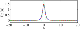
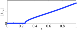
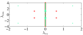
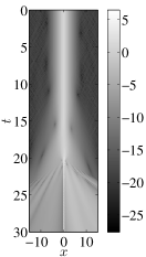
Figure 1: Top left and middle panels show, respectively, the profiles of Re$(u)$ and Im$(u)$ for $\epsilon=0$ (solid), $\epsilon=0.2$ (dashed), $\epsilon=0.5$ (dashed-dotted), and $\epsilon=1$ (dotted). The bottom left panel shows the maximal real part of the linearization eigenvalues $\lambda$ as a function of $\epsilon$, showcasing the instability beyond $\epsilon=0.257$. The bottom middle panel shows the spectral plane of the imaginary vs. the real part of $\lambda$ for $\epsilon=0$ (dots), $\epsilon=0.2$ (squares), $\epsilon=0.5$ (circles), and $\epsilon=1.0$ (crosses). Right panel: Space-time contour plot of the evolution of the density $|u|^{2}$ (in logarithmic scale) of an unstable soliton for $\epsilon=0.4$.

We start with the case $k=1$ and $\sigma=-1$, for which the density $\rho(x)$ has the form of a bright soliton and the respective potential $W(x)$ is ${\cal PT}$-symmetric, as obtained in Eq. (7). In the top left and middle panels of Fig. 1, we show the real and imaginary parts of the solution; it is observed that the former remains symmetric, while its imaginary part develops an anti-symmetric profile of increasing magnitude as $\epsilon$ increases. On the other hand, see bottom left and middle panels of Fig. 1, it is interesting to observe the corresponding stability characteristics of the solution. Rather unusually (especially for bright solitons in single-component NLS models), the spectrum features an oscillatory instability beyond the critical value of $\epsilon=0.257$. The relevant instability eigenvalue quartet features both a real and an imaginary part, indicating the concurrent presence of growth (with a rate associated with the real part) and oscillation (with a frequency associated with the imaginary part). While such instabilities have been identified previously, e.g., for bound states of two or more solitons [17], we are not aware of cases in Hamiltonian models, where the breaking of translational invariance for a single soliton due to the presence of an external potential leads to an oscillatory instability. In the Hamiltonian case, this can be explained based on the positive Krein signature (i.e., concavity of the energy surface) along the eigendirection of the mode associated with translation [18]. Interestingly, the notion of energy associated with a given mode or Krein signature has not been extended to the presence of gain and loss. Nevertheless, it can be clearly seen that the eigenvalues still arise in pairs or quartets as in the Hamiltonian case. This advocates both the relevance and importance of developing an extension of the Krein signature for such ${\cal PT}$-symmetric settings.

We now turn to direct numerical simulations exploring the dynamics of such bright soliton solutions. The right panel in Fig. 1 corresponds to the unstable case of $\epsilon=0.4$. The scale shown in the space-time contour plot is logarithmic, so that the excessive growth associated with the exponential instability does not obscure the development of the oscillatory instability.

We note that we observed results similar to the ones presented above for the case $k=2$ and $\sigma=-1$ (focusing nonlinearity); for instance, when using the potential $W(x)=-4\sqrt{2}\epsilon\,\,{\rm sech}(\sqrt{2}x)\tanh(\sqrt{2}x)$, the only difference we found lies in the location of the critical point (occurring at $\epsilon=0.247$).

3.2 The case $k=2$ and $\sigma=+1$ (defocusing nonlinearity)

We now consider the case $k=2$ and $\sigma=+1$ (defocusing nonlinearity), which leads to the ${\cal PT}$-symmetric potential in Eq. (12). The existence and stability results for the relevant dark soliton solutions are illustrated in Fig. 2. Here, similarly to the results of Ref. [20], in the top panels it is observed that while the real part of the dark soliton remains anti-symmetric, its imaginary part develops a symmetric, sech-shaped profile, on the background of a homogeneous, non-vanishing pedestal. As concerns their stability, these states are unstable due to the emergence of real eigenvalue pairs, for all values of $\epsilon$; this family of solutions can only be followed until $\epsilon=0.544$ (see below). The bottom left panel of Fig. 2 shows that the maximum of the (absolute) real part of the eigenvalues, is increasing with increasing $\epsilon$. Note that the imaginary part of the unstable eigenvalues was found to be zero for all $\epsilon$. In particular, it is found that the corresponding spectra (not shown here) exhibit increasingly more unstable eigenvalues, by increasing $\epsilon$. The latter suggests that, not only the soliton but also the background becomes unstable. An example of the instability dynamics is shown in the bottom right panel of the same figure, for $\epsilon=0.4$. It is observed that the soliton remains quiescent for some time, but then it is spontaneously ejected to the “gain” side of the imaginary potential (for $x>0$) and starts moving with a finite velocity away from the origin. This behavior can be qualitatively explained by the fact that the soliton feels an effective potential [20].

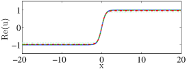
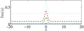
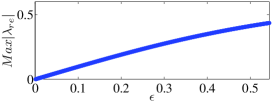
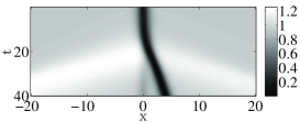
Figure 2: The top left (right) panel shows the real (imaginary) part of the dark soliton solutions for $\epsilon=0.01$ (solid), $\epsilon=0.2$ (dashed), $\epsilon=0.4$ (dashed-dotted), and $\epsilon=0.54$ (dotted). The bottom left panel shows the most unstable real eigenvalue as a function of $\epsilon$. The bottom right panel shows a space-time contour plot of the evolution for $\epsilon=0.4$.

Additionally, as observed in the bottom right panel of Fig. 2, at $x=0$ there exists a shallow, stationary localized dip for all times, suggesting the existence of still another stationary, and in this case stable, state. In fact, it is possible to find this branch, for the same potential $W(x)$ [cf. Eq. (12)], by performing numerical continuation in $\epsilon$, starting from the plane wave solution of the NLS Eq. (1) —alternatively, this branch can be found in an approximate analytical form, using the methodology of Ref. [20]. This branch corresponds to the ground state of the system, and its real and imaginary parts are respectively shown in the left and middle panels of Fig. 3. Note that the real part of the solutions has a sech-shaped bump localized at the origin (similar to the imaginary part of the dark soliton), while its imaginary part is tanh-shaped (similar to the real part of the dark soliton). As is expected, the ground state branch coexists with the excited sate (the soliton), up to a certain critical value of $\epsilon$; at this value, the branches collide and disappear via a saddle-center bifurcation, in a way similar to the nonlinear ${\cal PT}$-phase transition [20]. This is illustrated in the right panel of Fig. 3, where the norms $\|u\|_{L^{2}}$ of the above mentioned branches are shown as functions of $\epsilon$ (the critical value of $\epsilon$ is found to be $\epsilon=0.544$).

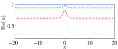
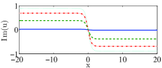
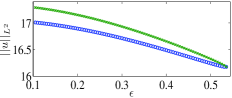
Figure 3: The left (middle) panel shows the real (imaginary) part of another branch of solutions for $\epsilon=0$ (solid), $\epsilon=0.2$ (dashed), $\epsilon=0.4$ (dashed-dotted), and $\epsilon=0.54$ (dotted). The right panel shows the bifurcation diagram of the $L^{2}$ norm of the branch stemming from the homogeneous states (green crosses) and the one of the dark solitons (blue circles); the saddle-center bifurcation occurs at $\epsilon=0.544$.

3.3 The case of a modified ${\cal PT}$-symmetric potential

In the previous case of $k=2$, and for $W(x)$ given by Eq. (12), we found that soliton solutions gradually became highly unstable due to the fact that, not only the solitons, but also their backgrounds became unstable. For this reason, we investigate a modified version of $W(x)$, namely the ${\cal PT}$-symmetric potential $W(x)=2\epsilon\,\,{\rm sech}^{2}(x)\tanh(x)$. Although exact analytical dark soliton solutions are not available in this setting, one can obtain soliton solutions numerically. In fact, we have found such a soliton branch, with profiles similar to those shown in the top panels of Fig. 2; we also found that this branch disappears at $\epsilon=0.469$. Accordingly, a stability analysis for this soliton branch shows (see left panel of Fig. 4) that the maximum unstable (real) eigenvalue departs from the origin, performs a maximal excursion and subsequently return to the origin at $\epsilon=0.469$, in a way reminiscent of a bifurcation. An additional important difference of these soliton states with the ones corresponding to $W(x)$ in Eq. (12) is that, now, the instability is caused by a single real eigenvalue pair —cf. middle panel of Fig. 4. This eigenvalue pair, is associated with the motion of the dark soliton [20]; the absence of other unstable eigenvalues suggests that, while the dark soliton is unstable, the background is not —unlike the previous case of $W(x)$ in Eq. (12), where the presence of many unstable modes indicated the instability of the background.

An example of the dynamics of an unstable soliton evolving in the presence of the modified potential $W(x)$, is shown in the right panel of Fig. 4. Evidently, the instability renders the soliton mobile, in a similar way as in the bottom right panel of Fig. 2. Additionally, as in the case of $W(x)$ given by Eq. (12), there exists a persistent localized structure at $x=0$, adjacent to the soliton. As before, we can associate this structure with the existence of another branch of solutions, which can be obtained by a continuation, starting from a plane wave solution at $\epsilon=0$. We have numerically obtained this ground state branch, and it was found to have a similar profile as the one shown in the left and middle panels of Fig. 3. We have also confirmed that this branch collides with the soliton branch at $\epsilon=0.469$, where they disappear through a saddle-center bifurcation, similar to what is shown in the right panel of Fig. 3. It is important to note that, contrary to the previous case of $W(x)$ given by Eq. (12), this branch is found to be stable throughout its existence regime; furthermore, we have confirmed that the localized structure at $x=0$, shown in the right panel of Fig. 4, is identical to the exact solution profile of the ground state branch.

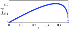
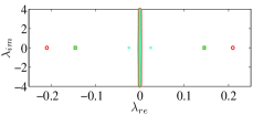
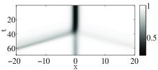
Figure 4: Left panel: the most unstable real eigenvalue, performing a maximal excursion over $\epsilon$, before returning to collide with the origin at $\epsilon=0.469$. Middle panel: spectral plane for $\epsilon=0$ (dots), $0.2$ (squares), $0.4$ (circles), $0.469$ (crosses). Right panel: space-time contour plot showing the evolution of the soliton density for $\epsilon=0.4$.

4 Conclusions and Future Challenges

Concluding, we have studied a class of ${\cal PT}$-symmetric NLS models, in which their hydrodynamic form can be reduced to a Duffing or a generalized Duffing equation. From this type of reduction, we were able to extract a number of cases bearing exact analytical soliton solutions. The stability and dynamics of these solutions were studied numerically, and a number of intriguing features were found. In particular, we presented cases where bright solitons in a single-component, ${\cal PT}$-symmetric NLS equation are subject to an oscillatory instability, a trait absent in the Hamiltonian installments of the model. This underscored the need for generalizing the notion of Krein signature in such systems. On the other hand, for defocusing nonlinearities, a saddle-center bifurcation reminiscent of the ${\cal PT}$-phase transition was found between the ground state (plane wave in the Hamiltonian limit) and the first excited state (a dark soliton in the Hamiltonian limit). Connections of all these features to earlier works were also given. We also note that we have studied cnoidal wave solutions (results not shown), which were found to be dynamically unstable.

There are many interesting future directions associated with this work. In the 1D setting, it is important to understand topological notions, such as the Krein signature, and other stability characteristics of solutions of ${\cal PT}$-symmetric systems, as well as their connections to the Hamiltonian analogs. On the other hand, admittedly even for the existence problem, there are some intriguing questions (such as the difference in the bifurcation structure between the cases of focusing and defocusing nonlinearities). Furthermore, while numerous studies have, by now, developed in the 1D realm, two- (and higher-) dimensional explorations are presently far more limited. Hence, this is also a direction of considerable interest for future studies.

References

- [1] C.M. Bender and S. Boettcher, Phys. Rev. Lett. 80, 5243 (1998).
- [2] C.M. Bender, Rep. Prog. Phys. 70, 947 (2007).
- [3] A. Ruschhaupt, F. Delgado, and J.G. Muga, J. Phys. A: Math. Gen. 38, L171 (2005).
- [4] Z.H. Musslimani et al., Phys. Rev. Lett. 100, 030402 (2008).
- [5] K.G. Makris et al., Phys. Rev. A 81, 063807 (2010).
- [6] H. Ramezani et al., Phys. Rev. A 82, 043803 (2010).
- [7] M. Kulishov and B. Kress, Opt. Express 20, 29319 (2012).
- [8] C.E. Rüter et al., Nat. Phys. 6, 192 (2010).
- [9] A. Guo et al., Phys. Rev. Lett. 103, 093902 (2009).
- [10] J. Schindler et al., Phys. Rev. A 84, 040101 (2011).
- [11] J. Schindler et al., J. Phys. A: Math. Theor. 45, 444029 (2012).
- [12] B. Peng et al., arXiv:1308.4564v1.
- [13] Y. He and D. Mihalache, Rom. Rep. Phys. 64, 1243 (2012).
- [14] Z. Ahmed, Phys. Lett. A 282, 343 (2001).
- [15] B. Midya and R. Roychoudhury, Phys. Rev. A 87, 045803 (2013).
- [16] M. Salerno, arXiv:1306.3643v1.
- [17] P.G. Kevrekidis et al., New J. Phys. 5, 64 (2003).
- [18] T. Kapitula, P.G. Kevrekidis, B. Sandstede, Phys. D 195, 263 (2004).
- [19] R. S. MacKay, in: Hamiltonian Dynamical Systems, Hilger, Bristol (1987), p. 137.
- [20] V. Achilleos et al., Phys. Rev. A 86, 013808 (2012).