Stochastic Turing patterns: analysis of compartment-based approaches

Abstract

Turing patterns can be observed in reaction-diffusion systems where chemical species have different diffusion constants. In recent years, several studies investigated the effects of noise on Turing patterns and showed that the parameter regimes, for which stochastic Turing patterns are observed, can be larger than the parameter regimes predicted by deterministic models, which are written in terms of partial differential equations for species concentrations. A common stochastic reaction-diffusion approach is written in terms of compartment-based (lattice-based) models, where the domain of interest is divided into artificial compartments and the number of molecules in each compartment is simulated. In this paper, the dependence of stochastic Turing patterns on the compartment size is investigated. It has previously been shown (for relatively simpler systems) that a modeller should not choose compartment sizes which are too small or too large, and that the optimal compartment size depends on the diffusion constant. Taking these results into account, we propose and study a compartment-based model of Turing patterns where each chemical species is described using a different set of compartments. It is shown that the parameter regions where spatial patterns form are different from the regions obtained by classical deterministic PDE-based models, but they are also different from the results obtained for the stochastic reaction-diffusion models which use a single set of compartments for all chemical species. In particular, it is argued that some previously reported results on the effect of noise on Turing patterns in biological systems need to be reinterpreted.

1 Introduction

In his pioneering work, Alan Turing Turing:1952:CBM showed that stable spatial patterns can develop in reaction-diffusion systems which include chemical species (morphogens) with different diffusion constants. Considering a system of two chemical species with concentrations $u(x,t)$ and $v(x,t)$ in one-dimensional interval $x\in[0,L]$, the underlying deterministic model of Turing patterns can be written as a system of two reaction-diffusion partial differential equations (PDEs)

$$\frac{\partial u}{\partial t} = D_{u}\frac{\partial^{2}u}{\partial x^{2}}+f_{1}(u,v),$$ (1.1)

$$\frac{\partial v}{\partial t} = D_{v}\frac{\partial^{2}v}{\partial x^{2}}+f_{2}(u,v),$$ (1.2)

where $D_{u}$ and $D_{v}$ are diffusion constants of morphogens $u$ and $v$, respectively, and $f_{1}(u,v)$ and $f_{2}(u,v)$ describe chemical reactions. Then the standard analysis proceeds as follows Murray:2002:MB ; Satnoianu:2000:TIG : a homogeneous steady state $u(x,t)\equiv u_{s}$, $v(x,t)\equiv v_{s}$ is found by solving $f_{1}(u_{s},v_{s})=0$ and $f_{2}(u_{s},v_{s})=0$. It is shown that the homogenous steady state is stable when $D_{u}=D_{v}$, and conditions on $f_{1}$, $f_{2}$, $D_{u}$ and $D_{v}$ are obtained which guarantee that the homogeneous steady state will become unstable for $D_{u}\neq D_{v}$. Then Turing patterns are observed at the steady state.

The above argument was extensively analysed in the mathematical biology literature and conditions for Turing patterns have been determined Murray:2002:MB ; Satnoianu:2000:TIG . Experimental studies with chemical systems (chlorite-iodide-malonic acid reaction) demonstrated Turing type patterns Kepper:1991:TCP ; Quyang:1991:TUS . There has also been experimental evidence that a simple Turing patterning mechanism can appear in developmental biology, for example, in the regulation of hair follicle patterning in developing murine skin Sick:2006:WDD . One of the criticism of Turing patters is their lack of robustness Maini:2012:TMB . The PDE system (1.1)–(1.2) can have several stable non-homogeneous solutions which the system can achieve with relatively small perturbations to the initial condition. Considering PDEs in a suitably growing domain, one can obtain an additional constraint on the system which restricts the set of accessible patterns, increasing the robustness of pattern generation with respect to the initial conditions Crampin:1999:RDG ; Barrass:2006:MTM . However, to assess the sensitivity of patterns with respect to fluctuations, stochastic models have to be considered Maini:2012:TMB ; Black:2012:SFE .

One of the most common approaches to stochastic reaction-diffusion modelling is formulated in the compartment-based (lattice-based) framework Erban:2007:PGS . In the one-dimensional setting, the compartment-based analogue of the PDE model (1.1)–(1.2) can be formulated as follows: The computational domain $[0,L]$ is divided into $K$ compartments of length $h=L/K$. We denote the number of molecules of chemical species $U$ (resp. $V$) in the $i$-th compartment $((i-1)h,ih)$ by $U_{i}$ (resp. $V_{i}$), $i=1,2,\dots,K$. Then the diffusion of $U$ and $V$ is described by the following chains of “chemical reactions” Erban:2007:PGS :

$$U_{1}\;\mathop{\stackrel{{\scriptstyle\displaystyle\longrightarrow}}{{\longleftarrow}}}^{d_{u}}_{d_{u}}\;U_{2}\;\mathop{\stackrel{{\scriptstyle\displaystyle\longrightarrow}}{{\longleftarrow}}}^{d_{u}}_{d_{u}}\;U_{3}\;\mathop{\stackrel{{\scriptstyle\displaystyle\longrightarrow}}{{\longleftarrow}}}^{d_{u}}_{d_{u}}\;\dots\;\mathop{\stackrel{{\scriptstyle\displaystyle\longrightarrow}}{{\longleftarrow}}}^{d_{u}}_{d_{u}}\;U_{K},$$ (1.3)

$$V_{1}\;\mathop{\stackrel{{\scriptstyle\displaystyle\longrightarrow}}{{\longleftarrow}}}^{d_{v}}_{d_{v}}\;V_{2}\;\mathop{\stackrel{{\scriptstyle\displaystyle\longrightarrow}}{{\longleftarrow}}}^{d_{v}}_{d_{v}}\;V_{3}\;\mathop{\stackrel{{\scriptstyle\displaystyle\longrightarrow}}{{\longleftarrow}}}^{d_{v}}_{d_{v}}\;\dots\;\mathop{\stackrel{{\scriptstyle\displaystyle\longrightarrow}}{{\longleftarrow}}}^{d_{v}}_{d_{v}}\;V_{K}$$ (1.4)

where

$$d_{u}=\frac{D_{u}}{h^{2}}\qquad\mbox{and}\qquad d_{v}=\frac{D_{v}}{h^{2}}.$$ (1.5)

Reactions are localized to each compartment. For example, considering the commonly studied Schnakenberg reaction system Schnakenberg:1979:SCR , chemical reactions in the $i$-th compartment are described by Qiao:2006:SDS :

$${\mbox{ \raise 2.42131pt\hbox{$\emptyset$}}}\;\mathop{\stackrel{{\scriptstyle\displaystyle\longrightarrow}}{{\longleftarrow}}}^{k_{1}}_{k_{2}}\;{\mbox{\raise 2.42131pt\hbox{$U_{i}$,}}}\qquad\qquad\mbox{ \raise 2.84526pt\hbox{$\emptyset\;\displaystyle\mathop{\displaystyle\longrightarrow}^{k_{3}}\;V_{i}$,}}\qquad\qquad\mbox{ \raise 2.84526pt\hbox{$2U_{i}+V_{i}\;\displaystyle\mathop{\displaystyle\longrightarrow}^{k_{4}}\;3U_{i}$.}}$$ (1.6)

The above formulation (1.3), (1.4) and (1.6) describes the stochastic reaction-diffusion model as a system of ($8K-4$) chemical reactions: we have ($K-1$) diffusive jumps of $U$ molecules to the left (resp. right), ($K-1$) diffusive jumps of $V$ molecules to the left (resp. right), and $4K$ reactions (1.6). This system can be simulated using the Gillespie algorithm Gillespie:1977:ESS , or its equivalent formulations Cao:2004:EFS ; Gibson:2000:EES . In Figure 1, we present an illustrative simulation of the reaction-diffusion system (1.3), (1.4) and (1.6). We clearly see that Turing patterns can be observed for the chosen set of dimensionless parameters:

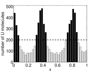
     (a)   (b)

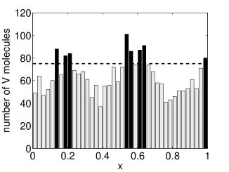
Figure 1: Turing patterns for the stochastic reaction-diffusion system $(\ref{diffGillU})$, $(\ref{diffGillV})$ and $(\ref{schnak})$. (a) Numbers of molecules of chemical species $U$ in each compartment at time $18$; (b) the same plot for chemical species $V$. The initial condition was the homogeneous steady state $U_{st}=200$ and $V_{st}=75$ for the parameters given in the text. The values of $U_{st}$ and $V_{st}$ are denoted by dashed lines. Adapted from Erban:2007:PGS with permission.

$k_{1}=4\times 10^{3}$, $k_{2}=2$, $k_{3}=1.2\times 10^{3}$, $k_{4}=6.25\times 10^{-8}$, $D_{u}=10^{-3}$ and $D_{v}=10^{-1}$. Compartment values above (resp. below) the homogeneous steady state values $U_{st}=200$ and $V_{st}=75$ are coloured black (resp. light gray) to visualize stochastic Turing patterns. Let us note that the rate constants $k_{1}$ and $k_{3}$ are production rates per unit of area. The stochastic model uses the production rates per one compartment which are given as $k_{1}h$ and $k_{3}h$, respectively. More details of this stochastic simulation are given in Section 2 where we introduce the corresponding propensity functions (2.4)–(2.5).

The compartment-based approach has been used for both theoretical analysis and computational modelling Scott:2011:AIN ; Hattne:2005:SRD . The regions where stochastic Turing patterns can be expected were calculated using the linear noise analysis Biancalani:2010:STP ; McKane:2013:SPF ; Butler:2011:FTP . These studies were also generalized to growing domains Woolley:2011:PSM ; Woolley:2011:SRD , to stochastic reaction-diffusion models with delays Woolley:2012:EIS , to non-local trimolecular reactions Biancalani:2011:SWB and to stochastic Turing patterns on a network Asslani:2012:STP . Compartment-based software packages were developed Hattne:2005:SRD and applied to modelling biological systems Fange:2006:NMP . Computational approaches were also generalized to non-regular compartments (lattices) and complex geometries Engblom:2009:SSR ; Isaacson:2006:IDC . Stochastic simulations of Turing patterns Twomey:2007:SMR ; Fu:2008:SST ; Hori:2012:NSP and excitable media Vigelius:2012:SSP were also presented in the literature. However, these theoretical and computational studies use the same discretization for each chemical species. In this paper, we will demonstrate that, in the case of Turing patterns, this simplifying assumption can undesirably bias the obtained theoretical and computational results.

One of the assumption of the compartment-based modelling is that compartments are small enough so that they can be assumed well-mixed. In particular, the relative size of diffusion and reaction constants determine the appropriate size of the compartment Erban:2009:SMR ; Isaacson:2009:RME ; Hellander:2012:RME . It can be shown that there exists a limitation on the compartment size from below whenever the reaction-diffusion system includes a bimolecular reaction Erban:2009:SMR ; Isaacson:2009:RME ; Hellander:2012:RME . There are also bounds on the compartment size from above Kang:2012:NMC ; Hu:2013:SAR , again the diffusion constant plays an important role in these estimates. In the case of Turing patterns, we have chemical species with different diffusion constants. For example, in the illustrative simulation in Figure 1, we have $D_{v}/D_{u}=100$, i.e. the diffusion constant of $V$ is 100-times larger than the diffusion constant of $U$. However, we used the same discretization for both $U$ and $V$ which is schematically denoted in Figure 2(a).

  (a)            (b)

Figure 2: (a) Schematic of the uniform discretization. (b) Schematic of different meshes used for $U$ and $V$ where $\gamma$ defined by $(\ref{definitionhuhv})$ is equal to 5.

If we take into account that $V$ diffuses much faster, then one could also consider the discretization in Figure 2(b) where one compartment in the $V$ variable corresponds to several compartments in the $U$ variable. In this paper, we will study differences between discretizations in Figure 2(a) and Figure 2(b). We will show that these discretizations lead to different parameter regimes for stochastic Turing patterns.

The paper is organized as follows. In Section 2 we introduce and analyse a simple test problem which will be used to illustrate our results. It will be based on the above model (1.3), (1.4) and (1.6). In Section 3 we analyse both types of discretizations, considering a simple two-compartment discretization in $U$. Illustrative numerical results are presented in Section 4. We conclude this paper with the discussion of our results in Section 5.

2 Deterministic and stochastic models of an illustrative reaction-diffusion system

We will consider a simple one-dimensional Schnakenberg model (1.6) where the reaction rate constants are given by Qiao:2006:SDS

$$k_{1}=\omega,\qquad k_{2}=2,\qquad k_{3}=3\omega,\qquad k_{4}=\frac{1}{\omega^{2}}$$ (2.1)

and $\omega$ is a scale factor. We used $\omega=4\times 10^{3}$ in the illustrative simulation in Figure 1. When there is no diffusion involved, the dynamics of this system can be represented as the system of reaction rate ordinary differential equations (ODEs)

$$\frac{\mbox{d}u}{\mbox{d}t} = k_{1}-k_{2}u+k_{4}u^{2}v,$$

$$\frac{\mbox{d}v}{\mbox{d}t} = k_{3}-k_{4}u^{2}v,$$

which has a unique stable steady state at $u_{s}=2\omega$ and $v_{s}=3\omega/4$. When we consider diffusion, the reaction-diffusion PDEs (1.1)–(1.2) are given by

$$\frac{\partial u}{\partial t} = D_{u}\frac{\partial^{2}u}{\partial x^{2}}+k_{1}-k_{2}u+k_{4}u^{2}v,$$ (2.2)

$$\frac{\partial v}{\partial t} = D_{v}\frac{\partial^{2}v}{\partial x^{2}}+k_{3}-k_{4}u^{2}v.$$ (2.3)

We are implicitly assuming homogeneous Neumann boundary conditions (zero-flux) in the whole paper, but both the PDE model (2.2)–(2.3) and its stochastic counterparts could also be generalized to different types of boundary conditions Erban:2007:RBC . Using standard analysis of Turing instabilities Qiao:2006:SDS ; Murray:2002:MB , one can show that the Turing patterns are obtained for $D_{v}>39.6D_{u}$ for the parameter values (2.1). This condition is independent of $\omega.$ The illustrative simulation in Figure 1 was computed for $D_{v}/D_{u}=100$, i.e. the condition for (deterministic, mean-field) Turing patterns was satisfied.

When we are concerned with the stochastic effects, the reaction-diffusion system can be simulated by the Gillespie stochastic simulation algorithm with the one-dimensional computational domain $[0,L]$ discretized. Considering uniform discretization in Figure 2(a), the stochastic model is given as a set of “chemical reactions” (1.3), (1.4) and (1.6). Denoting the compartment length by $h$, we have the following propensity functions in the $i$-th compartment Gillespie:1977:ESS ; Qiao:2006:SDS :

$$\alpha_{1}=k_{1}h,\quad\alpha_{2}=k_{2}U_{i},\quad\alpha_{3}=k_{3}h,\quad\alpha_{4}=\frac{k_{4}}{h^{2}}U_{i}(U_{i}-1)V_{i},$$ (2.4)

$$\alpha_{5}=\alpha_{6}=d_{u}U_{i},\qquad\qquad\alpha_{7}=\alpha_{8}=d_{v}V_{i},$$ (2.5)

where $d_{u}$ and $d_{v}$ are given by (1.5). The first four propensities (2.4) are for the four chemical reactions in (1.6). The propensities (2.5) are for the diffusive jumps (left and right) for $U$ (indices 5 and 6) and $V$ (indices 7 and 8) which correspond to (1.3) and (1.4), respectively. In the illustrative simulation in Figure 1, we divided interval $[0,1]$ into $K=40$ compartments, i.e. $h=1/40=0.025$. In particular, the production rate of $U$ molecules in one compartment was equal to $\alpha_{1}=k_{1}h=\omega h=100$. The homogeneous steady state in compartments corresponded to values $U_{st}=u_{s}h=2\omega h=200$ and $V_{st}=v_{s}h=3h\omega/4=75.$

2.1 Formulation of the generalized comparment-based model

The compartmentalization in Figure 2(b) generalizes (1.3) and (1.4) to the case where different discretizations are used for $U$ and $V$. We will denote by $K_{u}$ (resp. $K_{v}$) the number of compartments in the $U$ (resp. $V$) variable. We define the compartment lengths by

$$h_{u}=\frac{L}{K_{u}},\qquad h_{v}=\frac{L}{K_{v}},\qquad\mbox{and}\qquad\gamma=\frac{K_{u}}{K_{v}}=\frac{h_{v}}{h_{u}},$$ (2.6)

where $\gamma$ is the ratio of compartment sizes in the $V$ and $U$ variable. In what follows, we will consider that $\gamma$ is an integer. For example, a schematic diagram in Figure 2(b) used $\gamma=5$. Then the diffusion model is formulated as follows

$$U_{1}\;\mathop{\stackrel{{\scriptstyle\displaystyle\longrightarrow}}{{\longleftarrow}}}^{d_{u}}_{d_{u}}\;U_{2}\;\mathop{\stackrel{{\scriptstyle\displaystyle\longrightarrow}}{{\longleftarrow}}}^{d_{u}}_{d_{u}}\;U_{3}\;\mathop{\stackrel{{\scriptstyle\displaystyle\longrightarrow}}{{\longleftarrow}}}^{d_{u}}_{d_{u}}\;\dots\;\mathop{\stackrel{{\scriptstyle\displaystyle\longrightarrow}}{{\longleftarrow}}}^{d_{u}}_{d_{u}}\;U_{K_{u}},$$ (2.7)

$$V_{1}\;\mathop{\stackrel{{\scriptstyle\displaystyle\longrightarrow}}{{\longleftarrow}}}^{d_{v}}_{d_{v}}\;V_{2}\;\mathop{\stackrel{{\scriptstyle\displaystyle\longrightarrow}}{{\longleftarrow}}}^{d_{v}}_{d_{v}}\;V_{3}\;\mathop{\stackrel{{\scriptstyle\displaystyle\longrightarrow}}{{\longleftarrow}}}^{d_{v}}_{d_{v}}\;\dots\;\mathop{\stackrel{{\scriptstyle\displaystyle\longrightarrow}}{{\longleftarrow}}}^{d_{v}}_{d_{v}}\;V_{K_{v}},$$ (2.8)

where

$$d_{u}=\frac{D_{u}}{h_{u}^{2}},\qquad\qquad d_{v}=\frac{D_{v}}{h_{v}^{2}}=\frac{D_{v}}{D_{u}\gamma^{2}}\,d_{u}.$$ (2.9)

In the standard comparment-based model (1.3) and (1.4), we have $\gamma=1$. One option to choose $\gamma$ in the generalized model (2.7) and (2.8) is to ensure that $d_{u}=d_{v}$ which implies

$$\gamma=\sqrt{\frac{D_{v}}{D_{u}}}.$$ (2.10)

Then the jump rates $d_{u}$ and $d_{v}$ from the corresponding compartments are equal for molecules of $U$ and $V$. However, we will not restrict to the case (2.10) and consider general choices of $\gamma$ in this paper. The generalization of the first three propensities in (2.4) is straightforward. Propensities $\alpha_{1}$ and $\alpha_{2}$ in (2.4) correspond to chemical species $U$ and we have the following propensities in the $i$-th compartment, $i=1,2,\dots,K_{u}$: $\alpha_{1}=k_{1}h_{u}$ and $\alpha_{2}=k_{2}U_{i}$. The propensity $\alpha_{3}$ in (2.4) is considered in the $j$-th compartment corresponding to the $V$ species, i.e. in the compartment $\big{(}(j-1)h_{v},jh_{v}\big{)}$. It is given as $\alpha_{3}=k_{3}h_{v}$. To generalize $\alpha_{4}$, we have to consider the occurrences of the trimolecular reaction

$$2U+V\;\displaystyle\mathop{\displaystyle\longrightarrow}^{k_{4}}\;3U$$

in every small compartment in discretization of the $U$ variable. In the $i$-th compartment, the propensity function $\alpha_{4}$ is:

$$\alpha_{4}=\frac{k_{4}}{h_{u}^{2}}U_{i}(U_{i}-1)\frac{V_{j}}{\gamma},$$ (2.11)

where $V_{j}$ corresponds to the $j$-th compartment in the $V$ variable to which the $i$-th compartment belongs, i.e.

$$\big{(}(i-1)h_{u},ih_{u}\big{)}\subset\big{(}(j-1)h_{v},jh_{v}\big{)}.$$

The main idea of the compartment-based model is that the molecules of $V$ are considered to be well-mixed in the compartments of the size $h_{v}$. Thus the propensity function (2.11) correctly generalizes the propensity of trimolecular reaction $\alpha_{4}$ in the smaller compartment of length $h_{u}$.

In Figure 3, we present an illustrative simulation of the generalized compartment-based model (2.7)–(2.11). We use the same parameters as in Figure 1 to enable direct comparisons, i.e. $k_{1}$, $k_{2}$, $k_{3}$, $k_{4}$ are given by (2.1) where the scale factor $\omega=4\times 10^{3}$. We use (2.10) to select the value of $\gamma$. Since $D_{u}=10^{-3}$ and $D_{v}=10^{-1}$, the formula (2.10) implies $\gamma=10$. We use the same number of compartments for $U$ variable as in Figure 1: $K_{u}=40$. Using $\gamma=10$, we obtain that $V$ is discretized into $K_{v}=4$ compartments. In Figure 3, we see that the Turing pattern can still be clearly observed. As in Figure 1,

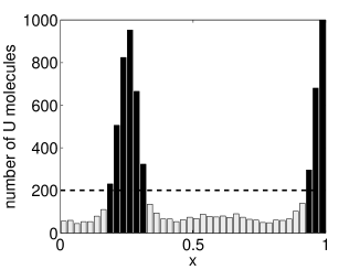
     (a)   (b)

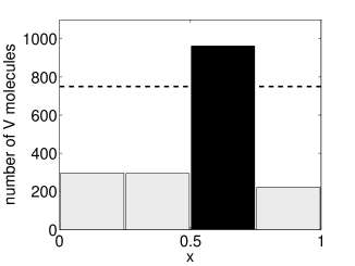
Figure 3: Turing patterns computed by the generalized compartment-based model $(\ref{diffGillUm})$–$(\ref{generalizationofalpha4})$. (a) Numbers of molecules of chemical species $U$ in each compartment at time $18$; (b) the same plot for chemical species $V$. The initial condition was the homogeneous steady state $U_{st}=200$ and $V_{st}=750$ for the parameters given in the text. The values of $U_{st}$ and $V_{st}$ are denoted by dashed lines.

compartment values above (resp. below) the homogeneous steady state values $U_{st}=200$ and $V_{st}=75\gamma=750$ are coloured black (resp. light gray) to visualize stochastic Turing patterns.

Since the compartments in $V$ variable are 10-times larger in Figure 3(b) then in Figure 1(b), it is not suprising that the numbers of molecules of $V$ (per compartment) increased by the factor of 10. However, we can also notice that the numbers of molecules of $U$ per compartment quantitatively differ in Figure 1(a) and Figure 3(a) (black peaks are twice taller). An open question is to quantify these differences. In this paper, we will study even more fundamental issue: we will see that we can find parameter regimes where the generalized compartment-based model exhibits Turing patterns, while the original discretization does not.

The generalized compartment-based model (2.7) and (2.8) can be used to construct computational approaches to speed-up simulations of the standard compartment-based model, because it does not simulate all diffusion events for chemical species with large diffusion constants LiCao2012 ; LiCao2013 . For example, the illustrative simulation in Figure 3 simulates ten times less compartments for $V$ and is less computationaly intensive than the original simulation in Figure 1. However, in this work, we are interested in a different question than discussing different numerical errors with different discretization strategies. We will investigate the Turing pattern formation under different discretizations. We will argue that the classical compartment-based approach is not the best starting point to analyse noise in systems which have chemical species with different diffusion constants. This conclusion can be already demonstrated if we consider a simple two-compartment model as we will see in the next section.

3 Analysis of compartment-based models for $K_{u}=2$

We will consider that the domain $[0,L]$ is divided into two compartments in the $U$ variable, i.e. $K_{u}=2.$ Then we have two possible options for the discretization of the quickly diffusing chemical species $V$:

(i) $\gamma=1$ which corresponds to the classical compartment-based model where $K_{v}=2$;

(ii) $\gamma=2$ which corresponds to the generalized compartment-based model where $K_{v}=1$.

We will start with the latter case which includes three variables $U_{1}$, $U_{2}$ and $V_{1}$ and is easier to analyse. In Section 3.2 we compare our results with the classical compartment-based approach.

3.1 Generalized compartment-based model: $K_{u}=2$ and $K_{v}=1$

We consider the case where the whole interval $[0,\ L]$ is divided into two compartments for $U$ and one compartment for $V$. The discretization is illustrated in Figure 4(a).

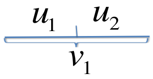
  (a)            (b)

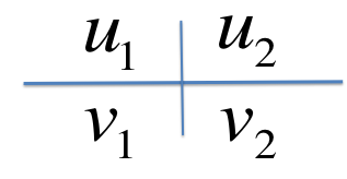
Figure 4: (a) Generalized compartment-based model for $K_{u}=2$ and $K_{v}=1$: The interval is divided into two compartments for $U$ and remains as one compartment for $V$. (b) Classical compartment-based model: The interval is divided into two compartments for both $U$ and $V$.

We will denote by $u_{1}$, $u_{2}$ and $v_{1}$ the average numbers of molecules of $U_{1}$, $U_{2}$ and $V_{1}$ as predicted by the corresponding mean-field model. They satisfy the following system of three ODEs Erban:2007:PGS

$$\frac{\mbox{d}u_{1}}{\mbox{d}t} = d_{u}(u_{2}-u_{1})+k_{1}h_{u}-k_{2}u_{1}+\frac{k_{4}}{h_{u}h_{v}}u_{1}^{2}v_{1},$$ (3.1)

$$\frac{\mbox{d}u_{2}}{\mbox{d}t} = d_{u}(u_{1}-u_{2})+k_{1}h_{u}-k_{2}u_{2}+\frac{k_{4}}{h_{u}h_{v}}u_{2}^{2}v_{1},$$ (3.2)

$$\frac{\mbox{d}v_{1}}{\mbox{d}t} = k_{3}h_{v}-\frac{k_{4}}{h_{u}h_{v}}\left(u_{1}^{2}+u_{2}^{2}\right)v_{1}.$$ (3.3)

We will study the stability of its steady states. In order to find the steady state, we let the left hand side terms be zero. The corresponding algebraic equations can be written in the following form:

$$d_{u}(u_{2}-u_{1})+\frac{k_{1}L}{2}-k_{2}u_{1}+\frac{2k_{4}}{L^{2}}\,u_{1}^{2}v_{1} = 0,$$ (3.4)

$$d_{u}(u_{1}-u_{2})+\frac{k_{1}L}{2}-k_{2}u_{2}+\frac{2k_{4}}{L^{2}}\,u_{2}^{2}v_{1} = 0,$$ (3.5)

$$k_{3}L-\frac{2k_{4}}{L^{2}}\,(u_{1}^{2}+u_{2}^{2})v_{1} = 0,$$ (3.6)

where we used $h_{u}=L/K_{u}=L/2$ and $h_{v}=L/K_{v}=L.$ Adding all three equations we have

$$u_{1}+u_{2}=\frac{(k_{1}+k_{3})L}{k_{2}}=2\omega L,$$ (3.7)

where we used the parameter choice (2.1). Let $u_{1}=(1+r)\omega L$ and $u_{2}=(1-r)\omega L$. Solving (3.6) for $v_{1}$, we obtain

$$v_{1}=\frac{k_{3}L^{3}}{2k_{4}(u_{1}^{2}+u_{2}^{2})}=\frac{3\omega L}{4(1+r^{2})}.$$ (3.8)

Substituting (3.8) back to (3.4), we have

$$-2d_{u}\,r\,\omega L+\frac{k_{1}L}{2}-k_{2}(1+r)\omega L+2k_{4}(1+r)^{2}\omega^{2}\frac{3\omega L}{4(1+r^{2})}=0.$$

Using the parameter choice (2.1), we can simplify it to

$$r\left[(1-2d_{u})-2(1+d_{u})r^{2}\right]=0.$$ (3.9)

The system will have a non-homogeneous solution $u_{1}\neq u_{2}$ if and only if the equation (3.9) has a non-zero solution, and that requires $2d_{u}<1$. Using (2.9) and $h_{u}=L/2$, we obtain

$$D_{u}<\frac{L^{2}}{8}.$$ (3.10)

If this condition is satisfied than the system has two non-nonhomogeneous steady-state solutions

$$u_{1}=(1\pm r)\omega L,\qquad u_{2}=(1\mp r)\omega L,\qquad v_{1}=\frac{3\omega L}{4(1+r^{2})},$$ (3.11)

where

$$r=\sqrt{\frac{L^{2}-8D_{u}}{2L^{2}+8D_{u}}}.$$ (3.12)

In Figure 5, we illustrate this result. We use $L=1$, $D_{u}=0.1$ and $\omega=500$. Then $r=0.27$ and the steady state values of $u_{1}$ (resp. $u_{2}$ are):

$$u_{s}^{1}\doteq 366,\qquad u_{s}^{2}\doteq 500,\qquad u_{s}^{3}\doteq 634.$$

In Figure 5(a), we present the time evolution of $U_{1}$ computed by the Gillespie algorithm. We initialize the system at the steady state $[U_{1}(0),U_{2}(0),V_{1}(0)]=[634,366,350]$. We clearly see that the system is capable of switching between this state and the second non-homogeneous state. In Figure 5(b), we visualize the corresponding time-dependent pattern. As in Figures 1 and 3, we plot the values which are larger than the homogeneous steady state $u_{s}^{2}=500$ in black. Light gray colour denotes the values which are lower than $u_{s}^{2}=500$. We plot both $U_{1}$ and $U_{2}$ values in Figure 5(b) to visualize the resulting pattern.

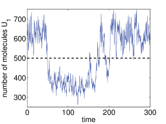
     (a)   (b)

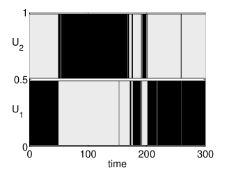
Figure 5: (a) The time evolution of $U_{1}$ computed for the generalized compartment-based model with $K_{u}=2$ and $K_{v}=1$. The homogeneous steady state $u_{s}^{2}=500$ is plotted using the dashed line. (b) The time-dependent pattern given by the values of $U_{1}$ and $U_{2}$ computed for the same realization of the Gillespie algorithm as in the panel (a).

3.2 Classical compartment-based model: $K_{u}=2$ and $K_{v}=2$

Next we consider the case where the whole interval $[0,\ L]$ is divided into two compartments for both $U$ and $V$. The discretization is illustrated in Figure 4(b). Denoting $u_{1}$, $u_{2}$, $v_{1}$ and $v_{2}$ the average numbers of molecules obtained by the corresponding mean-field model, they satisfy the following system of four ODEs Erban:2007:PGS

$$\frac{\mbox{d}u_{1}}{\mbox{d}t} = d_{u}(u_{2}-u_{1})+k_{1}h_{u}-k_{2}u_{1}+\frac{k_{4}}{h_{u}h_{v}}u_{1}^{2}v_{1},$$

$$\frac{\mbox{d}u_{2}}{\mbox{d}t} = d_{u}(u_{1}-u_{2})+k_{1}h_{u}-k_{2}u_{2}+\frac{k_{4}}{h_{u}h_{v}}u_{2}^{2}v_{2},$$

$$\frac{\mbox{d}v_{1}}{\mbox{d}t} = d_{v}(v_{2}-v_{1})+k_{3}h_{v}-\frac{k_{4}}{h_{u}^{2}}u_{1}^{2}v_{1},$$

$$\frac{\mbox{d}v_{2}}{\mbox{d}t} = d_{v}(v_{1}-v_{2})+k_{3}h_{v}-\frac{k_{4}}{h_{u}^{2}}u_{2}^{2}v_{2}.$$

Again letting the left hand side terms be zero and using $h_{u}=h_{v}=L/2$, we obtain the following system of algebraic equations

$$2d_{u}(u_{2}-u_{1})+k_{1}L-2k_{2}u_{1}+\frac{8k_{4}}{L^{2}}u_{1}^{2}v_{1} = 0,$$ (3.13)

$$2d_{u}(u_{1}-u_{2})+k_{1}L-2k_{2}u_{2}+\frac{8k_{4}}{L^{2}}u_{2}^{2}v_{2} = 0,$$ (3.14)

$$2d_{v}(v_{2}-v_{1})+k_{3}L-\frac{8k_{4}}{L^{2}}u_{1}^{2}v_{1} = 0,$$ (3.15)

$$2d_{v}(v_{1}-v_{2})+k_{3}L-\frac{8k_{4}}{L^{2}}u_{2}^{2}v_{2} = 0.$$ (3.16)

Adding all equations together, we have

$$u_{1}+u_{2}=\frac{(k_{1}+k_{3})L}{k_{2}}=2\omega L.$$ (3.17)

Adding (3.15) and (3.16), we also have

$$u_{1}^{2}v_{1}+u_{2}^{2}v_{2}=\frac{k_{3}L^{3}}{4k_{4}}=\frac{3\omega^{3}L^{3}}{4}.$$ (3.18)

Adding (3.13) and (3.15), we obtain

$$(k_{1}+k_{3})L-2k_{2}u_{1}+2d_{u}(u_{2}-u_{1})+2d_{v}(v_{2}-v_{1})=0.$$ (3.19)

Using (3.17), we have $u_{1}=(1+r)\omega L$ and $u_{2}=(1-r)\omega L$ for a suitable $r$. Thus (3.19) can be rewritten as

$$v_{2}-v_{1}=\frac{2r(1+d_{u})\omega L}{d_{v}}=2rR\omega L,$$ (3.20)

where we denoted $R=(1+d_{u})/d_{v}$. Substituting (3.20) into (3.15) and denoting $S=1+d_{u}=d_{v}R$, we have

$$v_{1}=\frac{(3+4Sr)\omega L}{8(1+r)^{2}}.$$ (3.21)

Similarly from (3.16) we have

$$v_{2}=\frac{(3-4Sr)L\omega}{8(1-r)^{2}}.$$ (3.22)

Substituting both (3.21) and (3.22) to (3.20), we obtain

$$\frac{3-4Sr}{8(1-r)^{2}}-\frac{3+4Sr}{8(1+r)^{2}}=2Rr.$$

which can be simplified to the equation

$$r\left(4R\left(1-r^{2}\right)^{2}+2S\left(1+r^{2}\right)-3\right)=0.$$

We are looking for the non-homogeneous solution where $r\neq 0$. Denoting $y=r^{2}>0$, we have a quadratic equation

$$4Ry^{2}+(2S-8R)y+(4R+2S-3)=0.$$ (3.23)

We will look for conditions such that the equation (3.23) has a solution $0<y<1$ (since $-1<r<1$). Let

$$f(y)=4Ry^{2}+(2S-8R)y+(4R+2S-3).$$ (3.24)

Then we have $f(1)=4S-3=1+4d_{u}>0$. One can verify that if $f(0)>0$, it is impossible for the equation $f(y)=0$ to have a solution between 0 and 1. On the other hand, if $f(0)<0$, we will definitely have a solution between 0 and 1. Thus we have a necessary and sufficient condition

$$f(0)=4R+2S-3<0,$$ (3.25)

which corresponds to the condition for $d_{u}$ and $d_{v}$:

$$\frac{4}{d_{v}}+2<\frac{3}{1+d_{u}}.$$

We note that $d_{u}=D_{u}/h^{2}$ and $d_{v}=D_{v}/h^{2}$, where $h=h_{u}=h_{v}=L/2$. Thus the necessary and sufficient condition for patterns becomes

$$\frac{L^{2}}{D_{v}}+2<\frac{3L^{2}}{L^{2}+4D_{u}}.$$ (3.26)

If $D_{v}\rightarrow\infty$, then the condition (3.26) becomes the condition (3.10) which was derived for the case of the generalized compartment-based model. The condition (3.10) is a necessary condition for (3.26) but not sufficient. We illustrate it in Figure 6 for $L=1$.

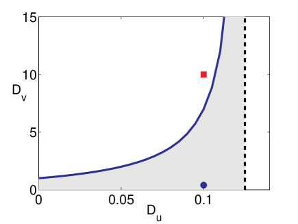
Figure 6: The regions of patterning in $D_{u}$-$D_{v}$ plane. The shaded area is the region where the standard compartment-based model does not yield patterns and the generalized compartment-based model has patterns. The (blue) circle is the parameter regime used in Figure 7(a) and the (red) square is the parameter regime used in Figure 7(b).

The condition (3.10) corresponds to all parameter values to the left of the dashed line in Figure 6. The condition (3.26) corresponds to the values of $D_{u}$ and $D_{v}$ which are above the (blue) solid line. The shaded area are parameter values for which the generalized compartment-based model yields non-homogeneous patterns and the standard compartment-based model does not. Next, we will use the same value of $D_{u}$ as in Figure 5, namely $D_{u}=0.1$. We choose two values of $D_{v}$ which are denoted as the (blue) circle and (red) square in Figure 6. We use the Gillespie algorithm to simulate the standard compartment-based model for $K_{u}=K_{v}=2$. The results are shown in Figure 7. The top panels show the time evolution of $U_{1}$ and $U_{2}$.

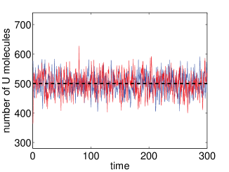
     (a)   (b)

        

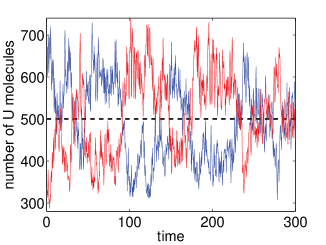
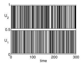
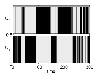
Figure 7: Time evolution of $U_{1}$ (blue line) and $U_{2}$ (red line) for $K_{u}=K_{v}=2$ is shown in top panels for (a) $D_{u}=0.1$, $D_{v}=0.4$ and (b) $D_{u}=0.1$, $D_{v}=10$. The corresponding time-dependent pattern is shown in bottom panels.

We clearly see the switching between two patterns for $D_{v}=10$, but there is no bistability for $D_{v}=0.4.$ The resulting patterns are visualized in the bottom panels. As in Figures 1, 3 and 5, we plot the values which are larger than the homogeneous steady state $u_{s}^{2}=500$ in black. Light gray colour denotes the values which are lower than $u_{s}^{2}=500$.

Let us note that we are comparing the generalized compartment-based model with $K_{u}=2$ and $K_{v}=1$ with the classical compartment-based model. In particular, the generalized compartment-based model uses $\gamma=2.$ If we substitute $\gamma=2$ in formula (2.10), we obtain $D_{v}=4D_{u}$. In particular, the parameter values $D_{u}=0.1$ and $D_{v}=0.4.$ are compatible with the choice (2.10). However, the standard comparment-based model does not exhibit patterns for this parameter choice as we observed in Figure 7(a).

Remark. Let $z=L^{2}$. Then the inequality (3.26) becomes

$$z^{2}+(4D_{u}-D_{v})z+8D_{u}D_{v}<0,$$ (3.27)

which is possible for some values of $L$ if and only if

$$4D_{u}<D_{v}\quad\mbox{and}\quad(4D_{u}-D_{v})^{2}-32D_{u}D_{v}>0.$$ (3.28)

Thus patterns are possible for some values of $L$ provided that

$$\frac{D_{v}}{D_{u}}>20+8\sqrt{6}\approx 39.6.$$ (3.29)

This condition is also the condition for the Turing patterns to show for the original system of mean-field partial differential equations (2.2)–(2.3).

4 Comparison of compartment-based models for $K_{u}>2$

The condition (3.10) for the generalized compartment-based model is only a necessary condition for the condition (3.26) for the classical case as we showed in Figure 6. The bistability condition difference suggests that, if we use different discretizations for $U$ and $V$, the stability of the homogeneous system may change. In this section, we compare the generalized and classical compartment-based models for $K_{u}>2.$ In Figure 8, we use $D_{u}=5\times 10^{-4}$ and $D_{v}=20D_{u}$. In this case the condition for (deterministic) Turing patterns (3.29) is not satisfied. The classical compartment-based model also does not show Turing patterns as it is demonstrated in Figure 8(a) (with $K_{u}=K_{v}=64$ compartments) and Figure 8(b) (with $K_{u}=K_{v}=8$ compartments). In both cases, no spatial Turing pattern is observed except noise from stochastic effect. However, if the generalized compartment-based model is used, then the Turing pattern may appear. In Figure 8(c), a result for the generalized compartment-based model with $K_{u}=64$ and $K_{v}=8$ is presented. There is a clear Turing pattern. In Figure 8(c), we have $\gamma=8$. We also tested cases when $\gamma=2$ and $\gamma=4$ and obtained Turing patterns. The case $\gamma=4$ is plotted in Figure 8(d).

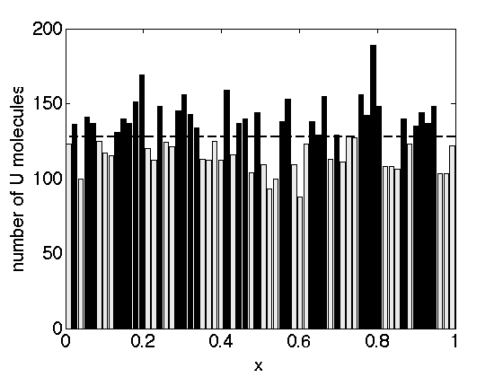
     (a)   (b)

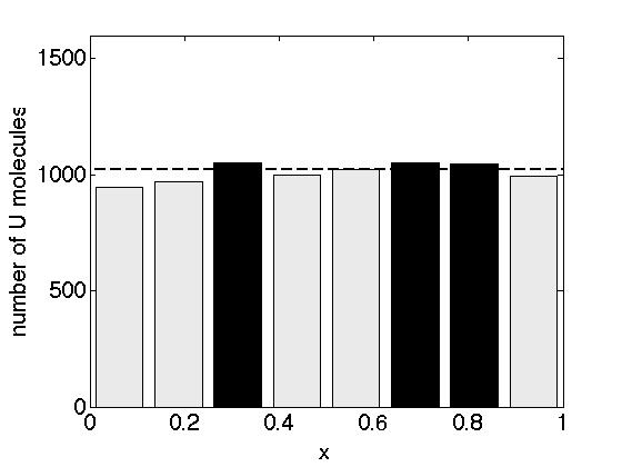
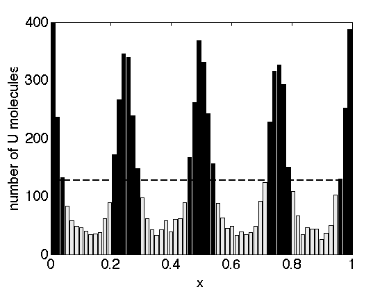
     (c)   (d)

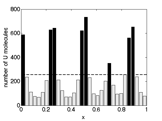
Figure 8: Spatial distribution of $U$ at time $T=100$ for $D_{v}=20D_{u}$, $\omega=4096$ and $D_{u}=5\times 10^{-4}$ with (a) $K_{u}=K_{v}=64$; (b) $K_{u}=K_{v}=8$; (c) $K_{u}=64$ and $K_{v}=8$; (d) $K_{u}=32$ and $K_{v}=8$. There is no Turing pattern in the top panels (classical compartment-based model). Turing patterns appear in the bottom panels (generalized compartment-based model).

In Figure 9, we demonstrate that both discretizations strategies clearly show Turing patterns when we increase the ratio of diffusion constants to $D_{v}/D_{u}=80$. In this case, the condition for (deterministic) Turing patterns (3.29) is satisfied. Finally, we present results for $D_{v}=40D_{u}$ in Figure 10. In the deterministic PDE system, when $D_{v}=40D_{u}$, Turing pattern should still appear. But in the classical compartment-based model, it is hard to claim that there is a visible Turing pattern (see Figures 10(a) and 10(c)). Considering the generalized compartment-based model, Turing patterns can be clearly observed (see Figures 10(b) and 10(d)).

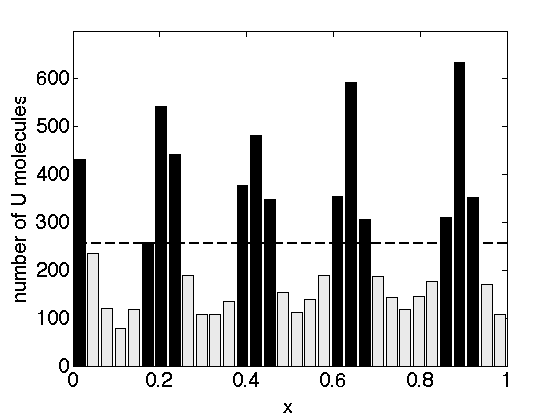
     (a)   (b)

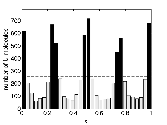
Figure 9: Spatial distribution of $U$ at time $T=100$ for $D_{v}=80D_{u}$. Both discretization strategies clearly show Turing patterns. We use $\omega=4096$, $D_{u}=5\times 10^{-4}$ with (a) $K_{u}=K_{v}=32$; (b) $K_{u}=32$ and $K_{v}=8$.

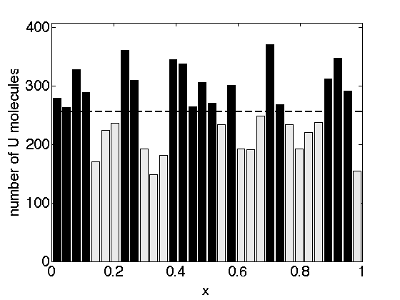
     (a)   (b)

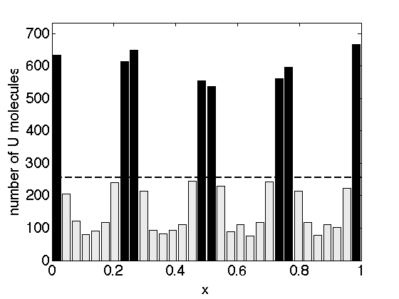
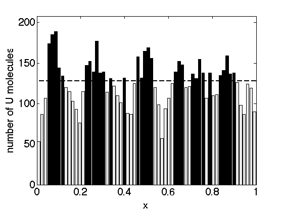
     (c)   (d)

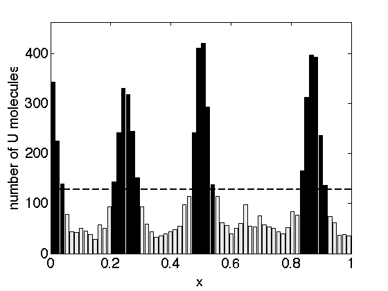
Figure 10: Spatial distribution of $U$ at time $T=100$ for $D_{v}=40D_{u}$. The generalized compartment-based model clearly shows Turing patterns, while it is difficult to see whether Turing patterns appear in the classical compartment-based model. We use $\omega=4096$, $D_{u}=5\times 10^{-4}$ with (a) $K_{u}=K_{v}=32$; (b) $K_{u}=32$ and $K_{v}=8$; (c) $K_{u}=K_{v}=64$; (d) $K_{u}=64$ and $K_{v}=8$.

5 Discussion

We showed that two choices of compartments illustrated in Figure 2 can give different parameter regions for stochastic Turing patterns. An obvious question is which one is correct. One possibility to address this question is to consider a more detailed molecular-based approach which would be written in the form of Brownian dynamics Erban:2009:SMR . We are currently working on such a simulation and we will report our findings in a future publication.

Although our results might look like a warning against the use of compartment-based methods for patterns based on the Turing mechanism, there are very good reasons to use the compartment-based model in other situations Engblom:2009:SSR ; Isaacson:2006:IDC . Compartment-based models are often less computationally intensive than detailed Brownian dynamics simulations Flegg:2012:TRM ; Hellander:2012:CMM . They can be used for developing efficient multiscale methods where parts of the domain are simulated using the detailed Brownian dynamics while the rest of the domain is simulated using compartments Erban:2013:MRS ; Flegg:2013:DSN . They can also be used to bridge Brownian dynamics simulations with macroscopic PDEs Ferm:2010:AAS , because direct multiscale methods for coupling Brownian dynamics with PDEs are challenging to implement Franz:2013:MRA .

We showed in Figure 9 that the resulting patterns are comparable when the ratio of diffusion constants is sufficiently large. In this case, the generalized compartment-based model could also be used to construct computational approaches to speed-up simulations of the standard compartment-based model, because it does not simulate all diffusion events for chemical species with large diffusion constants LiCao2012 ; LiCao2013 .

References

- (1) M. Asslani, F. Di Patti, and D. Fanelli. Stochastic Turing patterns on a network. Physical Review E, 86:046105, 2012.
- (2) I. Barrass, E. Crampin, and P. Maini. Mode transitions in a model reaction-diffusion system driven by domain growth and noise. Bulletin of Mathematical Biology, 68:981–995, 2006.
- (3) T. Biancalani, D. Fanelli, and F. Di Patti. Stochastic Turing patterns in a Brusselator model. Physical Review E, 81:046215, 2010.
- (4) T. Biancalani, T. Galla, and A. McKane. Stochastic waves in a Brusselator model with nonlocal interaction. Physical Review E, 84:026201, 2011.
- (5) A. Black and A. McKane. Stochastic formulations of ecological models and their applications. Trends in Ecology and Evolution, 27(6):337–345, 2012.
- (6) T. Butler and N. Goldenfeld. Fluctuation-driven Turing patterns. Physical Review E, 84:011112, 2011.
- (7) Y. Cao, H. Li, and L. Petzold. Efficient formulation of the stochastic simulation algorithm for chemically reacting systems. Journal of Chemical Physics, 121(9):4059–4067, 2004.
- (8) E. Crampin, E. Gaffney, and P. Maini. Reaction and diffusion on growing domains: Scenarios for robust pattern formation. Bulletin of Mathematical Biology, 61:1093–1120, 1999.
- (9) S. Engblom, L. Ferm, A. Hellander, and P. Lötstedt. Simulation of stochastic reaction-diffusion processes on unstructured meshes. SIAM Journal on Scientific Computing, 31:1774–1797, 2009.
- (10) R. Erban and S. J. Chapman. Reactive boundary conditions for stochastic simulations of reaction-diffusion processes. Physical Biology, 4(1):16–28, 2007.
- (11) R. Erban and S. J. Chapman. Stochastic modelling of reaction-diffusion processes: algorithms for bimolecular reactions. Physical Biology, 6(4):046001, 2009.
- (12) R. Erban, S. J. Chapman, and P. Maini. A practical guide to stochastic simulations of reaction-diffusion processes. 35 pages, available as http://arxiv.org/abs/0704.1908, 2007.
- (13) R. Erban, M. Flegg, and G. Papoian. Multiscale stochastic reaction-diffusion modelling: application to actin dynamics in filopodia. Bulletin of Mathematical Biology, to appear:DOI: 10.1007/s11538–013–9844–3, 2013.
- (14) D. Fange and J. Elf. Noise-induced Min phenotypes in E. coli. PLoS Computational Biology, 2(6):637–648, 2006.
- (15) L. Ferm, A. Hellander, and P. Lötstedt. An adaptive algorithm for simulation of stochastic reaction-diffusion processes. Journal of Computational Physics, 229:343–360, 2010.
- (16) M. Flegg, J. Chapman, and R. Erban. The two-regime method for optimizing stochastic reaction-diffusion simulations. Journal of the Royal Society Interface, 9(70):859–868, 2012.
- (17) M. Flegg, S. Rüdiger, and R. Erban. Diffusive spatio-temporal noise in a first-passage time model for intracellular calcium release. Journal of Chemical Physics, 138:154103, 2013.
- (18) B. Franz, M. Flegg, J. Chapman, and R. Erban. Multiscale reaction-diffusion algorithms: PDE-assisted Brownian dynamics. SIAM Journal on Applied Mathematics, 73(3):1224–1247, 2013.
- (19) Z. Fu, X. Xu, H. Wang, and Q. Quoyang. Stochastic simulation of Turing patterns. Chinese Physical Letters, 25(4):1220–1223, 2008.
- (20) M. Gibson and J. Bruck. Efficient exact stochastic simulation of chemical systems with many species and many channels. Journal of Physical Chemistry A, 104:1876–1889, 2000.
- (21) D. Gillespie. Exact stochastic simulation of coupled chemical reactions. Journal of Physical Chemistry, 81(25):2340–2361, 1977.
- (22) J. Hattne, D. Fange, and J. Elf. Stochastic reaction-diffusion simulation with MesoRD. Bioinformatics, 21(12):2923–2924, 2005.
- (23) A. Hellander, S. Hellander, and P. Lötstedt. Coupled mesoscopic and microscopic simulation of stochastic reaction-diffusion processes in mixed dimensions. Multiscale Modeling and Simulation, 10(2):585–611, 2012.
- (24) S. Hellander, A. Hellander, and L. Petzold. Reaction-diffusion master equation in the microscopic limit. Physical Review E, 85:042901, 2012.
- (25) Y. Hori and S. Hara. Noise-induced spatial pattern formation in stochastic reaction-diffusion systems. Proc. of 51st IEEE Conference on Decision and Control, pages 1053–1058, 2012.
- (26) J. Hu, H. Kang, and H. Othmer. Stochastic analysis of reaction-diffusion processes. Bulletin of Mathematical Biology, to appear:DOI: 10.1007/s11538–013–9849–y, 2013.
- (27) S. Isaacson. The reaction-diffusion master equation as an asymptotic approximation of diffusion to a small target. SIAM Journal on Applied Mathematics, 70(1):77–111, 2009.
- (28) S. Isaacson and C. Peskin. Incorporating diffusion in complex geometries into stochastic chemical kinetics simulations. SIAM Journal on Scientific Computing, 28(1):47–74, 2006.
- (29) H. Kang, L. Zheng, and H. Othmer. A new method for choosing the computational cell in stochastic reaction-diffusion systems. Journal of Mathematical Biology, 65(6-7):1017–1099, 2012.
- (30) P. Kepper, V. Castets, E. Dulos, and J. Boissonade. Turing-type chemical patterns in the chlorite-iodide-malonic acid reaction. Physica D, 49:161–169, 1991.
- (31) F. Li and Y. Cao. Multiscale discretization for reaction diffusion systems. Proceedings of the 2012 International Conference on Bioinformatics and Computational Biology (Editors: Hamid R. Arabnia, Quoc-Nam Tran Associate Editors: Andy Marsh, Ashu M. G. Solo), Las Vegas, Nevada, USA, 2012, 305-311.
- (32) F. Li and Y. Cao. Optimal discretization size and multigrid discretization method for 1D multiscale reaction diffusion systems. submitted.
- (33) P. Maini, T. Woolley, R. Baker, E. Gaffney, and S. Seirin Lee. Turing’s model for biological pattern formation and the robustness problem. Interface focus, 2:487–496, 2012.
- (34) A. McKane, T. Biancalani, and T. Rogers. Stochastic pattern formation and spontaneous polarization: the linear noise approximation and beyond. Bulletin of Mathematical Biology, to appear:DOI: 10.1007/s11538–013–9827–4, 2013.
- (35) J. Murray. Mathematical Biology. Springer Verlag, 2002.
- (36) L. Qiao, R. Erban, C. Kelley, and I. Kevrekidis. Spatially distributed stochastic systems: Equation-free and equation-assisted preconditioned computation. Journal of Chemical Physics, 125:204108, 2006.
- (37) Q. Quyang and H. Swinney. Transition from a uniform state to hexagonal and striped Turing patterns. Nature, 352:610–612, 1991.
- (38) R. Satnoianu, M. Menzinger, and P. Maini. Turing instabilities in general systems. J. Math. Biol., 41:493–512, 2000.
- (39) J. Schnakenberg. Simple chemical reaction systems with limit cycle behaviour. Journal of Theoretical Biology, 81:389–400, 1979.
- (40) M. Scott, F. Poulin, and H. Tang. Approximating intrinsic noise in continuous multispecies models. Proceedings of the Royal Society A, 467:718–737, 2011.
- (41) S. Sick, S. Reinker, J. Timmer, and T. Schlake. WNT and DKK determine hair follicle spacing through a reaction-diffusion mechanism. Science, 314:1447–1450, 2006.
- (42) A. Turing. The chemical basis of morphogenesis. Phil. Trans. Roy. Soc. Lond., 237:37–72, 1952.
- (43) A. Twomey. On the stochastic modelling of reaction-diffusion processes. M.Sc. Thesis, University of Oxford, United Kingdom, September 2007.
- (44) M. Vigelius and B. Meyer. Stochastic simulations of pattern formation in excitable media. PLoS ONE, 7(8):e45208, 2012.
- (45) T. Woolley, R. Baker, E. Gaffney, and P. Maini. Power spectra methods for a stochastic description of diffusion on deterministically growing domains. Physical Review E, 84:021915, 2011.
- (46) T. Woolley, R. Baker, E. Gaffney, and P. Maini. Stochastic reaction and diffusion on growing domains: understanding the breakdown of robust pattern formation. Physical Review E, 84:046216, 2011.
- (47) T. Woolley, R. Baker, E. Gaffney, P. Maini, and S. Seirin-Lee. Effects of intrinsic stochasticity on delayed reaction-diffusion patterning systems. Physical Review E, 85:051914, 2012.