Stellar feedback by radiation pressure and photoionization

Abstract

The relative impact of radiation pressure and photoionization feedback from young stars on surrounding gas is studied with hydrodynamic radiative transfer (RT) simulations. The calculations focus on the single-scattering (direct radiation pressure) and optically thick regime, and adopt a moment-based RT-method implemented in the moving-mesh code arepo. The source luminosity, gas density profile and initial temperature are varied. At typical temperatures and densities of molecular clouds, radiation pressure drives velocities of order $\sim 20\,\rm km\,s^{-1}$ over $1$-$5\,\rm Myr$; enough to unbind the smaller clouds. However, these estimates ignore the effects of photoionization that naturally occur concurrently. When radiation pressure and photoionization act together, the latter is substantially more efficient, inducing velocities comparable to the sound speed of the hot ionized medium ($10$-$15\,\rm km\,s^{-1}$) on timescales far shorter than required for accumulating similar momentum with radiation pressure. This mismatch allows photoionization to dominate the feedback as the heating and expansion of gas lowers the central densities, further diminishing the impact of radiation pressure. Our results indicate that a proper treatment of the impact of young stars on the interstellar medium needs to primarily account for their ionization power whereas direct radiation pressure appears to be a secondary effect. This conclusion may change if extreme boosts of the radiation pressure by photon trapping are assumed.

1 Introduction

Massive stars can dramatically change the environment in which they are born. Although the most profound transformation awaits their final explosion as supernova, their impact on the surrounding gas starts much earlier, mediated by their ionizing radiation. Shortly after young stars start shining, the emitted photons ionize the surrounding media, burning hot ionized bubbles into the otherwise cold neutral gas. The production of these HII regions has interesting consequences not only for the structure and the dynamics of the gas at scales of clouds and the interstellar medium (ISM), but potentially also on much larger galactic/halo scales. The overall importance of these effects depends strongly on the efficiency with which radiation couples to the gas, the subject studied in this paper.

Photons carry energy $E=h\nu$ and momentum $P=h\nu/c$, where $h$ is Planck’s constant, $\nu$ the photon frequency and $c$ the speed of light. Both quantities are conserved during photon-atom interactions. The photon’s energy can change the ionization state of an atom and produce heat through the thermalization of the left-over energy above the ionization threshold (e.g. energy above $E_{0}=13.6\,\rm eV$ for the case of a neutral hydrogen atom initially in the ground state). The photon’s momentum will be transferred to the atom too, which thus receives a velocity kick in the direction of the absorbed photon.

Young massive stars emit mostly in the UV region of the spectrum, with a frequency averaged mean energy $\left<E\right>\sim 20\,\rm eV$. This is enough to ionize the neutral gas and also to heat it up to temperatures $T\sim 10^{4}\,{\rm K}$. The hot bubbles produced around stars – the HII regions – are then hotter than the surrounding medium, which is characterized by temperatures $T\sim 10^{2}\,\rm K$ and below. These temperature differences create pressure imbalances, resulting in a net acceleration of the gas (see Chapter 20, Shu, 1992, for a detailed description). This process, here collectively referred to as “photoionization”, can induce significant radial velocities in the gas away from the heating sources. Early analytical calculations and more recent numerical simulations have confirmed the importance of photoionization for the dynamics of molecular clouds (Whitworth, 1979; McKee et al., 1984; McKee, 1989; Matzner, 2002; Dale et al., 2005; Krumholz et al., 2006; Dale et al., 2012; Walch et al., 2012).

However, the momentum of the photon is also conserved. An atom of mass $m$ will receive an additional velocity kick $\Delta V=E/(c\;m)$ per absorption of a photon with energy $E$, independent of the global effects induced by photoionization. The extra momentum acts like a pressure force and is commonly referred to as “radiation pressure”. We can make a simple estimate of this effect in the case of an optically thick shell of gas in the presence of an ionizing source with luminosity $L$. The optically thick regime guarantees that all photons are absorbed at the edge of the shell, which will hence increase its momentum $P$ according to (Murray et al., 2005):

$$\frac{{\rm d}P}{{\rm d}t}=\frac{GM(r)M_{g}(r)}{r^{2}}+\frac{L}{c},$$ (1)

where $M$ and $M_{g}$ are the total enclosed mass and gas mass, respectively. If one ignores the effects of gravity described by the first term on the right hand side in Eq. (1), the velocity of the gas can be written as:

$$V_{\rm shell}=\frac{L\;t}{c\;M_{\rm shell}}$$ (2)

where $M_{\rm shell}$ is the mass of the shell, which will in general depend on the underlying density distribution. In the case of a uniform gas density, $\rho_{0}$, the velocity induced in the gas will be (Wise et al., 2012):

$$V_{\rm shell}=tA(r_{i}^{4}+2At^{2})^{-3/4}$$ (3)

where $A=3L/4\rm\pi\rho_{0}c$ and $r_{i}$ is the initial position of the shell. Wise et al. (2012) argue that the shell will first form when ionizations balance recombinations at the Strömgren radius, then $r_{i}=r_{s}=(3\dot{N}_{\gamma}/4\rm\pi\alpha_{B}(n_{H})^{2})^{1/3}$, where $\dot{N}_{\gamma}$ is the emission rate of photons, $n_{\rm H}$ the hydrogen number density and $\alpha_{\rm B}$ the case-B recombination coefficient (Dopita & Sutherland, 2003).

Using typical values for the emission of young massive stars, the arguments above suggest that radiation pressure alone could drive winds reaching a few hundred $\rm km\,s^{-1}$ (Murray et al., 2005; Sharma et al., 2011; Hopkins et al., 2011; Wise et al., 2012). Also, radiation pressure from a central AGN could be relevant (e.g. Haehnelt, 1995) too. It is also noteworthy that momentum cannot be radiated away, unlike energy in the form of heat, a property that might be beneficial in numerical simulations where lack of numerical resolution can artificially boost radiative cooling losses. These factors have stimulated a significant interest in the galaxy formation community in radiation pressure as an alternative to thermal supernova feedback for regulating star formation and, in particular, for driving galactic winds.

Because of the technical challenges of including radiative transfer calculations within galaxy-scale simulations, the effects of radiation pressure have often been included in a “sub-grid” fashion that attempts to approximate the radiation transport effects (however, see Wise et al., 2012; Kim et al., 2013). The accuracy of these recipes depends heavily on the particular assumptions and approximations made in each model, and thus it is perhaps not surprising that the reported results for radiation pressure effects vary considerably, from helping to regulate star formation (Wise et al., 2012; Agertz et al., 2013) to driving galactic scale winds that remove gas from the galaxies out the halo and beyond (Oppenheimer & Davé, 2006; Aumer et al., 2013; Ceverino et al., 2013).

In part, these large differences are rooted in varying assumptions about the effect of radiation trapping by dust. Dust grains can absorb photons and re-emit them in the infrared, making more photons available for absorptions. This “boosts” the effect of radiation pressure by a factor $\tau=\kappa_{\rm IR}\Sigma_{\rm gas}$, which depends on the dust opacity $\kappa_{\rm IR}$ and the gas column density $\Sigma_{\rm gas}$. There is no clear consensus on realistic values for $\tau$; under normal galaxy conditions, some authors have argued in favor of values in the range $0-30$ (Hopkins et al., 2011, and references therein). Strictly speaking, we note that this mechanism can however not be regarded as direct momentum driving any more since it depends on the absorption of photons with a given energy $E$ and their re-radiation, having no link with the momentum $E/c$ originally carried by the source photons (Krumholz & Matzner, 2009). In this paper, we will not consider radiation trapping but concentrate on the momentum-driven feedback given by the interaction of the gas with the momentum content of each photon. This is sometimes referred to as the “single-scattering” regime.

Massive stars not only emit significant amounts of radiation but they also deposit energy into their surroundings via stellar winds, whose energy accumulated during the lifetime of the star can match that of the final supernova explosions (Castor et al., 1975). Recent studies suggest that stellar winds can have a sizable impact on the structure of clouds (Harper-Clark & Murray, 2009; Rogers & Pittard, 2013), albeit the rate at which they modify the dynamics might be slow (Dale & Bonnell, 2008). Analytical estimates of the total energy budget deposited by massive stars suggest that radiation will dominate over the input from winds (Matzner, 2002), with stellar population models suggesting a factor $\sim 100$ higher energy deposition in radiation than the expected from supernova explosions (Agertz et al., 2013). Determining the efficiency with which this energy couples to the surrounding gas is therefore fundamental to understand the very nature of stellar feedback.

A proper treatment of radiation-induced winds in galaxies requires a close look at the physical scales of a few $\rm pc$ typical of stellar HII regions. The problem is challenging not only because of the large dynamic range of scales involved, but also because it requires an appropriate treatment of the radiation transport and its coupling to the dynamics of the gas. Most of the recent progress in this area has been made by analytical studies, which suggest that radiation pressure is small compared to the gas pressure by photoionization (e.g. Mathews, 1969; Gail & Sedlmayr, 1979; Arthur et al., 2004). However, this might not be true for more luminous stars embedded in massive molecular clouds (Krumholz & Matzner, 2009). Studying the problem with numerical simulations is attractive because such studies account for spatially resolved details normally not considered in the analytical treatments (which usually relate to the behaviour of a “shell” or radius of interest). Also, numerical simulations can naturally follow the non-linear coupling between the radiation, the dynamics of the gas, and the gravitational field created by the total mass distribution. Here we take a step in this direction.

We present a series of controlled numerical simulations with radiative transfer of idealized set-ups, with a central ionizing source embedded in an initially neutral gaseous medium composed of hydrogen. We compare the effects of photoionization and radiation pressure in optically-thick gas under two configurations: $i)$ a constant density media and $ii)$ an isothermal density profile. The paper is organized as follows: our code and radiative transfer implementation are described in Section 2, the effects of radiation on the gas are examined in Section 3 and  4. We discuss and compare our findings with previous work in Section 5 and conclude by highlighting our most important results. Additional radiative transfer tests and convergence studies are presented in the Appendices.

2 Numerical Simulations with Radiative Transfer

In our simulations we use the arepo code (Springel, 2010) to which we have added a moment-based radiative transfer (RT) module inspired largely by the scheme presented in Petkova & Springel (2009, hereafter PS09). In the following, we briefly describe the main characteristics of the code. We refer the reader to the original papers for further details.

2.1 Hydrodynamics and gravity

arepo uses an unstructured moving mesh to discretize and solve the hydrodynamic Euler equations. The mesh is defined as the Voronoi tessellation of the computational domain resulting from a set of mesh-generating points which are allowed to move freely and follow the local flow velocity. The fluxes across cells are computed with a second-order accurate Godunov scheme with an exact Riemann solver. A method for on-the-fly refinement and de-refinement of cells can be invoked to ensure, for example, that fluid cells have masses that do not differ by more than a factor of $\sim 2$ from a target mass resolution (Vogelsberger et al., 2012). The mesh is updated every timestep, and the geometry of cells is regularized mildly by adding small steering velocities to the mesh generating point where needed. A reasonably regular Voronoi mesh reduces reconstruction errors and allows larger timesteps, it is hence beneficial for the performance and accuracy of the code. These features allow arepo to follow complex flows in a highly adaptive quasi-Lagrangian manner, and in a fully Galilean-invariant way where bulk velocities do not introduce additional advection errors. The performance and suitability of the code to handle standard fluid problems has been analyzed in several previous works (Springel, 2010; Sijacki et al., 2012; Bauer & Springel, 2012; Muñoz et al., 2013).

The gravity solver is based on a TreePM scheme where forces are split into short- and long-range components, offering a uniformly high force accuracy and full adaptivity. The backbone of the solver is the same as in the widely used GADGET-2 code (Springel, 2005). Despite its novel character, arepo has already been used to tackle a range of astrophysical problems inherent to galaxy formation and first star formation (Vogelsberger et al., 2013; Nelson et al., 2013; Torrey et al., 2014; Marinacci et al., 2014; Pakmor & Springel, 2013; Bird et al., 2013, among others).

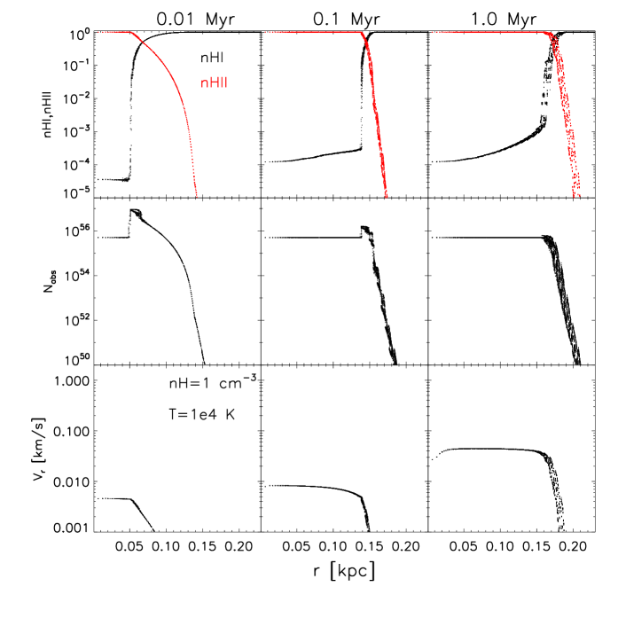
Figure 1: Several quantities of interest in our experiment with a constant density box, $n_{\rm H}=1\,\rm cm^{-3}$, fixed temperature $T=10^{4}\,\rm K$ and a central source with luminosity $L=10^{6}\,L_{\odot}$. Upper row: Time evolution of the ionization front in a thin slab around the source. Dots correspond to individual cells, and black and red indicate the fraction of neutral and ionized gas, respectively. Middle row: Number of photons absorbed in a given time-step (arbitrary units). Absorptions occur preferentially near the edge of the ionized region at early times but are distributed uniformly within the Strömgren sphere after the recombination time is reached; $t_{\rm rec}\sim 0.125\,\rm Myr$ for this set up. Bottom row: Velocity profiles of the gas due to radiation pressure. Momentum is deposited only within the ionized sphere.

2.2 The radiative transfer module

We have implemented in arepo a new version of the radiative transfer module introduced in PS09 and originally developed for gadget. The structural similarity of both codes allowed a relatively straightforward adaptation with only a small number of changes.

Briefly, we solve the moments of the radiative transfer equation using the Eddington tensor approximation as a closure relation. The Eddington tensor is estimated under an optically thin approximation, following the ideas of the optically-thin variable Eddington tensor (OTVET) approach of Gnedin & Abel (2001). More specifically, the code solves the following equation:

$$\frac{\partial J_{\nu}}{\partial t}=\frac{c}{a^{2}}\frac{\partial}{\partial x_{j}}\left(\frac{1}{\hat{\kappa}_{\nu}}\frac{\partial J_{\nu}h^{ij}}{\partial x_{i}}\right)-c\hat{\kappa}_{\nu}J_{\nu}+cj_{\nu},$$ (4)

where $J_{\nu}$ is the mean intensity, $a$ the expansion factor (for cosmological runs), $j_{\nu}$ the emission coefficient and $\hat{\kappa_{\nu}}$ the comoving absorption coefficient. $h^{ij}$ is the Eddington tensor, which is related to the third moment of the radiation intensity, the radiation pressure $P^{ij}_{\nu}$, through the relation $P^{ij}_{\nu}=J_{\nu}h^{ij}$. Eq. (4) describes the evolution of the intensity of the radiation field at a given point due to photon-conserving radiation transport via anisotropic diffusion (first term right hand side), and the influence of source and sink terms that are described by the absorption and emissivity terms on the right hand side.

Solving this equation requires the knowledge of the Eddington tensor, which is, a-priori unknown. Following Gnedin & Abel (2001), we invoke an optically-thin approximation to compute the tensor, which in practice involves an inverse distance square law to all sources, similar to gravity. This approximation neglects possible absorptions occurring in between the sources and the cell of interest, but it is in most situations good enough to define the primary direction of photon propagation accurately. For instance, in the case of a single source (e.g. a star), the corresponding dominant eigenvector of the Eddington tensor points radially away from the location of the star, as expected for photons streaming freely from a central source (see also Fig. 11).

Originally, PS09’s numerical implementation of the method was designed to work with an SPH framework, with the discretization scheme and numerical solvers chosen accordingly (see Sec. 4 in PS09). We have adapted the techniques to our moving-mesh approach with a deliberately minimum number of changes in the radiative transfer scheme. In arepo, the information for each cell can be associated with the mesh-generating points, allowing them to be interpreted as the corresponding quantities for a fiducial SPH particle, facilitating the task. We only need to introduce the concept of a smoothing length $h$ to AREPO (which is otherwise unnecessary) such that kernel interpolants can be defined in the same way as done in SPH codes like gadget. Once the smoothing lengths are computed by searching for the closest 64 neighboring mesh-generating points (which represent the cells), we follow the exact same discretized equations for radiative transfer as proposed originally in PS09.

For the time integration of the radiative transfer equation, we adopt an implicit scheme which is solved with an iterative conjugate-gradient method, ensuring stability of the diffusion problem and conservation of photon number. A flux-limiter $\lambda$ enforces the condition of sub-luminal transport of photons when the intensity gradients are large. The flux-limited diffusion version of the scheme is obtained by adding $\lambda$ as a multiplicative factor within the parenthesis of the first term on the right-hand side of Eq. (4). Based on carrying out several tests problems, we found that a flux-limiter of the form proposed by Levermore & Pomraning (1981) provides accurate results (see Appendix A). In arepo we then use:

$$\lambda=\frac{2R}{6+3R+R^{2}},$$ (5)

where $R=|\nabla n_{\gamma}|/(\kappa\,n_{\gamma})$ and $n_{\gamma}$ gives the number density of photons. We use the same chemical network described in PS09 to track the changes in ionization state of the gas.

The code can be used in a mono- or multi-frequency mode; in the latter, the emission is approximated by a black-body spectrum of a given temperature $T_{\rm BB}$, and decomposed in four different frequency bins with boundaries $\nu=[13.6,~{}24.4,~{}54.4,~{}70.0]\,{\rm eV}$. In the multi-frequency mode, Eq. (4) is solved independently for each bin, accounting for different absorption cross-sections, photon densities and opacities per bin. The code handles a mixture of hydrogen and helium gas, but for simplicity we use pure hydrogen in our experiments below.

2.3 Photoionization and radiation pressure

The temperature of the gas is followed by considering several mechanisms of cooling and heating. The treatment of cooling includes processes such as recombination cooling, collisional ionization cooling, collisional excitation cooling and Bremsstrahlung cooling. All rates are taken from Cen (1992) and are summarized in the Appendix A of PS09.

For hydrogen-only gas, irradiated by a source of photons with frequency $\nu$, the photoheating rate is given by

$$\Gamma=n_{\rm HI}\int{\rm d}\Omega\int_{\nu_{o}}^{\infty}{\rm d}\nu\,\frac{I_{\nu}\sigma_{\nu}}{h\nu}(h\nu-h\nu_{o}),$$ (6)

where $\rm d\Omega$ is the differential solid angle and $\sigma_{\nu}$ gives the absorption cross-section at frequency $\nu$.

Notice that a source emitting photons at exactly the ionization frequency, $\nu=\nu_{0}$, will not produce any heating in the gas. However, photoheating becomes important when harder photons are considered. For the conditions used in our experiments, heating will always dominate over cooling.

The temperature changes resulting from ionizing radiation can produce pressure gradients, inducing net motions of the gas. Note that our radiative transfer scheme is fully coupled to the hydrodynamical solver which guarantees a self-consistent update of the gas dynamics due to photoionization.

By means of the radiative transfer module, we track the number of photon absorptions per cell, allowing the computation of the momentum deposition into gas by radiation of energy $E$ as:

$$\Delta V_{\rm cell}=\frac{N_{\rm abs}\,E}{c\;m_{\rm cell}},$$ (7)

where $\Delta V_{\rm cell}$ is the modulus of the velocity kick given to a cell with mass $m_{\rm cell}$ that absorbs a net number of photons $N_{\rm abs}$ in a given time-step. The kick is directed radially outwards from the source.

The radiative transfer module is robust to changes in time-step and smoothing lengths. It takes full advantage of the gravity-tree structure to compute the Eddington tensor, minimizing the introduced overhead. The strongest advantage of this approach, not really exploited in this work, is its independence from the number of sources, making it especially useful for applications where this number is large, such as cosmic reionization. On the other hand, being a photon diffusion scheme, shadows are not cast properly, compromising the accuracy when this is important. To check our implementation, we have carried out the set of standard radiative transfer tests suggested in Iliev et al. (2006, 2009), obtaining satisfactory results. We summarize the tests in Appendix A.

Table 1: Summary of properties for constant density runs. Columns show the density, temperature, side length of the box, Strömgren radius and recombination time. All numerical experiments were initialized with $64^{3}$ cells. The central source emits with luminosity $L=10^{6}\,\rm L_{\odot}$.

$n_{\rm H}$	$T$	$L_{\rm box}$	$r_{s}$	$t_{\rm rec}$
$[\rm cm^{-3}]$	[K]	[pc]	[pc]	[$10^{3}\,\rm yr$]
0.1	$10^{4}$	4000	808.2	1218.3
1.0	$10^{2}$	200	47.4	2.43
1.0	$10^{4}$	700	174.4	121.83
50	$10^{4}$	50	12.88	2.44
100	$10^{2}$	9	2.20	0.024
100	$10^{4}$	30	8.12	1.22

3 Radiation pressure in a constant density medium

3.1 Radiation pressure acting alone

Our first series of experiments investigates the effect of radiation pressure in gas at constant density $n_{\rm H}$ and temperature $T$. Table 1 summarizes the different initial conditions, where we have adjusted the length of the box to keep the resolution fixed in units of the local Strömgren sphere. At $t=0$, the gas is fully neutral, and we switch on a central source of ionizing photons with luminosity $L=10^{6}\,L_{\odot}\simeq 1.8\times 10^{50}\,\rm photons/s$. For simplicity, in this Section we will first assume that all photons are emitted at the hydrogen ionization energy $E_{0}=13.6\;\rm eV$. This maximizes the number of ionizations at a given luminosity, and therefore, the deposition of momentum into the gas (see Sec. 4 for a different source spectral shape). Notice that the assumption of a monochromatic source at $E_{0}$ means that there are no heating sources due to radiation in these runs and therefore the internal energy per unit mass of the cells, $u$, experiences no change due to the presence of a luminous source. This translates into an approximately constant temperature in the cells, besides a reduction by a factor of 2 due to the change in molecular weight of ionized hydrogen ($T\propto\mu u$). Although this is a very special set-up, it highlights in a clean way the effects of the different variables at play.

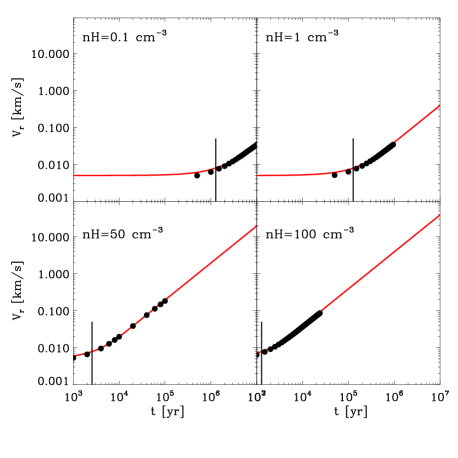
Figure 2: Velocity of the gas measured in simulations with different densities, $n_{\rm H}=0.1$, $1$, $50$, and $100\,\rm cm^{-3}$, fixed temperature $T=10^{4}\,\rm K$ and luminosity $L=10^{6}\,L_{\odot}$, as a function of time (black dots). $V_{r}$ corresponds to the mass-weighted radial velocity within the instantaneous ionization radius $r_{\rm ion}$. The behaviour is well described by simple analytical arguments (red lines) where $V_{r}=L/(c\;m_{\rm ion})$ and $m_{\rm ion}$ is the mass within the ionized sphere. Short vertical lines show the recombination time $t_{\rm rec}$ for each simulation. The gas velocity stays constant as the ionized region expands and starts to increase monotonically after the Strömgren sphere is almost established at $t_{\rm rec}$.

Our simulations follow the ionization and recombinations of photons in the gas via the radiative transfer module described in Section 2. Right after the start of the simulation, the source starts to ionize the surrounding gas, creating an ionized bubble whose boundary, the ionization radius $r_{\rm ion}$, expands with time according to the analytic estimate

$$r_{\rm ion}=r_{s}(1-\exp[-t/t_{\rm rec}])^{1/3},$$ (8)

where $r_{s}$ is the Strömgren radius introduced in Sec. 1, and $t_{\rm rec}=(n_{\rm H}\alpha_{\rm B})^{-1}$ gives the recombination time.

In the top row of Fig. 1, we show the time evolution of the neutral (black) and ionized (red) fraction as a function of distance for a fiducial run with density $n_{\rm H}=1\,\rm cm^{-3}$ and temperature $T=10^{4}\,\rm K$. Notice that the assumption of a monochromatic source creates a very sharp transition between the inner ionized region and the external neutral gas. For the conditions in this run, the recombination time is $t_{\rm rec}=0.125\,\rm Myr$ and the size of the Strömgren radius is $r_{s}\sim 175\,\rm pc$ (see Table 1), in good agreement with the ionization profiles in our simulation.

The middle row in Fig. 1 illustrates the number of absorptions in a time-step around $t=0.01,\,0.1\,{\rm and}\,1.2\,\rm Myr$ (left to right, respectively). At early times, photons are absorbed preferentially at the edge of the ionized region, as intuitively expected in the optically thick regime. However, this “shell-like” feature disappears relatively quickly, and at $t\sim t_{\rm rec}$ the absorptions are distributed more or less uniformily within the whole ionized sphere. Notice that this behaviour is quite different from the one expected in the optically thick-shell scenario discussed in Sec. 1, where all photons are absorbed at the position of the shell. Instead, the radiative transfer calculation shows that photons are being absorbed rather homogeneously within the HII region, as is necessary to keep the gas ionized.

As a result of these absorptions, the gas builds up a net outward velocity with a profile shown in the bottom row of Fig. 1. Because momentum cannot be radiated away, the radial velocity $V_{r}$ at a given distance monotonically increases with time as more and more photons get absorbed. As expected, the velocity drops to zero in regions not reached by any radiation.

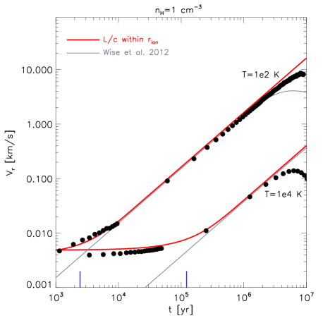
Figure 3: Velocity as a function of time for gas with the same initial density $n_{\rm H}=1\,\rm cm^{-3}$ but different fixed temperatures: $T=10^{2}\,\rm K$ (top) and $T=10^{4}\,\rm K$ (bottom). The velocities acquired via radiation pressure become larger the colder the gas is (see text for more details). Results measured in the simulations (black dots) agree well with analytical estimations from Eq. (9) (red curve) at both temperatures. Gray lines correspond to the predictions in the case of an optically thick shell (Wise et al. 2012), which coincides with our analytic estimate for $t>t_{\rm rec}$. At later times, mass entrainment will slow down the gas, an effect not considered in Eq. (9) but which can be seen in the thick shell formulation as a turn over of the gray curve at $t\sim 4\times 10^{6}\,\rm yr$. The true behaviour of the gas at these late stages will lie somewhere between our analytic estimate and the optically thick shell formulation.

Figure 1 suggests that the momentum input by radiation is distributed more or less uniformily within the ionized region. For a constant density $n_{\rm H}$, we can then compute the expected velocity of the gas analytically:

$$V_{r}(t)=Lt/(c\;m_{\rm ion}),$$ (9)

where $V_{r}$ and $m_{\rm ion}$ are the radial velocity and mass of the gas within the ionized region at time $t$ and $L$ the luminosity of the source.

Fig. 2 shows excellent agreement between this simple estimate and the results of the radiative transfer code for a variety of gas densities. Interestingly, $V_{r}$ shows two regimes established around the recombination time: an early phase where the gas velocity remains approximately constant (as the ionizing front carves its way into the neutral gas) and a later regime for $t>t_{\rm rec}$ where the velocity of the gas increases linearly with time. This behaviour can be understood in terms of the size of the ionized sphere. When $r_{\rm ion}<r_{s}$, the mass in which the momentum is deposited increases with time while the ionization front runs to its final equilibrium value $r_{\rm ion}=r_{s}$. Once the equilibrium between ionizations and recombinations is reached at $t\sim t_{\rm rec}$, $m_{\rm ion}$ remains stationary and we expect a linear dependence of $V_{r}$ with time, as in Eq. (9).

The different panels in Fig. 2 indicate that the gas velocity becomes larger with increasing gas density. This is because for high $n_{\rm H}$, the same momentum is being distributed within a smaller region containing less mass than in a more diffuse media; $r_{\rm ion}^{3}\propto n_{\rm H}^{-2}$ and $m_{\rm ion}\propto n_{\rm H}^{-1}$. Radiation pressure is therefore most relevant – in terms of achieving large velocities – in high density gas.

Temperature also determines the size of the ionized region and can therefore have an impact on $V_{r}$. At fixed density and luminosity, low temperature gas recombines more efficiently, with a recombination coefficient $\alpha_{\rm B}(T)\propto(T/10^{4})^{-0.85}\rm cm^{3}\,s^{-1}$ (Dopita & Sutherland, 2003). Figure 3 shows that by reducing the temperature from $T=10^{4}\,\rm K$ to $10^{2}\,\rm K$, the radial velocity of the gas increased by a factor $\sim 50$, corresponding to the different $\alpha_{\rm B}$ in each case. As before, we find very good agreement between the results of the numerical simulations with radiative transfer (black dots) and predictions from the analytical estimate in Eq. (9) (thick solid red lines). The simple assumptions that go into Eq. (9) seem to overestimate the gas velocity at early times ($t\ll t_{\rm rec}$), but the discrepancy is less than $30\%$.

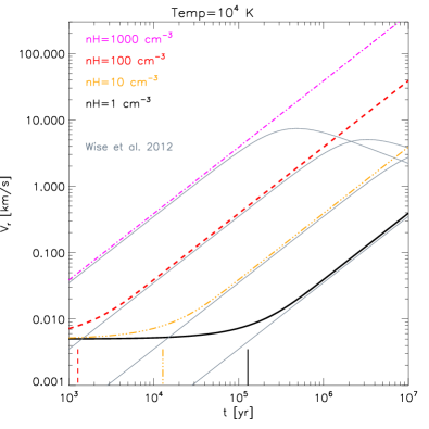
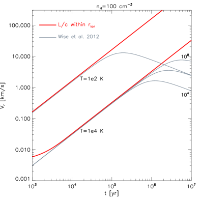
Figure 4: Analytical predictions for gas velocity due to radiation pressure. The left panel shows that $V_{r}$ increases linearly with gas density; coloured lines correspond to Eq. (9) and gray ones to the optically thick shell approximation from Eq. (3). The right panel explores, at fixed $n_{\rm H}=100\,\rm cm^{-3}$, the effects of gas temperature and luminosity of the source: $V_{r}$ grows as $\propto(T/10^{4})^{-0.85}$ with decreasing gas temperature but is almost independent of the luminosity of the source (lower curves correspond to $L=10^{4}$, $10^{6}$, and $10^{8}\,\rm L_{\odot}$). This is because more powerful sources also have larger Strömgren spheres, such that their momentum is distributed onto larger masses. These effects cancel out in Eq. (9), producing a single curve irrespective of $L$ (red curves). However, the luminosity of the source will determine – towards the end of the lifetime of stars – when mass entrainment takes over in the optically-thick shell formalism, as shown by the three gray curves in the $T=10^{4}\,\rm K$ set.

Despite the fact that the systems behave differently than in the simplistic optically-thick shell scenario, Fig. 3 shows that the predicted velocities are similar in the two cases. Gray lines correspond to the analytic estimate of the gas velocity for an optically-thick shell of gas presented in Eq. (3) (taken from Eq. 5 in Wise et al. 2012). Although it does not match the initial phase of expansion of the ionized region, both expressions agree well in the region of linear growth. At later times, mass removed from the inner regions starts to accumulate, slowing down the gas (see the turn over in the gray curve at $T\sim 5\times 10^{6}\,\rm yr$ in the $T=100\,\rm K$ case). This effect is not taken into account in Eq. (9), which continues to increase linearly. The results of the radiative transfer simulation in the $T=100\,\rm K$ run suggest that the true velocity of the gas should fall somewhere in between both estimates.

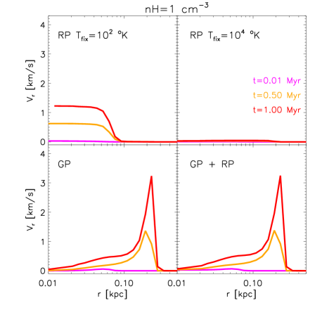
Figure 5: Radial velocity of gas as a function of radius obtained in a uniform box with density $n_{\rm H}=1\,\rm cm^{-3}$ for different configurations: radiation pressure only with fixed temperature $T_{\rm fix}=10^{2}\,\rm K$ (upper left) and $T_{\rm fix}=10^{4}\,\rm K$ (upper right), photoionization only (bottom left) and combined effects of photoionization and radiation pressure (bottom right). Simulations in the bottom row where initialized with $T=10^{2}\,\rm K$, and the temperature evolution was followed self-consistently to account for heating and cooling processes. Colours correspond to three different times as labeled. The similarity between the left and right panels in the bottom row suggests that the effect of radiation pressure is sub-dominant once photoionization is taken into account.

The good agreement between the radiative transfer calculations and the analytic estimates from Eq. (3) and (9) allows us to gain some intuition about the impact of stellar radiation on surrounding gas. Figure 4 summarizes the effect of varying the three primary variables involved in the radiation pressure problem:

• Gas density (left panel): as explained above, $V_{r}$ increases linearly with density at fixed temperature and luminosity. Notice, however, that for the typical lifetime of massive stars, $1-5\times 10^{6}\,\rm yr$, the expected velocities due to radiation pressure in gas of temperature $T=10^{4}\,\rm K$ are small. Even for densities as high as $n_{\rm H}=100\,\rm cm^{-3}$, the characteristic density of molecular clouds, they only reach $V_{r}\sim 5-20\,{\rm km\,s^{-1}}$. This by itself is too low to drive galactic winds, but it is large enough to unbind gas clouds in the ISM.

• Gas temperature (right panel): the gas velocity increases with lower temperatures, because the size (and therefore, the mass) of the Strömgren sphere also decreases for colder gas. Notice, however, that the mono-chromatic set-up of our experiments does not yield a fully realistic temperature evolution of the ionized region.

• Luminosity of the source (right panel): $V_{r}$ is only weekly dependent on the luminosity of the source. Larger luminosities translate into larger Strömgren spheres and therefore a larger $m_{\rm ion}$, in such a way that $V_{r}$ stays constant. The right panel of Fig. 4 shows the velocity of the gas at three different luminosities, $10^{4}$, $10^{6}$, and $10^{8}\,\rm L_{\odot}$, for the $T=10^{4}\,\rm K$ case. The three curves perfectly overlap for Eq. (9) (red line), and only seem to differ at late times if we consider the optically-thick shell scenario (see three gray curves). This means that for a large fraction of the lifetime of the HII region, the total momentum input per affected gas mass is independent of luminosity. However, after $\sim 1\,{\rm Myr}$ powerful sources might give rise to larger velocities, depending on the detailed behaviour of mass entrainment and the available time before a supernova explosion.

3.2 Radiation pressure combined with photoionization effects

For most cases of astrophysical interest, the sources of radiation in the ISM will be massive stars with spectral emission well approximated by a black-body spectrum of effective temperature $T_{\rm BB}\sim 10^{5}\,\rm K$ (i.e. not monochromatic as assumed above). In this case, photons will not only ionize but also heat up the gas to a temperature $T\geq 10^{4}\,\rm K$. If the medium was originally at a lower temperature, this hotter gas within the ionized bubble will create a pressure gradient outwards, pushing the gas radially away from the source. In this case, it is the energy as well as the momentum of the radiation that will have an impact on the dynamics of the gas. The role played by the radiation pressure should therefore be analyzed in tandem with the effects of photoionization.

In Fig. 5, we compare the effects of photoionization and radiation pressure in detail. We show the gas velocities as a function of radius in our radiative transfer simulations where we have considered different mechanisms: radiation pressure alone at fixed temperatures $T_{\rm fix}=10^{2}\,\rm K$ (top left) and $T_{\rm fix}=10^{4}\,\rm K$ (top right), photoionization alone with an initial temperature $T=10^{2}\,\rm K$ (bottom left) and photoionization plus radiation pressure, also with initial temperature $T=10^{2}\,\rm K$ (bottom right). Colored lines show different times during the evolution, $t=0.01$, $0.5$ and $1\,\rm Myr$. All boxes have an initial constant density $n_{\rm H}=1\;\rm cm^{-3}$. Notice that in the upper row we use a monochromatic source (i.e. temperature is approximately fixed) whereas the bottom row uses a black-body spectrum with temperature $T_{\rm BB}=10^{5}\,\rm K$ and follows the heating and cooling of the gas self-consistently as described in Sec. 2. We have checked that the results in the top panels do not change if we use instead a black-body source and switch-off the heating in the code manually. In all cases, the luminosity of the source is $L=10^{6}\,\rm L_{\odot}$.

The upper panels in Fig. 5 confirm that radiation pressure, when acting alone, is more efficient in cold gas. For example, after a million years, $V_{r}$ reaches $\sim 1\,\rm km\,s^{-1}$ in the $T_{\rm fix}=10^{2}\,\rm K$ run compared to negligible values for $T_{\rm fix}=10^{4}\,\rm K$ (see also Fig. 3). However, tracking the temperature evolution in a more realistic way shows that photoionization alone can also yield relevant velocities; reaching in this example $V_{r}\sim 3\,\rm km\,s^{-1}$ in the same time-span (bottom left panel) .

Inspection of the left column of Fig. 5 shows that photoionization and radiation pressure induce a different velocity profile; radiation pressure affects only the inner regions within the Strömgren sphere whereas photoionization induces velocities that peak slightly beyond $r_{s}$. It is therefore interesting to look at the joint action of both mechanisms, shown in the bottom right panel. The similarity between the runs labelled “GP” (gas pressure) and “GP + RP” (gas pressure + radiation pressure) in the bottom row suggests that radiation pressure does not play an important role in the dynamics of the gas for this experiment once photoionization is taken into account.

This is better seen in the left panel of Fig. 6, where we overlap the run with photoionization alone (red curve) and photoionization plus radiation pressure (blue) at a much later time $t\sim 10\,\rm Myr$, corresponding to approximately $\sim 150\,t_{\rm rec}$, where $t_{\rm rec}$ is the recombination time of the ionized gas ($\sim 1.2\times 10^{5}\,\rm yr$). The difference between both curves is negligible, as shown by the differential curve in the bottom inset. A similar conclusion is reached for much denser gas, $n_{\rm H}=100\,\rm cm^{-3}$ (right panel), where the radiation pressure adds only $\sim 0.5\,\rm km\,s^{-1}$ in regions of the gas moving at $V_{r}\sim 9\,\rm km\,s^{-1}$ due to photoionization alone. A closer comparison of the simulations shows that, as soon as ionization starts, it quickly raises the gas temperature to $T\sim 10^{4}\,\rm K$, pushing the system to the high temperature regime where radiation pressure is less effective. Therefore, even in high density, initially low temperature gas, radiation pressure has only a small effect on the dynamics of the gas. Its influence is mostly overwhelmed by pressure gradients originating from photoionization.

An important caveat from Fig. 6 lies in the time at which we examine the system. For a density $n_{\rm H}=100\,\rm cm^{-3}$, $t\sim 250\,t_{\rm rec}$ corresponds to an absolute time of $\sim 0.3\times 10^{6}\,\rm Myr$, which falls short by a few million years compared with the expected life time of massive stars. Unfortunately, we had to stop this simulation because the shell of material removed from the inner regions reached the border of the box at $L_{\rm box}=30\,\rm pc$ so that we could no longer track the evolution of the bubble. However, we can confidently place upper limits on the effect of radiation pressure by using the analytic estimate from Eq. (9). The bottom inset in the right panel of Fig.  6 shows that the boost in the gas velocity due to radiation pressure is $V_{r}\sim 0.5\,\rm km\,s^{-1}$, approximately the velocity predicted for a gas of the same density and temperature $T=10^{4}\,\rm K$ if we consider radiation pressure only (see Fig. 4). Using this analytic calculation, the dashed red curve in Fig. 4 indicates that radiation pressure will push the gas with speeds no larger than $\sim 10\,\rm km\,s^{-1}$ over a period of a few million years. This is comparable to the velocity caused by photoionization in a tenth of that time. Moreover, this calculation is an optimistic upper limit, since the early action of photoionization will lower the density of the inner regions of the gas, thereby reducing the impact of radiation pressure.

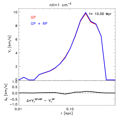
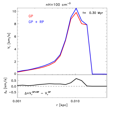
Figure 6: Radial velocity profiles of the gas in the photoionization only (red) and photoionization plus radiation pressure (blue) runs after $\sim 150\,t_{\rm rec}$. Both experiments are initialized with constant density, $n_{\rm H}=1\,\rm cm^{-3}$ (left) and $n_{\rm H}=100\,\rm cm^{-3}$ (right), $T=100\,\rm K$ and the temperature is allowed to vary following heating/cooling mechanisms. The difference between the red and blue curves is strikingly small, supporting a scenario where the dynamics of the gas is completely dominated by photoionization (see text for more details). The bottom insets show the velocity difference between both curves, which corresponds to an increase $\Delta V_{r}<0.5\,\rm km\,s^{-1}$ for $n_{\rm H}=100\,\rm cm^{-3}$, and even smaller for $n_{\rm H}=1\,\rm cm^{-3}$.

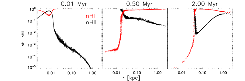
Figure 7: Ionization profiles for the isothermal gas cloud C2 ($\sigma=3\,\rm km\,s^{-1}$) and a black-body central ionizing source with $L=10^{6}\,L_{\odot}$ and $T_{\rm BB}=10^{5}\,\rm K$. The profiles are more complex than in the constant density case (e.g. see Fig. 1). As before, the ionization front moves outwards with time and is located at $\sim 4\,\rm pc$ after $2\,\rm Myr$. We refer to this case as an “optically thick” cloud to distinguish it from one in which the ionization front has reached the border of the box.

We conclude that for stellar sources surrounded by constant density gas, photoionization will typically dominate the dynamics of the gas over direct radiation pressure, unless the density is very high, $n_{\rm H}\geq 1000\,\rm cm^{-3}$. Such high densities are not common on the scale of whole molecular clouds, but could be reached in small regions close to their cores. We investigate this possibility below.

Table 2: Summary of properties of our isothermal-profile gas clouds. We list their velocity dispersion $\sigma_{\rm cl}$, temperature $T$, central mean density $\left<n_{\rm H}\right>$ computed within $5\,\rm pc$, the mass enclosed within $10$ and $100\,\rm pc$, the luminosity of the central source $L$, the total end radius of the clouds $R_{\rm tot}$, and the number of cells used in the initial conditions $N$. In all the runs, the gravitational softening is $\epsilon=2\,\rm pc$.

Label	$\sigma$	$T$	$<n_{H}>(r<5\;\rm pc)$	$M(r<10\;\rm pc)$	$M(r<100\;\rm pc)$	L	$R_{\rm tot}$	N
	[$\rm km\,s^{-1}$]	$[\rm K]$	$[\rm cm^{-3}]$	$[10^{4}\,\rm M_{\odot}]$	$[10^{4}\,\rm M_{\odot}]$	$[\rm L_{\odot}]$	$[\rm kpc]$
Cloud 1 (C1)	1	60.57	85.4	0.18	2.27	$10^{4}$	1	$128^{3}$
Cloud 2 (C2)	3	545.17	810.5	1.51	20.5	$10^{6}$	3	$128^{3}$
Cloud 3 (C3)	6	2180.70	3555.6	6.5	81.0	$10^{7}$	6	$256^{3}$

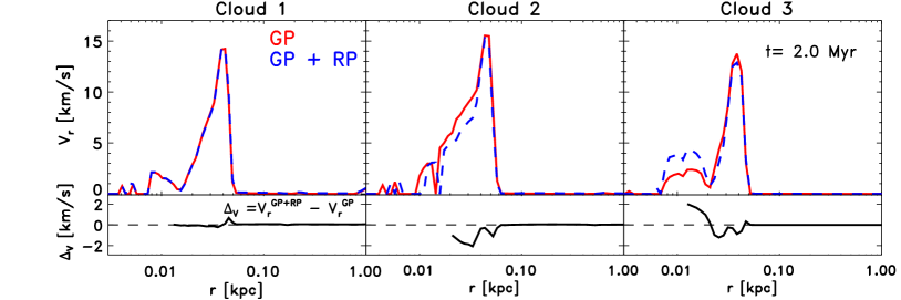
Figure 8: Radial velocity of the gas after $t=2\,\rm Myr$ for isothermal-profile clouds with (blue, GP+RP) and without (red, GP) radiation pressure. Lower insets show the difference between both curves $\Delta_{V}=V_{r}^{\rm GP+RP}-V_{r}^{\rm GP}$, which is very small.

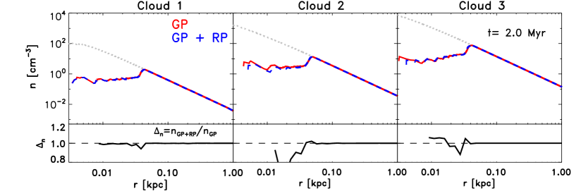
Figure 9: Final density profile for isothermal-profile gas clouds run with (blue, GP+RP) and without (red, GP) radiation pressure. The results correspond to $t=2\,\rm Myr$. The impact of radiation pressure is smaller than $\sim 20\%$, as shown by the ratio between both profiles $\Delta_{n}=n_{\rm H}^{\rm GP+RP}/n_{\rm H}^{\rm GP}$ in the bottom inset panels.

4 Radiation pressure in gas clouds with isothermal profiles

In this Section we relax our assumption of constant density gas and explore the effects of radiation pressure and photoionization in isothermal density profiles, $\rho\propto r^{-2}$. This provides a better description of the gaseous clouds where stars are born (although the exact structure of molecular clouds can show large variations, e.g. Heyer et al., 2009). A detailed model of radiation pressure in realistic molecular clouds is out of the scope of this paper (it would require to include sources of turbulence, resolve individual star formation, model the effects of metallicity, etc.). Instead, we aim to highlight, using a series of idealized experiments, the role played by the density distribution of the gas on the relative interplay between radiation and photoionization pressure.

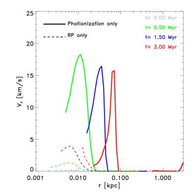
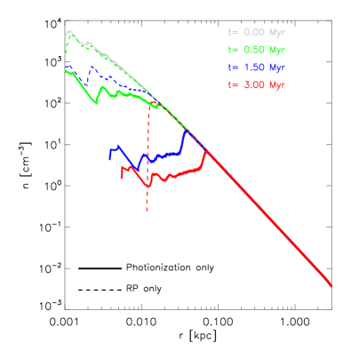
Figure 10: Further diagnostics of the isolated effects of radiation pressure compared to photoionization. We show the velocity (left) and the density profile (right) of the C2 cloud at different times (coloured lines) for runs where only photoionization (solid) or only radiation pressure (dashed) are taken into account. Radiation pressure has the ability to modify the velocity and mass distribution of the cloud, emptying the inner $\sim 10\,\rm pc$ of the cloud in $\sim 3\,\rm Myr$. But the time needed for this is longer than the time required by photoionization to start affecting the medium. The left panel shows that at any given time (same colours), photoionization has a larger velocity than radiation pressure. Thus, when both effects are considered, photoionization sets in quicker, heating and pushing the gas with the result of lowering the central densities on a shorter timescale. This in turn diminishes the impact of the radiation pressure even further. This explains the small differences between red and blue curves in Fig. 8 and 9.

We consider three gas clouds C1-C3 with the properties listed in Table 2. Each cloud was set up in hydrostatic equilibrium, which defines a relation between total mass, radius, velocity dispersion and temperature by specifying only one of the four variables (Binney & Tremaine, 2008). Table 2 includes the mass contained within $10$, and $100\,\rm pc$ (columns 5 and 6) which may help to relate them to known objects in the local Universe. Object C1 is an example of a fluffy low mass cloud hosting a late B-type star, a good representative of the $M\sim 10^{3}\,\rm M_{\odot}$ objects populating the low mass end of the compilation of molecular clouds by Heyer et al. (2009). C2 and C3 are more massive examples hosting a source with a luminosity of a couple of OB stars. They are consistent with clouds of mass $\sim 5\times 10^{4}$, $5\times 10^{5}\,\rm M_{\odot}$ and sizes of $20$, $50\,\rm pc$ respectively (Heyer et al. 2008, see also Fig. 3 in Dale et al. 2012 for a graphical display of the data).

The initial conditions of each cloud were evolved in isolation for $1\,\rm Gyr$ to verify their dynamic stability. No structural change was observed. We added a massless central source of ionizing radiation with a given luminosity (see Table 2) and a black-body spectrum with temperature $T_{\rm BB}=10^{5}\,\rm K$. The luminosities were chosen such that all clouds will remain optically thick for a few million years. We performed radiative transfer simulations with our code, following the heating and cooling of the gas, the hydrodynamics and the gravity forces.

The ionization profiles in our clouds are now more complex (see Fig. 7) compared to the simple case shown in Fig. 1. This is not only the result of the declining density profile, but also of the spectral shape of the ionizing source. The high energy photons from the $10^{5}\,\rm K$ black-body spectrum can penetrate deeper into the cloud and ionize distant regions before the bulk of the $E_{0}\sim 13.6\,\rm eV$ photons fully ionize the interior of the cloud. It is still possible to define an ionization radius as the smallest radius where the neutral fraction is larger than $0.5$. As mentioned before, we only focus on clouds where $r_{\rm ion}$ is smaller than the final radius of the cloud – the optically thick regime – and defer an analysis of fully ionized clouds to future work.

Fig. 8 shows a comparison between the velocity as a function of distance in our clouds considering photoionization alone (red) and photoionization plus radiation pressure (blue). We show the results after 2 Myr of evolution, the time at which the input from radiation pressure is maximum (Krumholz & Matzner, 2009). As in the previous section, we again find that adding radiation pressure to our calculations does not change the gas velocity by a significant amount. Fig. 8 shows that the velocity in the run were both radiation pressure and gas pressure effects are considered is either equal or even smaller than in a run with thermal pressure alone. The lower velocities are caused by an enhanced mass removal from the center of the clouds when radiation pressure is included, but this effect is small. Fig. 9 shows that the gas density in the centers can be lower by up to $\sim 20\%$ in the run with radiation pressure compared to considering only photoionization. This is also true for C3, our cloud with the highest mass and most powerful source, i.e., our most optimistic candidate for radiation pressure effects. C1, on the other hand, shows no difference between both runs. In all cases, photoionization alone generates velocities $V_{r}\sim 15\,\rm km\,s^{-1}$, flattening the inner density profile of the clouds and dominating the overall evolution in time.

The relatively small impact of radiation pressure in Fig. 8 and 9 is perhaps surprising: analytic arguments and the results of the radiative transfer calculation from the previous Section have shown that radiation pressure can potentially drive significant velocities, especially for high densities. Why then do our simulated clouds show such a small effect due to radiation pressure? To answer this question one has to consider the characteristic timings associated with each process, photoionization and radiation pressure.

To investigate this in more detail, we run the C2 cloud including only photoionization or only radiation pressure (no temperature evolution), leaving everything else unchanged. The results of this exercise are shown in Fig. 10. Photoionization (solid curves) proceeds relatively quickly, raising the velocity of the gas above $V_{r}\sim 15\,\rm km\,s^{-1}$ in less than a million years. The peak velocity moves outwards with time, decreasing slightly in magnitude. In contrast, radiation pressure (dashed curves) requires longer times to deposit the momentum in the media, exciting a maximum velocity of only $V_{r}\sim 5\,\rm km\,s^{-1}$ after 2 or $3\,\rm Myr$.

A similar effect is seen in the density profiles (right panel of Fig. 10). Radiation pressure (dashed curves) eventually pushes all the gas within $r=10\,\rm pc$, emptying the core of the cloud. But it does it slowly, with only minor modifications in the profile for the first $\sim 1.5\,\rm Myr$ of evolution. Instead, photoionization starts emptying the inner regions considerably faster, with less than $5\times 10^{5}\,\rm yr$ required to produce appreciable changes in the inner regions of the cloud (see solid green line). After $3\,\rm Myr$, photoionization alone has lowered the density of the core by more than three orders of magnitudes.

This time delay in the build up of the effects of radiation pressure with respect to photoionization makes it less relevant than expected. Radiation pressure needs a comparatively long time period to deposit the momentum in the gas. The photoionization timescales are shorter, yielding an early removal of gas from the cloud centre. This limits the effects of radiation pressure even further, which require large densities to maximize the momentum input. Radiation pressure in the single scattering limit is therefore sub-dominant compared with photoionization effects in the gas for both mass distributions explored here, a constant density medium and a declining $r^{-2}$ density profiles.

5 Discussion and conclusions

It is interesting to contrast the results of our radiative transfer calculations with some analytic predictions. Krumholz & Matzner (2009) have shown that the pressures due to radiation and due to photoionization have different radial dependences, meaning that there is a characteristic radius $r_{\rm ch}$ within which radiation pressure is expected to dominate while further out gas pressure takes over. This characteristic radius is typically small for the average molecular clouds in the Milky Way, where photoionization might be the dominant mechanism for cloud destruction (see Walch et al. 2012). However, for the most dense clouds hosting luminous sources, $r_{\rm ch}$ can reach a few hundred parsecs, so that radiation pressure might be able to completely unbind them.

We have used equations 6 and 8 from Krumholz et al. to estimate $r_{\rm ch}$ for the clouds studied in Sec. 4. For C1 and C2, we obtain values smaller than our resolved region ($r_{\rm ch}=1\times 10^{-2}$ and $1.5\,\rm pc$, respectively), thus the dominance of gas pressure found in our simulations for $r>5\,\rm pc$ would be expected in this scenario. But our most massive cloud, C3, has $r_{\rm ch}=20\,\rm pc$, a region well resolved in our analysis. Nevertheless, for C3 we also find a negligible impact of radiation pressure on the central density of the cloud after $t=2\,\rm Myr$. This is not necessarily a disagreement, as the analytical estimates by Krumholz et al. explore the effect of radiation pressure on the position and velocity of expansion of the ionization front, and not on the gas in the clouds, as explored here. The I-front velocity can differ substantially from the actual bulk velocity induced in the gas (for example, compare Fig. 12 and 18 in Iliev et al. 2009). In our results, radiation pressure does not dominate the gas dynamics and hence the structure of the cloud at any radius.

In general, we find that radiation pressure is a relatively slow and inefficient way of coupling radiation to the surrounding gas. This can be understood with a simple example. Let us consider the case of a hydrogen atom that absorbs a single 13.6 eV photon. The momentum deposited in that atom will push it with velocity $V_{r}\sim 5.6\,\rm m\,s^{-1}$, requiring more than thousand ionizations from the same direction for a single atom to achieve a modest velocity of $V_{r}\sim 10\,\rm km\,s^{-1}$. The core of the problem is that, once the atom is ionized, it takes some time to recombine and be available to receive the next velocity kick. That is why radiation pressure is slow compared to photoionization, which only requires a short time for the thermalization of the energy above $E=13.6\,\rm eV$ of a single ionization event. The inefficiency of direct radiation pressure has been suggested before (Mathews, 1969; Spitzer, 1978; Arthur et al., 2004; Krumholz & Matzner, 2009; Kim et al., 2013), but has not been confirmed rigorously in simple configurations with appropriate radiative transfer calculations.

Encouragingly, our findings are in good agreement with recent observational results of HII regions, where gas pressure seems to dominate over radiation (Lopez et al., 2013), as well as with numerical modelling of clouds (Dale et al., 2013). The results of our experiments have direct consequences for the sub-grid modelling of radiation pressure at the scale of galaxy simulations. Arguably the most important lesson is that the “mass loading” (i.e. the mass in which the photon momentum is deposited) is not a free parameter but is determined by the size of the ionized region. This agrees with the recent work by Renaud et al. (2013), but disagrees with many previous models where the mass loading was chosen in an ad-hoc fashion (Oppenheimer & Davé, 2006; Agertz et al., 2013; Aumer et al., 2013; Ceverino et al., 2013). This can have a sizable impact on the effectiveness associated with radiation pressure feedback in these numerical codes, since by choosing a sufficiently small mass loading, the velocity given to the gas can be increased almost arbitrarily (within the constraints of the total momentum input from the ionizing source).

Under general conditions in the ISM, photoionization due to massive stars has an impact on the dynamics of the gas that is comparable to and typically more important than that of direct radiation pressure. From the point of view of numerical modelling, the “early feedback” implementation by Stinson et al. (2013) seems to be a step in the right direction, in the sense that it actually uses thermal pressure rather than radiation pressure. A problematic point is however that there is still lots of freedom when choosing the total energy budget released by the young stars and how this is distributed from the stars to the neighboring SPH particles. The effects of photoionization are also starting to be included in semi-analytical models with promising results (e.g. Lagos et al., 2013).

Fig. 4 shows that radiation pressure might be able to generate competitive velocities $V_{r}\geq 50\,\rm km\,s^{-1}$ only for very high density gas, $n_{\rm H}\geq 1000\,\rm cm^{-3}$, although this is uncertain up to the exact slow-down effect due to the mass accumulation (a shell-like approximation predicts that such velocities will never be reached). But even neglecting the mass entrainment, such high densities – necessary to get very short recombination times – are uncommon, occurring only in the most massive molecular clouds in the Milky Way, or are restricted to particular environments such as vigorous starbursting galaxies or gas-rich proto-galaxies in the early Universe. Radiation-pressure driven winds are hence unlikely to be important for the general locus of galaxies unless we assume large boosting factors due to radiation trapping in dust grains.

An assessment of the potential effects of dust on our study is not straightforward as the presence of dust makes the effective Strömgren radius smaller than the corresponding dust-free case (see chapter 5 Spitzer 1978). However, we can place some upper limits based on the predictions from Fig. 4, which tend to be conservative as they ignore the effects of photoionization taking place earlier than the radiation pressure. At the average density of molecular clouds, $n_{\rm H}=100\,\rm cm^{-3}$, we need to boost the velocities by a factor $\tau\sim 30$ to achieve $V_{r}\sim 400-600\,\rm km\,s^{-1}$ comparable to the escape velocity in $L_{*}$ galaxies. This would lie at the upper end of conceivable boost factors according to current estimates (Hopkins et al., 2011), but there have been some recent discussions about the plausible upper end (Krumholz & Thompson, 2012).

We recall that we have simulated radiation pressure under highly idealized conditions with the aim to explore in detail its interplay with photoionization and their combined dynamical imprint on the gas. Several caveats are unavoidable when taking such an approach. In particular, our results deal with spherically symmetric systems and consider only hydrogen ionization. We also neglect any effect due to the complicated small-scale structure of the ISM, which we approximate as a well mixed, isothermal medium. Obvious gaps in our analysis concern the presence of “champaign flows” (e.g. Yorke et al., 1983) or the acceleration of confined cold clouds within a hot medium created by ionization. But in turn, the advantage in using idealized models lies in providing a clean understanding of the interaction between radiation and the dynamics of the gas under conditions that are typical in galaxies. This helps to narrow down the regime in which an inclusion of the effects of radiation pressure is required. The results presented here might also be useful for developing more realistic sub-grid models for simulations of galaxy formation.

Appendix A Standard Radiative Transfer Tests

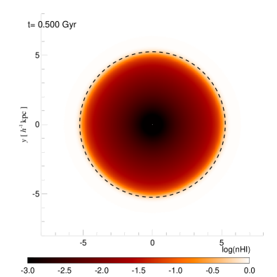
Figure 11: Left: Eigenvectors of the Eddington Tensor for a single central source in Test 1. Right: Map of neutral gas fraction for a central slab in a $64^{3}$ cells run after $t=500\,\rm Myr$. The Strömgren radius is indicated with a black dashed line.

In this section we report the performance of the radiative transfer module for the set of tests proposed in the radiative transfer code comparison work by Iliev et al. (2006), augmented with the dynamical “Test 5” in Iliev et al. (2009). The initial set-ups are the ones used previously in the gadget version of the module presented in Petkova & Springel (2009). Refinement/de-refinement of cells is not required in these tests as they deal mostly with static and equal-density gas configurations, except for the last test. Although the code has the capability to work with a mixture of hydrogen and helium gas, in the interest of simplifying a comparison with previous work, the gas is assumed to be composed of hydrogen only.

A.1 Test 1: Pure hydrogen isothermal HII region expansion

We study the ionization profiles in a constant density box with $L_{\rm box}=16\,\rm kpc$ on a side. We use a central source emitting $5\times 10^{48}\,\rm photons\,s^{-1}$. The temperature is fixed at $\rm T=10^{4}\,\rm K$, and the gas density is $n_{\rm H}=10^{-3}\,\rm cm^{-3}$. The radiation is mono-chromatic with energy $E_{0}=13.6\,\rm eV$. For the numbers above, the recombination time is $t_{\rm rec}=125\,{\rm Myr}$ and the Strömgren radius is $r_{s}=5.38\,{\rm kpc}$.

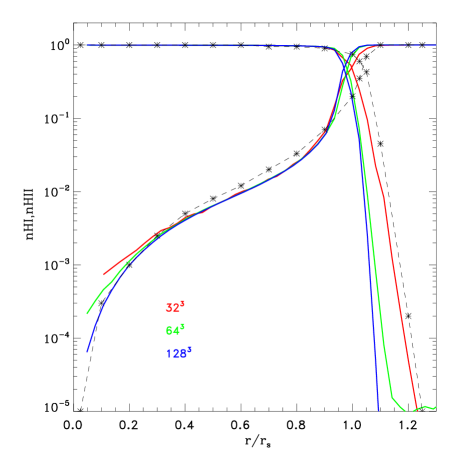
Figure 12: Neutral fraction profile for a single source in a box with $32^{3}$, $64^{3}$ and $128^{3}$ cells (Test 1). Dashed line/asterisks shows the theoretical solution taken from PS09. Overall, we find excellent convergence of results with the number of cells.

We show a projection of the (dominant) eigenvectors of the Eddington tensor in a thin slab of the box (right panel of Fig. 11). The tensor determines the direction of the radiation transport, which is radially away from the source for our specific case. The right panel in Fig. 11 shows an intensity map of the neutral gas fraction after $500\,{\rm Myr}$ of evolution. The black dashed line indicates, as expected, that the Strömgren radius coincides with the radius beyond which the gas remains neutral. We use $64^{3}$ cells for this experiment and test the numerical convergence with the number of cells below.

Fig. 12 shows that the neutral/ionized gas profiles are in good agreement with the theoretical predictions (dashed black line connecting asterisks). We find that the flux-limiter determines to a certain extent the shape of these profiles and use this fact to calibrate the flux-limiter formula in our code. We settled for the Levermore & Pomraning (1981) flux-limiter (see Eq. 5), which in our case matches the analytical solutions better than the one used previously in PS09. Different colours in Fig. 12 show that the results converge well with the number of cells ($32^{3}$ in red, $64^{3}$ in green and $128^{3}$ in blue).

We explore the effects of different time-stepping in Fig. 13. We show the time evolution of the ionization radius for this test with fixed individual (global) time-steps $\Delta t=50$, $5$ and $0.5\,\rm Myr$. The black dashed line shows the result from the analytic formula in Eq. (8). The agreement improves for runs with small time-steps, which are able to better resolve the early evolution of the front. For instance, for $\Delta t=5\,\rm Myr$, the simulated and analytical results agree well only after $t\sim 3\,t_{\rm rec}$; instead, a simulation with 10 times smaller time-steps describes the whole time evolution of the ionization front accurately.

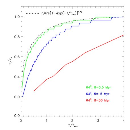
Figure 13: Effect of time-step size on the I-front propagation. We use a $64^{3}$ grid. A time-step shorter than $0.5\,\rm Myr$ nicely reproduces the expected theoretical results (dashed black curve).

Finally, we also explored a double-source set up as suggested by Gnedin & Abel (2001) and PS09. This test has the same parameters for gas and source as before, but we employ two sources (instead of one) separated by $8\,\rm kpc$. Their Strömgren spheres do overlap and we end up with a shared, elongated ionized bubble after $500\,\rm Myr$, as shown in the right panel of Fig. 14. Our results agree well with those in PS09.

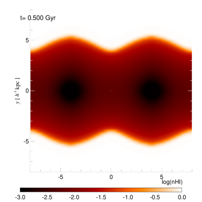
Figure 14: Same as Fig. 11 but for two nearby sources. We use $64^{3}$ cells.

A.2 Test 2: HII region expansion: the temperature field

This test consists of a static uniform density field within a box of side-length $16$ kpc, in which we place a central source emitting $5\times 10^{48}\,\rm photons\,s^{-1}$ with a black-body spectrum of temperature $T=10^{5}\,\rm K$. Initially, the gas is set to density and temperature equal to $n_{\rm H}=10^{-3}\,\rm cm^{-3}$ and $T=10^{2}\,\rm K$, respectively, with the latter being allowed to change according to the heating and cooling mechanisms described in Sec 2.

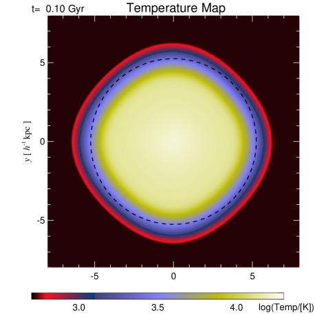
Figure 15: Temperature map corresponding to Test 2 after $t=100\,\rm Myr$. For guidance, we show the Strömgren radius from Test 1 with a dashed black line.

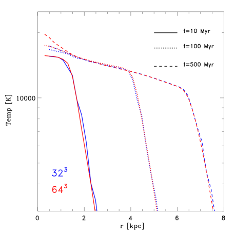
Figure 16: Spherically averaged temperature profiles in the HII region from Test 2 at three different times. We obtain good convergence of the results when varying the number of cells ($32^{3}$ in blue, $64^{3}$ in red).

Fig. 15 shows a temperature map in a central slice through the simulated box at $t=0.1\,\rm Myr$. Unlike in the previous test, a set-up with varying temperature does not have an analytical solution for the size of the Strömgren sphere. For reference we also show the Strömgren radius corresponding to Test 1, that has the same conditions but fixed $T=10^{4}\,\rm K$ (dashed black line). Photoionization proceeds slightly beyond this estimate, probably due to the presence of high-energy photons that are able to penetrate deeper into the neutral gas.

Fig. 16 shows in more detail the temperature profiles at three different times $t=10$, $100$ and $500\,\rm Myr$, and for two different resolutions corresponding to $32^{3}$ and $64^{3}$ cells. The results show excellent numerical convergence and their behaviour with time and radius agrees well with those reported in PS09 and Iliev et al. (2006). The same is true for the neutral/ionized gas profiles shown in Fig. 17. Here the action of more energetic photons, which smooth out the transition between ionized and neutral region compared to a mono-chromatic source like in Test 1, can be clearly appreciated.

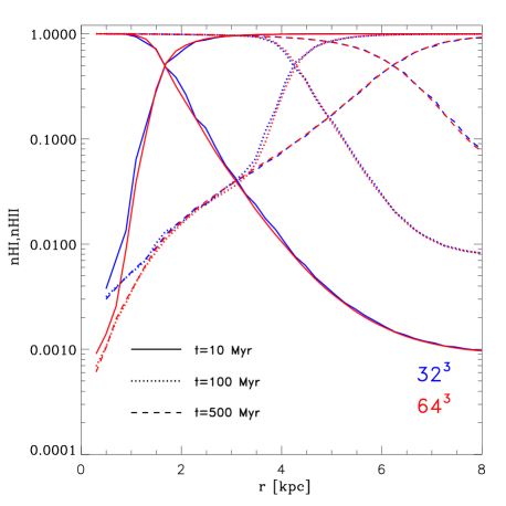
Figure 17: Same as Fig. 16, but for the neutral/ionized gas profile.

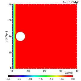
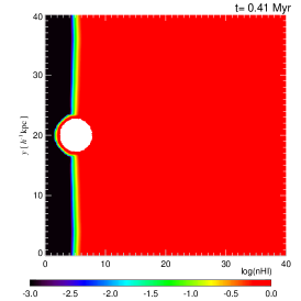
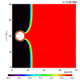
Figure 18: Shadow test: Ionized fraction in a slide through the middle of the box at three different times (Test 3). The evolution is as expected, but notice that the OTVET approximation fails to cast a sharp shadow after the I-front has advanced beyond the center of the clump. This extra diffusion is expected and a well known issue of this method.

A.3 Test 3: I-front trapping in a dense clump and the formation of a shadow

This set-up follows exactly the test presented in PS09, which in turn is inspired by Test 3 in Iliev et al. (2006). It consists of a box with length 40 kpc on a side filled with gas at density $n_{\rm H}=10^{-3}\,\rm cm^{-3}$ that contains a cylinder $10^{5}$ times denser. Radiation comes from a plane of (512) stars located in the $x$-$y$ plane, each emitting $1.2\times 10^{50}\,\rm photons\,s^{-1}$. The center of the cylinder is located at $(x,y)=(5\,{\rm kpc},\,20\,{\rm kpc})$ and is aligned with the $z$-axis.

We show the time progression of the test in Fig. 18. The ionization front should move from left to right with time in this projection. At the beginning of the simulation, the clump (seen here in white) successfully halts the progress of ionization into the high density gas. However, after $\sim 0.5\,\rm Myr$ the ionizing radiation is able to penetrate into the region behind the clump, failing to create the expected sharp “shadow”. This feature is a well known problem of moment-based radiative transfer schemes (Gnedin & Abel, 2001; Aubert & Teyssier, 2008; Petkova & Springel, 2009) and can be explained by the residual contributions of cells not directly aligned with the source. The Eddington tensors of such cells have more than one non-zero component (in this example, radiation should only propagate in the $x$-direction), seeding the diffusion of the radiation into the supposedly shadowed region.

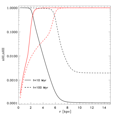
Figure 19: Radial velocity (left) and ionization profiles (right) for an HII expansion test equivalent to Test 5 in Iliev et al. (2009). We show times $t=10$ and $100\,\rm Myr$.

Notice that we do not expect our results to be strongly affected by the sub-optimal performance of the code in shadowing tests, as our science applications of the radiative transfer module deal with spherically symmetric configurations in a homogeneous medium.

A.4 Test 4: classical HII region expansion

This test corresponds to Test 5 suggested in Iliev et al. (2009). Unlike the previous experiments, it studies the dynamical response of the gas to ionization; thus this test is of particular interest for our study. Following Illiev et al., we set up a constant density box with $n_{\rm H}=10^{-3}\,\rm cm^{-3}$ and temperature $T=10^{2}\,\rm K$ where we place a central source emitting at a rate $5\times 10^{48}\,\rm s^{-1}$ photons per second with a $T_{\rm BB}=10^{5}\,\rm K$ black-body spectrum. Iliev et al. originally used a box size of 15 kpc with 128 resolution elements, placing the source in a corner and treating the boundaries of the box as periodic or non-periodic according to their location. For simplicity, we prefer to deal with a central source and treat all boundaries as non-periodic. We therefore use double the size of the box as well as twice the number of cells ($L=30\,{\rm kpc}$ and $256^{3}$, respectively) to match the original numerical resolution.

We find a very good agreement between our results and those in the code comparison paper. For brevity, we show only the velocity and ionization profiles in Fig. 19 for $t=10$ and $100\,{\rm Myr}$, but we have checked that the agreement extends also to the other properties such as temperature, density and pressure profiles.

Summarizing, our code, as all moment-based methods, tends to be too diffusive, despite the efforts to capture the anisotropic propagation of photons. As discussed in PS09, this might affect the geometry of ionized regions in cases where the gas presents a large degree of inhomogeneities. However, apart from this defect, the successful performance of the code in several standard test problems suggests that general properties of the ionized bubbles, such as volume, size, temperature, pressure structure and induced gas dynamics should be properly captured by our scheme.

Appendix B Convergence with number of cells

Fig. 20 shows the numerical convergence of our radiation pressure results with the number of cells. We show the radial velocity measured in the gas for a constant density box with density $n_{\rm H}=1\,\rm cm^{-3}$ and temperature $T=10^{4}\,\rm K$. In general, we use $64^{3}$ cells in our constant density experiments of Sec. 3. Here, we compare $64^{3}$ against the same set-up using $128^{3}$ and $256^{3}$ cells. We find excellent agreement between the curves, indicating that our results are not affected by resolution effects. Notice that, as discussed in the main text, Eq. (9) tends to overestimate the gas velocity at early times. This effect is small, but most importantly, it is independent of our numerical resolution.

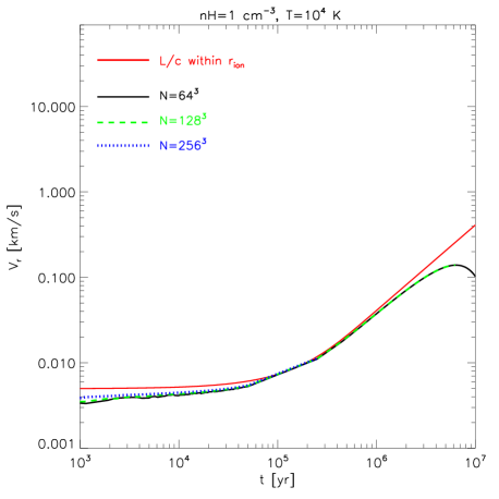
Figure 20: Convergence of the gas velocity with the number of cells, measured in a constant density box with $n_{\rm H}=1\,\rm cm^{-3}$, $T=10^{4}\,\rm K$ and luminosity $L=10^{6}\,\rm L_{\odot}$. The red solid curve indicates the analytical estimate from Eq. (9).

References

- Agertz et al. (2013) Agertz O., Kravtsov A. V., Leitner S. N., Gnedin N. Y., 2013, ApJ, 770, 25
- Arthur et al. (2004) Arthur S. J., Kurtz S. E., Franco J., Albarrán M. Y., 2004, ApJ, 608, 282
- Aubert & Teyssier (2008) Aubert D., Teyssier R., 2008, MNRAS, 387, 295
- Aumer et al. (2013) Aumer M., White S. D. M., Naab T., Scannapieco C., 2013, MNRAS, 434, 3142
- Bauer & Springel (2012) Bauer A., Springel V., 2012, MNRAS, 423, 2558
- Binney & Tremaine (2008) Binney J., Tremaine S., 2008, Galactic Dynamics: Second Edition. Princeton University Press
- Bird et al. (2013) Bird S., Vogelsberger M., Sijacki D., Zaldarriaga M., Springel V., Hernquist L., 2013, MNRAS, 429, 3341
- Castor et al. (1975) Castor J., McCray R., Weaver R., 1975, ApJL, 200, L107
- Cen (1992) Cen R., 1992, ApJS, 78, 341
- Ceverino et al. (2013) Ceverino D., Klypin A., Klimek E., Trujillo-Gomez S., Churchill C. W., Primack J., Dekel A., 2013, ArXiv e-prints 1307.0943
- Dale & Bonnell (2008) Dale J. E., Bonnell I. A., 2008, MNRAS, 391, 2
- Dale et al. (2005) Dale J. E., Bonnell I. A., Clarke C. J., Bate M. R., 2005, MNRAS, 358, 291
- Dale et al. (2012) Dale J. E., Ercolano B., Bonnell I. A., 2012, MNRAS, 424, 377
- Dale et al. (2013) Dale J. E., Ngoumou J., Ercolano B., Bonnell I. A., 2013, MNRAS, 436, 3430
- Dopita & Sutherland (2003) Dopita M. A., Sutherland R. S., 2003, Astrophysics of the diffuse universe
- Gail & Sedlmayr (1979) Gail H. P., Sedlmayr E., 1979, A&A, 77, 165
- Gnedin & Abel (2001) Gnedin N. Y., Abel T., 2001, New Astronomy, 6, 437
- Haehnelt (1995) Haehnelt M. G., 1995, MNRAS, 273, 249
- Harper-Clark & Murray (2009) Harper-Clark E., Murray N., 2009, ApJ, 693, 1696
- Heyer et al. (2009) Heyer M., Krawczyk C., Duval J., Jackson J. M., 2009, ApJ, 699, 1092
- Hopkins et al. (2011) Hopkins P. F., Quataert E., Murray N., 2011, MNRAS, 417, 950
- Iliev et al. (2006) Iliev I. T., Ciardi B., Alvarez M. A., Maselli A., Ferrara A., Gnedin N. Y., Mellema G., Nakamoto T., Norman M. L., Razoumov A. O., Rijkhorst E.-J., Ritzerveld J., Shapiro P. R., Susa H., Umemura M., Whalen D. J., 2006, MNRAS, 371, 1057
- Iliev et al. (2009) Iliev I. T., Whalen D., Mellema G., Ahn K., Baek S., Gnedin N. Y., Kravtsov A. V., Norman M., Raicevic M., Reynolds D. R., Sato D., Shapiro P. R., Semelin B., Smidt J., Susa H., Theuns T., Umemura M., 2009, MNRAS, 400, 1283
- Kim et al. (2013) Kim J.-h., Krumholz M. R., Wise J. H., Turk M. J., Goldbaum N. J., Abel T., 2013, ApJ, 775, 109
- Krumholz & Matzner (2009) Krumholz M. R., Matzner C. D., 2009, ApJ, 703, 1352
- Krumholz et al. (2006) Krumholz M. R., Matzner C. D., McKee C. F., 2006, ApJ, 653, 361
- Krumholz & Thompson (2012) Krumholz M. R., Thompson T. A., 2012, ApJ, 760, 155
- Lagos et al. (2013) Lagos C. d. P., Lacey C. G., Baugh C. M., 2013, MNRAS, 436, 1787
- Levermore & Pomraning (1981) Levermore C. D., Pomraning G. C., 1981, ApJ, 248, 321
- Lopez et al. (2013) Lopez L. A., Krumholz M. R., Bolatto A. D., Prochaska J. X., Ramirez-Ruiz E., Castro D., 2013, ArXiv e-prints 1309.5421
- Marinacci et al. (2014) Marinacci F., Pakmor R., Springel V., 2014, MNRAS, 437, 1750
- Mathews (1969) Mathews W. G., 1969, ApJ, 157, 583
- Matzner (2002) Matzner C. D., 2002, ApJ, 566, 302
- McKee (1989) McKee C. F., 1989, ApJ, 345, 782
- McKee et al. (1984) McKee C. F., van Buren D., Lazareff B., 1984, ApJL, 278, L115
- Muñoz et al. (2013) Muñoz D. J., Springel V., Marcus R., Vogelsberger M., Hernquist L., 2013, MNRAS, 428, 254
- Murray et al. (2005) Murray N., Quataert E., Thompson T. A., 2005, ApJ, 618, 569
- Nelson et al. (2013) Nelson D., Vogelsberger M., Genel S., Sijacki D., Kereš D., Springel V., Hernquist L., 2013, MNRAS, 429, 3353
- Oppenheimer & Davé (2006) Oppenheimer B. D., Davé R., 2006, MNRAS, 373, 1265
- Pakmor & Springel (2013) Pakmor R., Springel V., 2013, MNRAS, 432, 176
- Petkova & Springel (2009) Petkova M., Springel V., 2009, MNRAS, 396, 1383
- Renaud et al. (2013) Renaud F., Bournaud F., Emsellem E., Elmegreen B., Teyssier R., Alves J., Chapon D., Combes F., Dekel A., Gabor J., Hennebelle P., Kraljic K., 2013, MNRAS, 436, 1836
- Rogers & Pittard (2013) Rogers H., Pittard J. M., 2013, MNRAS, 431, 1337
- Sharma et al. (2011) Sharma M., Nath B. B., Shchekinov Y., 2011, ApJL, 736, L27
- Shu (1992) Shu F. H., 1992, The physics of astrophysics. Volume II: Gas dynamics.
- Sijacki et al. (2012) Sijacki D., Vogelsberger M., Kereš D., Springel V., Hernquist L., 2012, MNRAS, 424, 2999
- Spitzer (1978) Spitzer L., 1978, Physical processes in the interstellar medium
- Springel (2005) Springel V., 2005, MNRAS, 364, 1105
- Springel (2010) Springel V., 2010, MNRAS, 401, 791
- Stinson et al. (2013) Stinson G. S., Brook C., Macciò A. V., Wadsley J., Quinn T. R., Couchman H. M. P., 2013, MNRAS, 428, 129
- Torrey et al. (2014) Torrey P., Vogelsberger M., Genel S., Sijacki D., Springel V., Hernquist L., 2014, MNRAS
- Vogelsberger et al. (2013) Vogelsberger M., Genel S., Sijacki D., Torrey P., Springel V., Hernquist L., 2013, MNRAS, 436, 3031
- Vogelsberger et al. (2012) Vogelsberger M., Sijacki D., Kereš D., Springel V., Hernquist L., 2012, MNRAS, 425, 3024
- Walch et al. (2012) Walch S. K., Whitworth A. P., Bisbas T., Wünsch R., Hubber D., 2012, MNRAS, 427, 625
- Whitworth (1979) Whitworth A., 1979, MNRAS, 186, 59
- Wise et al. (2012) Wise J. H., Abel T., Turk M. J., Norman M. L., Smith B. D., 2012, MNRAS, 427, 311
- Yorke et al. (1983) Yorke H. W., Tenorio-Tagle G., Bodenheimer P., 1983, A&A, 127, 313