Probability distributions for Poisson processes with pile-up

Abstract

In this paper, two parametric probability distributions capable to describe the statistics of X-ray photon detection by a CCD are presented. They are formulated from simple models that account for the pile-up phenomenon, in which two or more photons are counted as one. These models are based on the Poisson process, but they have an extra parameter which includes all the detailed mechanisms of the pile-up process that must be fitted to the data statistics simultaneously with the rate parameter. The new probability distributions, one for number of counts per time bins (Poisson-like), and the other for waiting times (exponential-like) are tested fitting them to statistics of real data, and between them through numerical simulations, and their results are analyzed and compared. The probability distributions presented here can be used as background statistical models to derive likelihood functions for statistical methods in signal analysis.

1 Introduction

In the last decades, some statistics methods formulated to find signals in data sets of X-ray astronomy were developed, some of them based on bayesian statistics. For example, Gregory & Loredo (1992) developed a method able to detect and characterize periodical signals of unknown shapes and periods. On the other hand, Hutter (2005) developed a method able to detect changing points on piecewise constant signals, which could, in principle, be used to determine if a source increases abruptly its luminosity, as while a burst. Most of these methods assume a parametric distribution as the background statistical model. Usually, in X-ray astronomy data analysis, the Poisson distribution is used for this purpose, because the process of photon detection is considered as a Poisson process, with a time-dependent rate $r(t)$.

Nevertheless, the process of counting photons in a CCD is not a Poisson process. Some photon counts result lost because of the pile-up effect (Arnaud et al., 2011). Pile-up occurs when two or more photons are collected by the same or adjacent pixels in the same frame, so they result counted as only one event of greater energy.

In this paper, two probability distributions that consider pile-up are introduced. They are obtained independently: one is based on the Poisson distribution, and the other, on the exponential probability density. To prove their validity, they are fitted to real data from RX J0720.4-2125, measured by XMM-Newton EPIC instrument. Also, they are compared to each other through numerical simulations. The results show that the proposed probability distributions describe the statistics of the real data set remarkably well, and they could be used to analyze similar sets of data typically found in X-ray astronomical observations.

The distributions presented in this work could be used to reformulate or improve some of the statistical methods currently used in X-ray astronomy data analysis but do not account for the pile-up effect.

2 X-ray data acquisition and pile-up

For X-ray telescopes working in a frame mode, the data consist of a list of counts where every count ideally corresponds to an arriving photon. These entries have attributes like detection time, photon energy, detection pattern (or grade), $x$ and $y$ pixel coordinates, etc. In this paper we do not discuss the processes of data reduction and selection: we will concentrate our attention only on the arrival time of the detected events (counts), which are supposed to come from a single sky source. All the necessary work to prepare the data we suppose was previously done.

But in practice, some of the arriving photons are not detected by the instrument, that is, do not generate counts. On the other hand, some counts could be not provoked by photons: for example, a count could be provoked by another incoming particle, or even, by an electronic noise.

In general, the arrival of photons to a telescope is a Poisson process: such events are totally independent of one another. The incoming photons are reflected in a focusing system, and then they are collected by a detector, which in this case is a CCD array. But some photons are not reflected in mirrors, and some photons do not interact with CCDs. These two phenomena, which depend on photon energy, are completely stochastic, so they do not break the initial poissonian character of the arriving photons phenomenon, that is, the interaction of photons with the detector (or photon collection) is a Poisson process too. These effects can be described by factors that give the optical and quantum efficiencies (Arnaud et al., 2011). The estimation of the fraction of photons rejected by them is straightforward, but it is out of the scope of the present work.

When an individual photon interacts with a CCD, it makes an electrically charged print in one or more pixels (Ballet, 1999). The CCD collects photons for a time called frame time, which is a fundamental time bin imposed by the instrument. When the frame time finishes, all the pixels are read, and the information of which pixels were charged and their respective amounts of electrical charge, is saved. The reading process takes some time in which the image is moved to the readout register and the collection of photons of sky sources occur in spread areas of the image, so the corresponding counts are usually discarded when the data of a particular sky source are extracted. Then, the reading times can be considered as dead times in which the instrument is blind (time gaps), and so they do not alter the poissonian nature of the photon interaction process.

But there are features of CCD that bias the data and break the poissonian character of the photon counting process: the most important is pile-up. As we stated out earlier, pile-up occurs when, in the same frame, two or more photons hit very close pixels, and they are interpreted as a single event (count). As pile-up is an instrument saturation effect, it is not a Poisson process, so the statistics of counts cannot be properly described by the probability distributions for Poisson processes.

It is important to note that the probability of pile-up depends on the instrument characteristics and the energies of the collected photons. Several authors (Ballet, 1999; Davis, 2001) have studied pile-up making a detailed analysis of the mechanism of grade migration, which is fundamental if the objective is the spectral analysis or the luminosity measure of a stellar source, as pile-up provokes an apparent harder spectrum. But the scope of this work is different: it is to find probability distributions capable to describe the statistics of counts of astronomical X-ray data with no distinction between photon energies. The main purpose of them is to be used as likelihood functions (i.e., as background statistical models) in statistical methods devoted to time-series signal shape characterization, which are commonly used to find periodical pulsations, burst, etc. in stellar light curves. In this way, we will consider all the details of pile-up mechanism described in one parameter, which represents the fraction of counts lost by pile-up.

Finally, the models proposed in this work are essentially different to those that use the one photon approximation, in which it is assumed that not more than one photon can be measured per frame (Kuin, 2008). While this kind of models are devoted to obtain the probability to measure $k$ photons in $N$ frames (being $k\leq N$), the models proposed here follow the purpose to obtain the probability to have $n$ counts in only one frame. On the other hand, the author has no notice of a previous study of the pile-up on a waiting-time probability distribution.

3 Probability distributions

3.1 Probability distributions for Poisson processes

A Poisson process is a stochastic process in which events of a certain kind occur in time independently of one another. In the case analyzed here, such events are the interactions of X-ray photons from a stellar source with the CCD detector of an X-ray telescope. A Poisson process is described by one parameter: the rate of events in time ($r$). There are two parametric probability distributions usually used to describe poissonian processes: the Poisson and the exponential distributions.

3.1.1 Poisson distribution

The Poisson distribution is defined as

$$P_{r,\Delta t}(n)=\frac{(r\,\Delta t)^{n}\>\mathrm{\mathbf{e}}^{-r\,\Delta t}}{n!}$$ (1)

and gives the probability to have a number of detections $n$ in a time interval (i.e., a frame time of the instrument) $\Delta t$, if the rate of detections in time is $r$. It is a discrete distribution, as $n$ can be any natural number or zero. From now on, $\Delta t$ is chosen as the time unit, so the Poisson distribution results

$$P_{r}(n)=\frac{r^{n}\>\mathrm{\mathbf{e}}^{-r}}{n!}$$ (2)

and $r$ will represent the mean number of detections per frame, if the measurement is repeated a large number of times with identical conditions.

3.1.2 Discrete exponential distribution

The exponential distribution is defined as

$$f_{r}(\tau)=r\,\mathrm{\mathbf{e}}^{-r\,\tau}$$ (3)

and it is a probability density distribution, in the sense that

$$\int_{t_{1}}^{t_{2}}f_{r}(\tau)\>d\tau$$

gives the probability to have a waiting time of between $t_{1}$ and $t_{2}$, where waiting time is the elapsed time between two consecutive detections. As the instrument reads at regular time steps $\Delta t$, it is necessary to discretize the exponential distribution in order to use it to analyze a data set. Using again $\Delta t$ as time unit, the probability to obtain a waiting time of $n\>\Delta t$ (or simply $n$), where $n$ can be any natural number or zero, results

$$\left\{\begin{array}[]{l}P_{r}(0)=\int_{0}^{1}(1-t)\>r\>e^{-r\,t}\>dt\\ P_{r}(n)=\int_{n-1}^{n}(1-n+t)\>r\>e^{-r\,t}\>dt+\int_{n}^{n+1}(1+n-t)\>r\>e^{-r\,t}\>dt\end{array}\right.$$ (4)

where the factors in parenthesis are the probabilities of a waiting time of $t$ to be counted as $n$ or $n+1$, being $n<t<n+1$. Equations (4) can be easily integrated

$$\left\{\begin{array}[]{l}P_{r}(0)=1+\frac{e^{-r}-1}{r}\\ P_{r}(n)=\frac{e^{-(n+1)\,r}\left(e^{r}-1\right)^{2}}{r}\end{array}\right.$$ (5)

We will call this probability distribution discrete exponential distribution.

3.2 Distributions for poissonian processes with pile-up

When two or more photons arrive to the detector in the same frame, some of them could be collected on the same place on the CCD, and interpreted as a single count. This effect, which is called pile-up, provokes less counts than the number of collected photons. In this section, probability distributions that consider pile-up are deduced.

3.2.1 Poisson distribution with pile-up

If 2 photons are collected by the CCD in the same frame, there are two possibilities: the second photon can result piled with the first one, or not. Let us call $\alpha_{1}^{1}$ to the probability of the first case, in which the result is only one count. The probability of the second case, where two counts result, is $1-\alpha_{1}^{1}$.

Similarly, if three photons are collected by the CCD in the same frame, there are three possibilities: two counts, one count or none can be lost. Suppose that the second photon results piled with the first one which, as we have seen before, occurs with a probability of $\alpha_{1}^{1}$. When the third photon arrives, the probability of pile-up with the previous count, which was originated by two piled photons, is $\alpha_{1}^{2}$, and the probability of not, is $1-\alpha_{1}^{2}$. In the first case, the result is only one count, and in the second, two counts. Now suppose that the second photon does not result piled with the first one, which occurs with a probability of $1-\alpha_{1}^{1}$. Then, when the third photon arrives, it can result piled with one of the others two, or not. We call $\alpha_{2}^{1}$ to the probability of the first situation, in which the photon results piled with one of the two previous counts, each one originated by one photon, so $1-\alpha_{2}^{1}$ is the probability of the second situation. In the first situation the result is two counts, and in the second one, three counts. The idea can be easily generalized for any number.

Figure 1 shows a tree with the different paths of pile-up in which we can have $n$ counts from $N$ collected photons, up to $N=6$. To calculate the probability of a particular path, we must start from the first column, and pass to the next going to the lower-right node in case of pile-up, or to the upper-right one if pile-up does not occur. We repeat this step until column $N$, which represents the number of photons collected by the CCD. The numbers that label each node are the numbers $n$ of resulting counts. The probability of the path can be obtained multiplying the factors that are pointed out in the arrows that join the nodes. On this way, the sum of the probabilities of all the possible paths that end in the same column is 1.

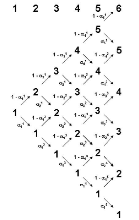
Figure 1: Tree of pile-up possibilities. The column numbers (top numbers) are the numbers of photons collected by the CCD. The numbers on the nodes are the number of counts that the instrument records. For each node, there are different possible paths that end in it. The paths must start in the first node (first column), and follow the arrows. The probability of the paths can be calculated multiplying the factors pointed out in the arrows.

To obtain a formula that expresses the probability of a particular path is not difficult. Dividing that path in $m$ elementary steps that have a segment in the upper-right direction, followed by a segment in the lower-right direction, the probability can be expressed as

$$P_{path}=\prod_{j=0}^{m}\left[\prod_{k=n_{2\,j}+1}^{n_{2\,j+2}}\left(1-\alpha_{k}^{n_{2\,j+1}+1}\right)\>\prod_{k=n_{2\,j+1}+1}^{n_{2\,j+3}}\alpha_{n_{2\,j+2}+1}^{k}\right]$$ (6)

where $n_{0}=n_{1}=0$, and the increments on the even coefficients ($\Delta n_{j}^{u}=n_{2\,j}-n_{2\,j-2}$) and odd coefficients ($\Delta n_{j}^{d}=n_{2\,j+1}-n_{2\,j-1}$) are the numbers of nodes that are crossed in the upper-right and the lower-right directions in the $j^{th}$ step. If the path starts in the lower-right direction, the first step does not have the upper-right segment, and $\Delta n_{1}^{u}$ is 0. If the path ends in the upper-right direction, the last step does not have the segment in the lower-right direction, and $\Delta n_{m}^{d}$ is 0. The other increments must be positive numbers.

Equation (6) is general but too complicated to be useful for pile-up probability calculation. Let us make an assumption to simplify it: let us suppose that

$$\alpha_{k}^{1}=\alpha_{k}^{2}=.....=\alpha_{k}^{n}=\alpha_{k}$$ (7)

Assumption (7) considers that the pile-up probability of a photon that is collected by the CCD only depends on how many counts are already in the frame, but not on if in these counts some of the previous collected photons resulted piled.

To calculate the distribution that gives the probability to obtain $n$ counts considering that the collected photons follow a Poisson distribution, we must add the probabilities of all the nodes $n$. The probability of every node is obtained multiplying the probability $P_{r}(N)$ for the column of the node (where $N$ is the number of collected photons and $P_{r}$ is the Poisson distribution (2)), and the probability obtained adding the probabilities of all the paths that end in that node. After some combinatorial work, the result is

$$P_{r,\left\{\alpha_{1},\alpha_{2},...\right\}}(n)=\sum_{m=0}^{\infty}P_{r}(n+m)\,\left(\sum_{k}\,\prod_{j=1}^{m}b_{k\,j}^{(m)}\right)\,\prod_{i=1}^{n-1}\left(1-\alpha_{i}\right)$$ (8)

where $b_{k\,j}^{(m)}$ is the $j^{th}$ element of the m-tuple $B_{k}^{(m)}$ of the set of the m-tuples of $\left\{\alpha_{1},\alpha_{2},...,\alpha_{n}\right\}$, considering no permutations. Formula (8) is valid for $n\geq 1$. On the other hand, $P_{r,\left\{\alpha_{1},\alpha_{2},...\right\}}(0)$ is equal to $P_{r}(0)$.

The fraction $X$ of lost counts with respect to the total number of collected photons results

$$X_{r,\left\{\alpha_{1},\alpha_{2},...\right\}}=\frac{1}{r}\,\sum_{h,k=0}^{\infty}k\,P_{r}(h+k+1)\,\left(\sum_{l}\prod_{j=1}^{k}b_{l\,j}^{(k)}\right)\,\prod_{i=1}^{k}(1-\alpha_{i})$$ (9)

It is possible to go forward making another assumption on $\left\{\alpha_{k}\right\}$. For a low ratio of counts per frame with respect to the total number of pixels used to acquire the data (i.e. far from saturation), it is a reasonable assumption to take

$$\alpha_{n}=n\,\alpha$$ (10)

This assumption considers that the pile-up probability is proportional to the number of previous counts in the frame. With it, and after more combinatorial work, equation (8) results

$$P_{r,\alpha}(n)=\sum_{j=1}^{\infty}P_{r}(j)\,\alpha^{j-n}\,S_{j}^{(n)}\,\prod_{k=1}^{n-1}\left(1-k\,\alpha\right)$$ (11)

where $S_{j}^{(n)}$ is the Stirling number of second kind. Again, formula (11) is valid for $n\geq 1$. For $n=0$, the probability is $P_{r}(0)$. In this work, this probability distribution is called Poisson distribution with pile-up, despite it is not general.

It is to note that probability distribution (11) is not a Stuttering-Poisson distribution (Galliher et al., 1959). For a Stuttering-Poisson distribution, the probability to obtain the case $n$ from the case $N$ distributed as Poisson, is obtained from the convolution of $N$ indentically distributed random variables. But for distribution (11), the conditional probability $P_{r,\alpha}(n|N)$ is obtained by adding the probabilities of all the possible paths of pile-up, being the probabilities of each step of the paths dependant on the collection history, that is, on the number of counts that already are in the frame. So, the process of photon collection with pile-up is not Stuttering-Poisson, and the probability distribution (11) is not a member of the Stuttering-Poisson class.

An important feature of the function that gives the probability to obtain $n$ counts from $N$ collected photons defined in equation (11)

$$P_{r,\alpha}(n|N)=\alpha^{N-n}\,S_{N}^{(n)}\,\prod_{k=1}^{n-1}\left(1-k\,\alpha\right)$$ (12)

is that it produces alternativelly negative and positive numbers when $n$ is increased beyond certain value which we call $n^{*}$. These values do not correspond to physical probabilities and must be considered as zero, as they are related to the complete saturation of the instrument. The last positive value must be corrected in order to satisfy the normalization condition

$$\sum_{n=0}^{N}P_{r,\alpha}(n|N)=1$$ (13)

Figure 2 shows the graphics of $\log(-p_{r,\alpha}^{*})$ in function of $r$ and $\alpha$, where $p_{r,\alpha}^{*}$ is obtained evaluating equation (11) in $n^{*}$. As we will see in section 6, this procedure is not suitable when $\left|p_{r,\alpha}^{*}\right|\gtrsim 1$ but, as we can see in figure 2, it only occurs when $r$ and $\alpha$ are large.

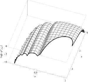
Figure 2: $\log(-p_{r,\alpha}^{*})$ in function of $r$ and $\alpha$. This is the first negative value of equation (11). This value and the successive ones must be considered as zero, and the previous one must be corrected in order to preserve the normalization condition.

Finally, applying assumption (10) to equation (9), and considering its Taylor expansion, it can be proved that the fraction $X$ of lost counts with respect to the total number of collected photons results

$$X_{r,\alpha}=1+\frac{e^{-\alpha\,r}-1}{\alpha\,r}$$ (14)

From equation (14) we can find the highest possible value of $X$ in function of $r$ taking $\alpha=1$

$$X_{max}(r)=1+\frac{e^{-r}-1}{r}$$ (15)

3.2.2 Discrete exponential distribution with pile-up

In this case, when a number $k$ of photons result piled, there is a missing of $k-1$ waiting times equal to 0 in the data set, while the numbers of waiting times different to 0 are the same as they would be if pile-up were null. Calling $X$ to the fraction of lost counts by the pile-up, and considering equation (5), the probability distribution of waiting times taking in account the pile-up results

$$\left\{\begin{array}[]{l}P_{r,X}(0)=\frac{1}{1-X}\,\left(1+\frac{e^{-r}-1}{r}-X\right)\\ P_{r,X}(n)=\frac{1}{1-X}\,\frac{e^{-(n+1)\,r}\left(e^{r}-1\right)^{2}}{r}\end{array}\right.$$ (16)

We will call discrete exponential distribution with pile-up to probability distribution (16). We can see that $P_{r,X}(0)$ is a non negative number only if $X\leq X_{max}(r)$, where $X_{max}(r)$ is the same previously found for the Poisson distribution with pile-up, equation (15).

3.3 Statistical errors

Probability distributions like (11) or (16) express, if a measure is made, the probability to obtain any of the different cases labeled as $n$. Probability distributions also express the fractions of cases $n$ that would be obtained if an infinite number of measures could be made. But the number of measures that can be made is finite so, in general, the fractions $q_{n}$ of the cases $n$ with respect to the total, differ from the probability distribution $P(n)$, being the differences due to chance. Now the typical expected differences, which are called statistical errors, are estimated.

If the probability of happening for the case $n$ in a measure is $P(n)$, then the probability of not happening is $1-P(n)$. If the experiment is repeated $N$ times, the probability to obtain $Q_{n}$ times the case $n$ can be estimated through the binomial distribution. The most probable number of times in which the event $n$ occurs is $N\,P(n)$, being the variance $N\,P(n)\,(1-P(n))$. As $N$ usually is a large number, there is not a significant difference between the binomial distribution and the normal distribution with the same mean value and variance. From this, we can estimate the typical differences between data statistics $q_{n}=Q_{n}/N$ with respect to their most probable expected values $P(n)$ through the standard errors of the related normal distributions, that is, the square roots of the variances

$$\sigma_{n}=\sqrt{\frac{P(n)\,\left(1-P(n)\right)}{N}}$$ (17)

Equation (17) is good enough to estimate the statistical errors for $P(n)>5/N$ (Box, 1978). In that case, it is expected that $\left|q_{n}-P(n)\right|$ be less than $\sigma_{n}$ for the 68 % of the cases, less than $2\,\sigma_{n}$ for the 95% of the cases, and less than $3\,\sigma_{n}$ for the 99.7% of the cases.

4 Pile-up estimation and rate of photon collection

In sections 3.2.1 and 3.2.2 two probability distributions able to describe the statistics of data sets of counts obtained from an intrinsic poissonian process, like the arrival of photons to an X-ray telescope focal plane, measured by an instrument which shows pile-up, like a CCD, were deduced. Now, the problem of how to find the set of parameters that make the best fit of a probability distribution (statistical model) with respect to the statistics of a given data set is treated.

Consider the probability distribution $P_{r,s}(n)$ that could be (11) or (16), so $s$ represents $\alpha$ or $X$. To find the best fitting parameters, the least squares method can be used. This method consists of finding the values of the parameters that minimize the quantity

$$\chi^{2}(r,s)=\sum_{n=0}^{n_{max}}\frac{\left(P_{r,s}(n)-q_{n}\right)^{2}}{\sigma_{n}^{2}}$$ (18)

where $\sigma_{n}$ is given by equation (17). The upper limit of the sum, $n_{max}$, which in theory is infinity, in practice is a number that satisfies, on one hand, that $q_{n}=0$ for $n>n_{max}$, and on the other, that $P_{r,s}(n_{max}+1)\ll 1/N$, being $N$ the number of elements of the data set.

If the probability distribution used to fit the data statistics is able to describe them, then the statistics of $\chi^{2}(r,s)$ defined in equation (18) must be chi-square distributed, with $n_{max}-1$ degrees of freedom (Wall & Jenkins, 2003). This is a consequence of the normally and independently distributed statistical errors of equation (17).

To determine the statistical errors of the coefficients $\mathbf{a}=(r,s)$, the Taylor expansion of $\chi^{2}(r,s)$ around its minimum is used

$$\chi^{2}(\mathbf{a}+\delta\mathbf{a})=\chi_{min}^{2}+\delta\mathbf{a}^{T}\>\mathbf{H}(\mathbf{a})\>\delta\mathbf{a}$$ (19)

where $\mathbf{H}$ is the Hessian of $\chi^{2}$, and its components are equal to (Richter, 1995)

$$H_{j\,k}(\mathbf{a})=\sum_{n=0}^{n_{max}}\frac{1}{\sigma_{n}^{2}}\,\left.\frac{\partial P_{r,s}(n)}{\partial a_{j}}\right|_{\mathbf{a}}\,\left.\frac{\partial P_{r,s}(n)}{\partial a_{k}}\right|_{\mathbf{a}}$$ (20)

If $\mathbf{C}(\mathbf{a})=\mathbf{H}^{-1}(\mathbf{a})$, the variance of the parameters result

$$\sigma_{r}^{2}=\left|\mathbf{C}(\mathbf{a})_{11}\right|$$ (21)

$$\sigma_{s}^{2}=\left|\mathbf{C}(\mathbf{a})_{22}\right|$$ (22)

The square roots of these quantities ($\sigma_{r}$ and $\sigma_{s}$) are the standard errors of the parameters $r$ and $s$ estimated through the least squares method.

Now, let us consider the effective rate of counts $r_{m}$ measured by the instrument. It is related to $r$ and $X$ through

$$r_{m}=(1-X)\,r$$ (23)

Equation (23) is useful to check the consistency of the results, and it can also be used to improve the estimations of $r$ and $X$. As (23) permits to obtain $r(X)$ and $X(r)$, it is possible to promediate $r$ with $r(X)$ and $X$ with $X(r)$, with relative weights according to their statistical errors (Wall & Jenkins, 2003). Calling $\hat{r}$ and $\hat{X}$ to these corrected values, they result

$$\frac{\hat{r}}{\sigma_{\hat{r}}^{2}}=\frac{r}{\sigma_{r}^{2}}+\frac{(1-X)^{3}}{r_{m}}\,\frac{1}{\sigma_{X}^{2}}$$ (24)

$$\frac{\hat{X}}{\sigma_{\hat{r}}^{2}}=\frac{X}{\sigma_{X}^{2}}+\left(\frac{r^{4}}{r_{m}^{2}}-\frac{r^{3}}{r_{m}}\right)\,\frac{1}{\sigma_{r}^{2}}$$ (25)

where $\sigma_{\hat{r}}$ and $\sigma_{\hat{X}}$ are the standard errors of $\hat{r}$ and $\hat{X}$

$$\frac{1}{\sigma_{\hat{r}}^{2}}=\frac{1}{\sigma_{r}^{2}}+\frac{(1-X)^{4}}{r_{m}^{2}}\,\frac{1}{\sigma_{X}^{2}}$$ (26)

$$\frac{1}{\sigma_{\hat{r}}^{2}}=\frac{1}{\sigma_{X}^{2}}+\frac{r^{4}}{r_{m}^{2}}\,\frac{1}{\sigma_{r}^{2}}$$ (27)

For the case of the discrete exponential distribution with pile-up (16), $X$ and $\sigma_{X}$ are obtained directly from least squares method and equation (22), because $X$ is one of the parameters of the distribution. But, for the case of the Poisson distribution with pile-up (11), $X$ is a function of parameters $r$ and $\alpha$, so $\sigma_{X}$ must be obtained propagating the errors $\sigma_{r}$ and $\sigma_{\alpha}$ in the function (14)

$$\sigma_{X}^{2}=\left(\frac{\partial X_{r,\alpha}}{\partial r}\right)^{2}\,\sigma_{r}^{2}+\left(\frac{\partial X_{r,\alpha}}{\partial\alpha}\right)^{2}\,\sigma_{\alpha}^{2}$$ (28)

5 Application to real data

5.1 RX J0720.4-3125

As application example, a data set from an observation of RX J0720.4-3125 is analyzed. This X-ray source is an isolated and radio-quiet neutron star. Its luminosity is apparently due to thermical emission, and it is very regular in an observation-time, except for a periodic change of about 20% in its intensity due to its rotation, with a period of approximately 8.39 s (Hohle et al., 2010). Also, there is no evidence of short-time luminosity variations, like sub-second bursts (Sevilla 2013, in preparation). Figure 3 shows the mean count rate $r_{m}$ measured by the instrument (see section 5.2) for 20 different star phases, obtained by time folding method (Lorimer & Kramer, 2005). The points are connected by lines for a better visualization.

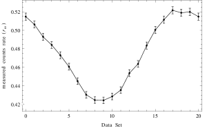
Figure 3: Mean count rate per time bin ($\sim 73$ ms) measured from RX J0720.4-3125 by EPIC pn instrument at XMM-Newton Observatory on 2000 May 13. The data were folded in time in 20 bins per period of $\sim$8.39 s. The curve is similar to the light curve of the star, but the abscissas are labeled in data set number instead of star phase.

5.2 Data

The data set used was obtained by EPIC pn instrument at XMM-Newton observatory, operating in full frame mode, with a time resolution of about 73.4 ms. It corresponds to a continuous observation (without gaps) of approximately 29.2 ks, extracted from good time intervals of observation ID 0124100101 on 2000 May 13.

The time bins in data are not regular, because they are expressed in universal time instead of on-board time, but they can be considered as equal, as the relative difference between the longest and the shortest is less than $6\times 10^{-4}$, too small to be significant. The cumulative differences between the universal times of the events and the times obtained considering a regular time bin result be less than 0.13 time bin, that is, less than $0.01\>\mathrm{s}$. These differences are negligible compared to the period of the star, so the time transformation does not provoke an appreciable phase shift. Finally, only events of between 120 and 1000 eV are considered. It is because a very low flux of photons from the source out of this range is expected.

5.3 Statistics of data

As the luminosity of the star is periodic, different subsets of data close to a given star phase were considered, in order to obtain sets of data of quasi-constant luminosity. For that, the 10 closest time bins per period for 20 different and equal spaced phases were selected, obtaining 20 different data subsets of almost constant luminosities. Two different lists for every data subset were created: one listing every time bin and its number of counts, and the other listing the differences of time between every count and its previous one. Then, for each list, the fractions $q_{n}$ of cases labeled as $n$ with respect to the total were calculated. These sets $\{q_{n}\}$ (for counts per time bin and for waiting times), together with the mean rate of counts per time bin $r_{m}$, are the statistics needed for every subset of data. The subsets are sequentially labeled from 1 to 20 (subsets 0 and 20 are the same) and, in all this work, the number of subset is used to refer to a particular subset instead of its corresponding star phase.

Figure 4 shows the statistics of measured counts per time bin for the 20 data subsets (gray squares). It also shows the Poisson distributions for the highest and the lowest measured count rates showed in figure 3 (black circles). Points are connected by lines for a better visualization. These graphics clearly show that there are less time bins with multiple counts in the data subsets than the number that the Poisson distributions for the extreme values of $r_{m}$ predict.

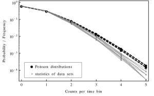
Figure 4: Comparison of Poisson distributions (black circles) with the statistics of data for the 20 subsets (gray squares). For the probability distributions, the highest and the lowest measured mean rates of counts per time bin $r_{m}$ were considered (see figure 3).

Figure 5 shows the statistics of waiting times for the 20 data subsets (gray squares). It also shows the discrete exponential distributions for the highest and the lowest measured count rates showed in figure 3 (black circles). Again, the points are connected by lines for a better visualization. These graphics clearly show that there are fewer cases of waiting time 0 than the number that the discrete exponential distributions for the extreme values of $r_{m}$ predict.

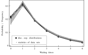
Figure 5: Comparison of discrete exponential distributions (black circles) with the statistics of data for the 20 subsets (gray squares). For the probability distributions, the highest and the lowest measured mean rates of counts per time bin $r_{m}$ were considered (see figure 3).

5.4 Pile-up estimation and rate of photon collection

In this section, the probability distributions with pile-up deduced in section 3.2 are fitted to the statistics of the data subsets, and their parameters are estimated. Poisson and discrete exponential distributions with pile-up are treated separately, and finally, their results are compared.

5.4.1 Poisson distribution with pile-up

Parameters $r$ and $\alpha$ for the best fit of probability distribution (11) to the 20 data subsets obtained in section 5.2 were estimated. It was done calculating $\chi^{2}$ through equation (18) for different values of these parameters, and selecting those that make $\chi^{2}$ minimum. Plots of $\chi^{2}$ show that it has a quadratic-like behavior in the minimum neighborhood, so the procedure is justified.

The parameters were considered in the ranges $0.4\leq r\leq 0.8$ and $0.001\leq\alpha<\alpha_{max}$ with steps of $0.001$. The limit $\alpha_{max}$ was chosen as the minor value of $\alpha$ that makes $P_{r,\alpha}(n)$ equal to one, for which $\chi^{2}$ has a singular point, which is related to the complete saturation of the instrument.

Figure 6 shows the rate of photon collection per time bin estimated directly through parameter $r$ (in black), and from $X_{r,\alpha}$ through equation (23) (in gray), for the 20 different data subsets. The points are joined by lines for a better visualization. It also shows their respective error bars. As we can see, both curves are practically coincident, being the differences consistent with their respective statistical errors.

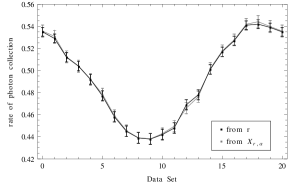
Figure 6: Estimation of the rates of photon collection per time bin for the 20 data subsets fitting the Poisson distribution with pile-up to the data statistics of counts per time bin. Black points indicate the estimations using only parameters $r$ and gray points indicate the estimations using only the values of the fractions of lost counts $X_{r,\alpha}$.

Figure 7 shows the fraction of lost counts obtained from $r$ through equation (23) (in black), and from $r$ and $\alpha$ through equation (14) (in gray), for the 20 data subsets. The points are joined by lines for a better visualization. It also shows their respective error bars. Again, we can see that the agreement between both curves is very good, being the differences consistent with the estimated statistical errors. It is interesting that the fraction of lost counts seems to have a variation with respect to the subset number, and then, to the star phase. This variation is expected, and it is related to the rate of photon collection: the greater the rate of photon collection, the greater the fraction of counts lost by the pile-up.

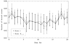
Figure 7: Estimation of the fractions of counts lost by pile-up for the 20 data subsets fitting the Poisson distribution with pile-up to the data statistics of counts per time bin. Black points indicate the estimation using only parameter $r$ and gray points indicate the estimation using only $X_{r,\alpha}$.

Figure 8 shows the estimated $\alpha$ for the 20 data subsets. The points are connected by lines for a better visualization, and the error bars are shown. It is interesting that the values of $\alpha$ do not show an appreciable variation that could be related to the rate of photon collection. Particularly, around the ninth subset, which corresponds to the minimum rate of photon collection (figure 6), the value of $\alpha$ is close to its mean value for all the subsets. It has a simple explanation: while $X$ is expected to be dependent on $r$ (the greater the mean number of photons collected in a frame, the greater the pile-up), $\alpha$, that expresses the probability of pile-up of a photon with respect to one previous count in a frame, is not.

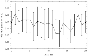
Figure 8: Estimation of the parameter $\alpha$ that represents the probability of pile-up of a photon which is collected from a frame with already one count, for the 20 subsets. The estimations were made fitting the Poisson distribution with pile-up to the data statistics of counts per time bin.

Figure 9 shows the statistics of measured counts per time bin for the 20 data subsets (gray squares), and the Poisson distributions with pile-up for the highest and the lowest values of parameter $r$ showed in figure 6, and the respective values of parameter $\alpha$ (black circles). Points are connected by lines for a better visualization. These graphics show a good agreement between the probability distributions and the statistics, until 4 counts per time bin. But, the agreement is also good for 5 counts per time bin: it is only the logarithmic scale in $y$ axis what magnifies the differences. As the data subsets have approximately 34,700 time bins, the expected number of bins with 5 counts is only one. In fact, in 8 of the 20 data subsets, there is only one time bin with 5 counts. The numbers of subsets in which times bins with 5 counts are present 2, 3 and 4 times are 5, 3 and 2, respectively. Finally, there are 2 data subsets with no bins with 5 counts. These last cases are not shown in figure 10, because they correspond to a frequency of $10^{-\infty}$.

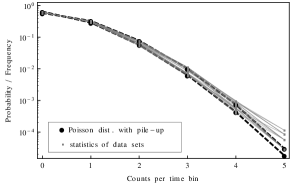
Figure 9: Comparison of Poisson distributions with pile-up (black circles), with data statistics of counts per time bin for the 20 subsets (gray squares). For the probability distributions, the highest and the lowest values of the parameter $r$ were considered (figure 6), and their corresponding values of $\alpha$ (figure 8).

Figure 10 shows the differences between the statistics numbers for the 20 data subsets with respect to the probabilities given by their corresponding fitting Poisson distributions with pile-up, normalized to the standard errors ($\sigma_{n}$). It is evident that the differences are of the order of the statistical errors for all the cases $n$. Nevertheless, we can see systematic differences of the order of their standard errors, specially for the cases of 1 and 2 counts per time bin. But these differences, which are probably due to the assumptions (7) and (10) introduced to simplify the probability distribution expression, are not very important, and the fitting between the probability distributions and the statistics are quite good.

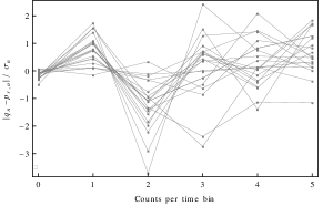
Figure 10: Differences between the statistics of counts per time bin and the probabilities given by the Poisson distributions with pile-up that fit to them, for the 20 data subsets. The differences are normalized to the standard error $\sigma_{n}$.

Finally, figure 11 show an histogram of $\chi^{2}(r,\alpha)$ for the 20 data subsets, and the corresponding probabilities obtained from the chi-square distribution with 5 degrees of freedom, with their respective error bars. The width of the histogram bars was choosen as 5 in order to have some cases in most of the intervals. The corresponding probabilities were obtained integrating the chi-square distribution on these intervals. We can see that the agreement between the statistics of $\chi^{2}(r,\alpha)$ for the 20 subsets, and the probabilities given by the chi-square distribution, is fair. The statistics of $\chi^{2}(r,\alpha)$ seem to be more widely dispersed than the values for the probabilities given by the chi-square distribution. It is due to the systematic differences stated before (see figure 10). Nevertheless, the fitting can be considered as good, so the Poisson distribution with pile-up appears to be a reasonable statistical model to describe the statistics of the data subsets.

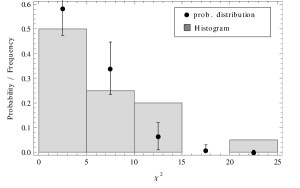
Figure 11: Comparison between the $\chi^{2}(r,\alpha)$ statistics for the 20 data subsets (histogram) and the probable number of cases for the same intervals calculated with the chi-square distribution with 5 degrees of freedom (black circles).

5.4.2 Discrete exponential distribution with pile-up

Again, $\chi^{2}$ was calculated for every data subset, for a range of $0.2<r<0.8$ and $0.001<X<0.5$, with steps of 0.001, and the values for the minimum were selected. Again, plots of $\chi^{2}$ show a good behavior (quadratic-like) that justified the employed method.

Figure 12 shows $r$ (black points) and $r_{m}/(1-X)$ (gray points) for the 20 different data subsets. The points are joined with lines, and their respective error bars are also shown. We can see that the agreement between both quantities is very good, and the differences are of the order of the estimated statistical errors.

Figure 12: Estimation of the rates of photon collection per time bin for the 20 data subsets fitting the discrete exponential distribution with pile-up to the data statistics of waiting times. Black points indicate the estimations using only parameters $r$ and gray points indicate the estimations using only the values of the fractions of lost counts $X$.

Figure 13 shows $X$ (gray points) and $1-r_{m}/r$ (black points), with their respective error bars, for the 20 different data subsets. The points are joined with lines. Again, we can see that the agreement between both quantitites is quite good, compatible with the estimated statistical errors. As in figure 7, $X$ shows a variation for the different data subsets, according to the value of $r$. As it was explained in the previous section, this variation is expected and has a physical explanation.

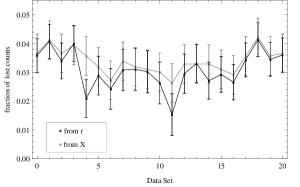
Figure 13: Estimation of the fractions of counts lost by pile-up for the 20 data subsets fitting the discrete exponential distribution with pile-up to the data statistics of waiting times. Black points indicate the estimation using only parameter $r$ and gray points indicate the estimation using only $X$.

Figure 14 shows the statistics $q_{n}$ of the measured waiting times for the 20 data subsets (gray squares), and the discrete exponential distributions with pile-up $P_{r,X}(n)$ for the highest and the lowest values of parameter $r$ showed in figure 12, and their respective values of $X$ (black circles). Points are connected by lines for a better visualization. We can see that the agreement between the probability distributions and the statistics is very good for all the points.

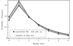
Figure 14: Comparison of discrete exponential distributions with pile-up (black circles), with data statistics of waiting times for the 20 subsets (gray squares). For the probability distributions, the highest and the lowest values of the parameter $r$ were considered (figure 12), and their corresponding values of $X$ (figure 13).

Figure 15 shows the differences between the statistics $q_{n}$ for the 20 data subsets with respect to the probabilities $P_{r,X}(n)$ given by the discrete exponential distributions with pile-up that best fit to them, normalized to their respective standard errors $\sigma_{n}$ (17). Again, we can see that the differences are of the order of the statistical errors. In this case, if there are systematic differences, they are not evident. The explanation is that, unlike for the Poisson distribution with pile-up, for the discrete exponential distribution with pile-up no assumptions are needed to arrive to a final expression depending on two parameters: expression (5) depends on two parameters from the beginning.

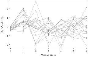
Figure 15: Differences between the statistics of waiting times and the probabilities given by the discrete exponential distributions with pile-up that fit to them, for the 20 data subsets. The differences are normalized to the standard error $\sigma_{n}$.

Finally, figure 16 shows an histogram of $\chi^{2}(r,\alpha)$ for the 20 data subsets, and the corresponding probabilities obtained from the chi-square distribution with 6 degrees of freedom. The width of the histogram bars was choosen as 5, and the corresponding probabilities were obtained integrating the chi-square distribution on those intervals. Now, we can see that the agreement between the $\chi^{2}(r,\alpha)$ statistics for the 20 subsets and the probabilities given by the chi-square distribution is very good. These results indicate that the discrete exponential distribution with pile-up is a good statistical model to describe the statistics of the data subsets.

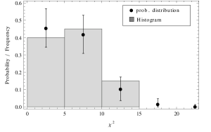
Figure 16: Comparison between the $\chi^{2}(r,X)$ statistics for the 20 data subsets (histogram) and the probable number of cases for the same intervals calculated with the chi-square distribution with 6 degrees of freedom (black circles).

5.4.3 Comparison of results

In sections 5.4.1 and 5.4.2 the consistency of the obtained results for each probability distribution were checked separately. Now, the comparison of the results for both probability distributions is made.

Figure 17 shows the results of the rate of collected photons obtained by the Poisson distribution with pile-up (black points) and by the discrete exponential distribution with pile-up (gray points). The points are joined with lines for a better visualization. The values were obtained through equation (24), which gives an improved value of them combining the results for the two parameters of each distribution. Error bars are also shown

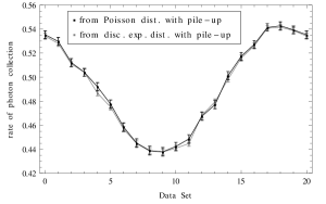
Figure 17: Rate of photon collection per time bin obtained fitting data statistics of counts per time bin to Poisson distribution with pile-up (black points), and statistics of waiting times to discrete exponential distribution with pile-up (gray points).

We can see that the agreement of the mean value of collected photons per time bin calculated from both probability distributions is very good, and the small differences they show can be explained by the statistical errors.

Finally, figure 18 shows the results of the fraction of lost counts obtained by the Poisson distribution with pile-up (black points) and the discrete exponential distribution with pile-up (gray points). The points are joined by lines for a better visualization. The used values were obtained from equation (25). Error bars are also shown. Again, we can see a very good agreement between the values obtained from both distributions.

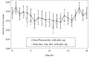
Figure 18: Fraction of lost counts obtained fitting data statistics of counts per time bin to Poisson distribution with pile-up (black points), and statistics of waiting times to discrete exponential distribution with pile-up (gray points).

6 Tests with simulated data

In the previous section, the probability distributions proposed in this work were used to characterize the statistics of a set of real X-ray astronomical data. These two probability distributions, which arise from completely different models, were fitted to the statistics of data, allowing to obtain the rate of photon collection and the fraction of lost counts, being the results for both probability distributions consistent. In this section, the two probability distributions are compared to each other for different values of parameters through numerical simulations. The aim is to explore when the probability distributions show consistent results.

6.1 Method

First, it is important to note that tests with real data can be more decisive than tests with simulated data, because to simulate data it is necessary to use a model. If the model used for simulations were related (i.e. has similar assumptions) to the model used in the method to analyze, the results of the tests could be a non appropriate validation. Fortunately, in this work, two different probability distributions, which arise from completely independent models, are presented, so it is possible to confront them with no danger of obtaining false positive results. The two probability distributions were confronted as follows: sets of data obtained through numerical simulations using one probability distribution (say A), were analyzed with the other one (say B), in order to see the capability of probability distribution B to fit on the corresponding statistics of data sets stochastically distributed as probability distribution A. As the statistical errors of the procedure depend not only on fittings but also on simulations, for the estimation of the quality of the fittings of B in data sets generated with A, fittings of probability distribution A on the same data sets were made. In this way, the capability of probability distribution B to fit on the corresponding statistics of the data sets can be seen by comparison.

To simulate a set of data using a probability distribution, first, this probability distribution is truncated in its last relevant value $p_{M}$. The criterion to determine this value is $p_{M}\lesssim 1/N$, where $N$ is the number of elements of the data set that will be generated. Then, a random number $x$ between 0 and 1, with more precision than the magnitude of $p_{M}$, is generated. In this work, $p_{M}\lesssim 10^{-4}$, and the random numbers were generated using the RandomReal function of Wolfram Mathematica, with a working precision of 6 (i.e., with 6 digits of precision). Next, the random number $x$ is compared to $p_{M}$. If it results lower than $p_{M}$, the number $M$ is added to the data set. But if $x$ results greater than $p_{M}$, then it is compared to $p_{M}+p_{M-1}$, adding the value $M-1$ to the data set if $x$ results lower than that value. If it were necessary, the same procedure is repeated until one of the numbers $M$, $M-1$, … , 1, 0 results added to the data set, with probabilities $p_{M}$, $p_{M-1}$, … , $p_{1}$, $p_{0}$, respectively. Then, the data set is transformed into a list of waiting times (or of counts per time bin, if the simulation were made with the discrete exponential distribution with pile-up), and the statistics ${q_{n}}$ are calculated for both lists. The analysis of the data sets with the probability distributions were made by searching the parameters that make the best fitting of them on the corresponding statistics of the data sets. The procedure used to find the best fitting parameters was to minimize the quantity $\chi^{2}$, equation (18). It was done using the function FindMinimum of the software Wolfram Mathematica. In this way, from the parameters used in simulations ($r_{sim}$, $\alpha_{sim}$ for the Poisson distribution with pile-up, and $r_{sim}$, $X_{sim}$ for the discrete exponential distribution with pile-up), the parameters $r_{fit}$, $\alpha_{fit}$, and $r_{fit}$, $X_{fit}$ that make the best fits of both probability distributions on the respective statistics of the data sets could be obtained, and then compared.

6.2 Results

Several sets of data obtained through the Poisson distribution with pile-up, with parameters $r_{sim}$, $\alpha_{sim}$ varying between $r_{min}=0.01$, $r_{max}=5$ and $\alpha_{min}=0.01$, $\alpha_{max}=0.99$ were simulated. For every choice of parameters, 10 simulations of $10^{4}$ counts were made. Then, the parameters $r_{fit}$ and $X_{fit}$ that make the best fit of the exponential distribution with pile-up on the statistics of waiting times were obtained.

The parameters obtained by fitting were compared to the ones used as input in the simulations. It was done using the folowing parameter

$$\epsilon_{r}=\frac{r_{sim}-r_{fit}}{r_{sim}-r_{m}}$$ (29)

that gives the ratio of the difference between the rates of photon collection used in simulation and obtained by fitting, with respect to the difference between the rate of photon collection used in simulation and the statistic $r_{m}$, that is, the rate of lost counts. It is possible to make a similar analysis with the parameter $X$, but the results are quite similar, as both parameters are related trough $r_{m}$ (see equation (23)). As the denominator of equation (29) is approximately $X\,r_{sim}$ (where $X$ is $X(r_{sim},\alpha_{sim})$ or $X_{sim}$, depending on which probability distribution is used on simulation), it is convenient to use $X\,\epsilon_{r}$ for the analysis, in order to have approximately the same dispersion of values for different parameters.

Figure 19 shows the graphics of $X\,\epsilon_{r}$ for the discrete exponential distribution with pile-up in function of $r_{sim}$ and $\alpha_{sim}$. We can see that the values are close to 0. For large values of $r$ and $\alpha$, there is a zone in which the fittings usually fail. In that zone $\left|p^{*}\right|\gtrsim 1$ (see figure 2).

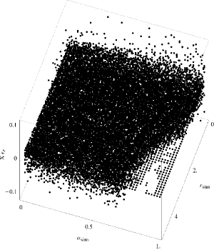
Figure 19: $X\,\epsilon_{r}$ for $r_{fit}$ obtained by fitting the discrete exponential distribution with pile-up on statistics of data sets obtained by simulation using the Poisson distribution with pile-up, in function of the simulation parameters $r_{sim}$ and $\alpha_{sim}$.

Figure 20 shows the graphics of $X\,\epsilon_{r}$ for the Poisson distribution with pile-up, the same used in simulations. We can see that the dispersion of values seems similar to the obtained in the previous case. Figure 21 shows the distributions of the values of $X\,\epsilon_{r}$ for both fittings. We can see that the dispersion is quite similar for both cases. It shows that the discrete exponential distribution with pile-up results an excellent statistical model to describe sets of data stochastically distributed as the Poisson distribution with pile-up.

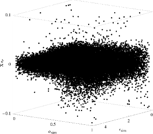
Figure 20: $X\,\epsilon_{r}$ for $r_{fit}$ obtained by fitting the Poisson distribution with pile-up on statistics of data sets obtained by simulation using the same probability distribution, in function of the simulation parameters $r_{sim}$ and $\alpha_{sim}$.

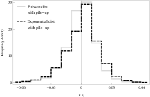
Figure 21: Distributions of the values of $X\,\epsilon_{r}$ obtained by fitting the discrete exponential distribution with pile-up (see figure 19) in black dashed line, and the Poisson distribution with pile-up (see figure 20) in gray continuous line, on the corresponding statistics of data sets obtained by simulation using the Poisson distribution with pile-up.

The same procedure was applied to test the capability of the Poisson distribution with pile-up to describe the statistics of data sets generated through the exponential distribution with pile-up. For several pairs of parameters $r_{sim}$, $X_{sim}$ varying between $r_{min}=0.01$, $r_{max}=5$ and $X_{min}=0.01$, $X_{max}=X_{max}(r)$ (equation (15)), 10 simulations of $10^{4}$ events were made. The parameters $r_{fit}$ and $\alpha_{fit}$ that make the best fit of the Poisson distribution with pile-up on the statistics of counts per frame were obtained. Figure 22 shows $X_{sim}\,\epsilon_{r}$ in function of $r_{sim}$ and $X_{sim}$. In this case, we can see that there are several points with large values of $\epsilon_{r}$, and they seem to be not uniformlly distributed around 0.

Figure 22: $X\,\epsilon_{r}$ for $r_{fit}$ obtained by fitting the Poisson distribution with pile-up on statistics of data sets obtained by simulation using the discrete exponential distribution with pile-up, in function of the simulation parameters $r_{sim}$ and $X_{sim}$.

Figure 23 shows $X_{sim}\,\epsilon_{r}$ in function of $r_{sim}$ and $X_{sim}$ for the same sets of data, but now fitted by the discrete exponential distribution with pile-up, which is the same probability distribution used in simulations. Now we can see that the values of $X_{sim}\,\epsilon_{r}$ are close to 0, and they seem to be uniformlly distributed around this value.

Figure 23: $X\,\epsilon_{r}$ for $r_{fit}$ obtained by fitting the discrete exponential distribution with pile-up on statistics of data sets obtained by simulation using the same probability distribution, in function of the simulation parameters $r_{sim}$ and $X_{sim}$.

Figure 24 shows the distributions of the values of $X_{sim}\,\epsilon_{r}$ obtained by fitting both probability distributions on the sets of simulated data. In this case we can see a notorious difference between both distributions. While the values for the discrete exponential distribution with pile-up seem to have a symetrical distribution around 0, the values for the Poisson distribution with pile-up present a wider distribution which is not symetrical.

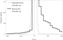
Figure 24: Distributions of the values of $X\,\epsilon_{r}$ obtained by fitting the Poisson distribution with pile-up (see figure 22) in black dashed line, and the discrete exponential distribution with pile-up (see figure 23) in gray continuous line, on the corresponding statistics of data sets obtained by simulation using the discrete exponential distribution with pile-up.

Although there are a large number of cases in which the fittings are good, there are a significative number of situations in which the fittings are not satisfactory. This behaviour points out that the model of the Poisson distribution with pile-up is more restrictive than the model of the discrete exponential distribution with pile-up, in the sense that there are sets of data whose statistics can be described by de second one, but not by the first one.

6.3 Conclusions

The tests with simulated data show that the Poisson distribution with pile-up and the discrete exponential distribution with pile-up do not describe different aspects of the same phenomenon, as the Poisson and Exponential distribution do for a Poisson process, in the sense that statistics of sets of data stochastically generated with one of them can be described by the other one and vice versa. In fact, the discrete exponential distribution with pile-up is able to describe the statistics of a set of data stochastically generated through the Poisson distribution with pile-up for a wide domain, but the opposite is not true. It has a simple explanation: while the model used for the formulation of the discrete exponential distribution with pile-up only assumes that a fraction of waiting times equal to 0 is lost (which basically is the fundamental feature of pile-up phenomenon), the Poisson distribution with pile-up proposed here relies on two arbitrary assumptions (equations 7 and 10) which are expected to be good aproximations to the behaviour of real detectors for low values of $r$ and $\alpha$, but they could be replaced by other ones and still satisfying the model of the discrete exponential distribution with pile-up. So, the discrete exponential distribution with pile-up corresponds to a more general model, and it is able to describe the statistics of a whole class of models which includes the corresponding to the Poisson distribution with pile-up presented in this paper.

7 Summary and discussion

In this paper, two different probability distributions for the description of statistics of data obtained from measurements of a poissonian process by an instrument that presents pile-up are deduced. These probability distributions give the probability to have a number of counts per time bin, or a certain waiting time between consecutive counts, and they were deduced from the Poisson and the exponential distributions. We call these probability distributions Poisson distribution with pile-up and discrete exponential distribution with pile-up.

A general form of the Poisson distribution with pile-up is complicated, because it must depend on several parameters, some of them impossed by the instrument used in data acquisition and the photon energy spectrum. But, through two assumptions, which are expected to be good approximations for low rates of photon collection, a simple analytical expression depending on only two parameters can be obtained (equation 11), being this expression independent from instrument features. These parameters represent the rate of collected photons per time ($r$), and the probability of pile-up of a collected photon with a previous count ($\alpha$). But its validity depends on the validity of the assumptions, so it is not general.

The discrete exponential distribution with pile-up results very simple. The obtained formula depends on only two parameters: $r$ (the mean number of collected photons per time bin) and $X$ (the fraction of lost counts) from the beginning, so no extra assumptions were needed. Then, this distribution results to be general, and so, valid for any pile-up situation over a poissonian process. In that sense, the discrete exponential distribution with pile-up is more simple and robust than the Poisson distribution with pile-up. Nevertheless, in X-ray data analysis, the Poisson distribution is widely used, but the exponential distribution, rarely is.

To check the validity of the probability distributions presented here, first, they were fitted to the same data set using the least squares method, and their results were analyzed and compared. To do that, a set of real astronomical data was used. It was obtained from the isolated neutron star RX J0720.4-3125 by EPIC pn instrument at XMM-Newton Observatory. The fittings on the statistics of data result very good for both distributions, and the estimations of the mean rates of photon collection, and the fraction of lost counts, result consistent and practically coincident. So, it can be concluded that the proposed probability distributions are valid to describe the statistics of the data of this particular observation, and it is reasonable to think that they can be valid to describe other cases similar to this.

Also, the two probability distributions were tested between them through numerical simulations. To do that, one of them was used to generate sets of data for different values of parameters, and the other probability distribution was fitted to the statistics of the data sets, in order to find the values of its parameters that describe them best. Then, the values of parameters obtained fitting the second probability distribution were compared to the parameters used in the simulation with the first probability distribution, and the consistency between both models was analyzed. Both distributions were used in simulations and analysis, and the results show that discrete exponential distribution with pile-up is able to describe the statistics of data sets generated by the Poisson distribution with pile-up, but the opposite is not true. We conclude that the Poisson distribution with pile-up is less general than the discrete exponential distribution with pile-up. This result is consistent with the fact that the model of the Poisson distribution with pile-up relies on two arbitrary assumptions, but the model of the discrete exponential distribution with pile-up does not. So, while the discrete exponential distribution with pile-up seems to be a very general model able to describe practically any pile-up situation, the validity of the Poisson distribution with pile-up depends on the accuracy of the assumptions (7) and (10).

A detailed study of when the Poisson distribution with pile-up presented here is accurate enough to describe a particular situation, is out of the scope of the present work, because to determine the pertinence of the assumptions that it uses, it is necessary to consider in detail the pile-up mechanisms like the grade migration, which depend on the instrumental characteristics and the photon energy spectrum. But as we saw in section 5, both probability distributions fit remarkably well on the statistics of the real X-ray astronomical data used in this work, so we can infer that they must be able to describe the statistics of other similar real data sets.

Finally, it is to note that the probability distributions proposed in this paper could be useful to improve some current statistical methods for X-ray astronomy data analysis that consider the Poisson distribution as the background statistical model. The Poisson distribution with pile-up deduced in this work results very simple, and could easily replace the Poisson distribution in some of these methods.

Acknowledgements: I am grateful to my colleagues at Astrophysical Institute and University Observatory of Friedrich-Schiller-Universitat-Jena, specially to Valeri Hambaryan, for the support on the observational data used in the present work. This work was partially supported by the National Council of Scientific and Technical Research of Argentina (CONICET) and the National University of Rosario.

References

- Arnaud et al. (2011) Arnaud, A. A., Smith, R. K. & Siemiginowska, A. 2011, Handbook of X-ray Astronomy (Cambridge: Cambridge Univ. Press)
- Ballet (1999) Ballet, J. 1999, A&AS 135, 371
- Box (1978) Box, G. E. P., Hunter J. S. & Hunter, W. G. 1978, Statistics for experimenters (Wiley)
- Davis (2001) Davis, J. E. 2001, ApJ 562, 575
- Galliher et al. (1959) Galliher, H. P., Morse, P. M. & Simond, M. 1959, Opns. Res. 7, 362
- Gregory & Loredo (1992) Gregory, P. C. & Loredo T. J. 1992, ApJ 398, 146
- Hohle et al. (2010) Hohle, M. et al. 2010, A&A 521, A11
- Hutter (2005) Hutter, M. 2005, arXiv:math/0606315v1
- Kuin (2008) Kuin N. P. M. & Rosen S. R. 2008, MNRAS 383,383
- Lorimer & Kramer (2005) Lorimer, D. R. & Kramer, M. 2005, Handbook of Pulsar Astronomy (Cambridge: Cambridge Univ. Press)
- Richter (1995) Richter, P. H. 1995, TDA Progress Report 42-122
- Strüder (2001) Strüder, L. et al. 2001, A&A 365, L18
- Wall & Jenkins (2003) Wall, J. V. & Jenkins, C. R. 2003, Practical Statistics for Astronomers (Cambridge: Cambridge Univ. Press)