Hunting The Most Distant Stars in the Milky Way: Methods and Initial Results

Abstract

We present a new catalog of 404 M giant candidates found in the UKIRT Infrared Deep Sky Survey (UKIDSS). The 2,400 deg² available in the UKIDSS Large Area Survey Data Release 8 resolve M giants through a volume four times larger than that of the entire Two Micron All Sky Survey. Combining near-infrared photometry with optical photometry and proper motions from the Sloan Digital Sky Survey yields an M giant candidate catalog with less M dwarf and quasar contamination than previous searches for similarly distant M giants. Extensive follow-up spectroscopy of this sample will yield the first map of our Galaxy’s outermost reaches over a large area of sky. Our initial spectroscopic follow-up of $\sim$ 30 bright candidates yielded the positive identification of five M giants at distances $\sim 20-90$ kpc. Each of these confirmed M giants have positions and velocities consistent with the Sagittarius stream. The fainter M giant candidates in our sample have estimated photometric distances $\sim 200$ kpc (assuming $[Fe/H]$ = 0.0), but require further spectroscopic verification. The photometric distance estimates extend beyond the Milky Way’s virial radius, and increase by $\sim 50\%$ for each 0.5 dex decrease in assumed $[Fe/H]$. Given the number of M giant candidates, initial selection efficiency, and volume surveyed, we loosely estimate that at least one additional Sagittarius-like accretion event could have contributed to the hierarchical build-up of the Milky Way’s outer halo.

1. Introduction

Our current understanding of the formation and evolution of the Milky Way (MW) is intimately tied to the $\Lambda$-Cold Dark Matter (CDM) paradigm: large galaxies such as our own were assembled from smaller galaxies over a Hubble time (e.g., Searle & Zinn, 1978). This accretion process is most directly observable in the Galactic halo, where dynamical times are long and structures can be kinematically and spatially observed at the present date (Bullock & Johnston, 2005a; Johnston et al., 2008). This theoretical model of hierarchical formation has strong empirical support from the numerous, spatially coherent tidal streams mapped in studies based on Sloan Digital Sky Survey (SDSS; York et al., 2000) and the Two–Micron All Sky Survey (2MASS; Skrutskie et al., 2006) observations (Newberg et al., 2002; Yanny et al., 2003; Rocha-Pinto et al., 2004; Helmi et al., 2006; Belokurov et al., 2006, 2007; Grillmair, 2009; Sharma et al., 2010; Bonaca et al., 2012; Grillmair et al., 2013). In addition to providing a direct measure of our Galaxy’s formation history, observations of RR Lyrae and blue horizontal branch stars in the MW’s halo have been used to constrain both the amount (e.g., Wilkinson & Evans, 1999; Xue et al., 2008; Deason et al., 2012b; Gnedin et al., 2010) and the distribution of the Milky Way’s total mass (Deason et al., 2012a).

Simulations show that the MW’s outer halo is particularly interesting for near field cosmology, because the greatest stellar differences between MW models with different merging histories are predicted to be at $d\gtrsim$ 40 kpc (Johnston et al., 2008; Cooper et al., 2010). For example, observations of a sharp break in the MW halo’s density profile at 20 $<d<$ 30 kpc (e.g., Watkins et al., 2009; Sesar et al., 2010; Deason et al., 2013b), may suggest that the Milky Way’s halo formation was dominated by a single relatively massive satellite (Deason et al., 2013a). Dynamical times are also very long in the outer halo ($>15$ Gyr, Binney & Tremaine, 2008), resulting in the predicted dominance of spatially correlated stellar streams from dwarf merging events. Identification of these streams to the outermost reaches of the stellar halo is necessary to include the most eccentric, and also the most recent, merger events in our picture of the MW’s formation history (Sharma et al., 2011).

Unfortunately, we currently have a largely incomplete view of the outer stellar halo. Its outermost reaches ($d\gtrsim 150$ kpc) have not yet been mapped over a wide area of sky. While old, metal-poor main sequence turnoff stars have revolutionized our understanding of the MW’s inner halo (e.g., Bell et al., 2008), they cannot yet be observed at $d\gtrsim$50 kpc over large areas of sky. More luminous tracers, such as red giant branch stars (e.g., Helmi et al., 2003; Xue et al., 2012), RR Lyrae (e.g., Sesar et al., 2012; Drake et al., 2013), and blue horizontal branch stars (BHBs, e.g. Yanny et al., 2000; Schlaufman et al., 2009) have been used to map the Galactic halo to distances out to $d\sim 120$ kpc. One study selected M giant candidates at significant distances $d>100$ kpc from the SDSS photometric catalog (Palladino et al., 2012), however the low photometric S/N ($<$ 5) and the lack of spectroscopic follow-up of these candidates significantly limits the interpretive value of that candidate sample.

M giants provide a mechanism to map the Galaxy’s halo to its outermost limits over a relatively wide field. They are extremely bright, with typical luminosities of $1\times 10^{3}L_{\odot}$. Unlike earlier type giant stars, M giants can be photometrically separated from foreground dwarf stars using a combination of near–infrared (NIR) and optical colors (Lee, 1970; Glass, 1975; Mould, 1976; Bessell & Brett, 1988). The ongoing UKIDSS Large Area Survey (LAS, Lawrence et al., 2007) provides the opportunity to map M giants beyond the Milky Way’s virial radius ($d\gtrsim$200 kpc) over nearly $1/20$ of the sky. Explained in detail below, the UKIDSS Large Area Survey Data Release 8 (LAS DR8) covers 2,400 deg², will ultimately cover 4,000 deg², and extends 3-4 magnitudes fainter than 2MASS. Despite the smaller surface area coverage, UKIDSS LAS DR8 alone probes a volume of the halo four times greater than the entirety of 2MASS.

M giants are a relatively biased tracer of our halo, preferentially revealing the past merging of the relatively high-luminosity ($L\gtrsim 5\times 10^{6}L_{\odot}$) accretion events predicted to contribute the most to the stellar halo’s luminosity (Bullock & Johnston, 2005b; Sharma et al., 2011). Stars with $[Fe/H]\gtrsim-0.8$ and intermediate ages ($\gtrsim 5$ Gyr) have low effective temperatures ($<4000$ K; van Belle et al., 1999) and are classified as M giants (Dotter et al., 2008). Past observational work has amply demonstrated that M giants are effective tracers of relatively high luminosity accretion events. M giants selected using 2MASS NIR (Majewski et al., 2003) and SDSS optical colors (Yanny et al., 2009a) have been used to trace out the Sgr dwarf’s tidal debris across the entire sky. Other NIR selected M giants revealed the presence of a possible past accretion event in Canis Major (Martin et al., 2004), and have been used to search for loose stellar associations in the Milky Way’s halo, out to distances of $d<50$ kpc (Ibata et al., 2002; Sharma et al., 2010).

In this paper, we present our set of outer halo star candidates, with our sample distances extending beyond the virial radius of the Milky Way over $>1/20$ of the sky. We identify and characterize M giants using a combination of UKIDSS NIR and SDSS optical colors, along with proper motions. In Section 2, we summarize the UKIDSS and SDSS photometric and spectroscopic catalogs. Section 3 describes the selection process of our M giant candidates. Since M giants are susceptible to contamination from background quasars and foreground M dwarfs, we describe the results our our initial spectroscopic campaign in Section 4. We characterize the spatial distribution of M giant candidates on the sky, along with distance estimates in Section 5. We discuss implications for the progenitors of these stars, paths for future investigations and conclusions in Section 6.

2. Survey Observations

The survey observations used in our investigation are described below. M giant candidates were selected using NIR colors, and matched SDSS optical photometry and astrometry from SDSS/USNO-B was employed to remove quasars and M dwarfs from our final sample.

2.1. UKIDSS

UKIDSS (Lawrence et al., 2007) is a NIR photometric survey being conducted at the 3.8m UK Infrared Telescope (UKIRT). The survey employs the UKIRT Wide Field Camera (Casali et al., 2007), imaging the sky with a $zyJHK$ filter set. The UKIDSS survey is comprised of 5 smaller surveys, each with specific science goals. The largest component is the LAS which will ultimately include $\sim$ 4,000 deg² to a faint limit of $K\sim 18.2$, nearly four magnitudes deeper than the 2MASS completeness limit. In §3.1, we motivate limiting this sample to sources with a signal–to–noise (S/N) ratio of $>$ 15, where the survey reaches depths of 18.47,17.66,17.05 in $J,H,K$ (Vega mag), respectively. The latest public release (DR8) of the LAS contains $\sim 2,400$ sq. deg. of $yJHK$ imaging, using a typical exposure time of 40s.

The astrometric precision for UKIDSS imaging varies with brightness and Galactic latitude, but is better than $\sim 0.1$ arc second in each coordinate (Lawrence et al., 2007; Deacon et al., 2009; Scholz, 2010) over the majority of the survey. UKIDSS astrometry, combined with 2MASS and SDSS positions, have already yielded proper motions for nearby stars (Scholz, 2010). The DR8 LAS sky coverage is shown in Figure 1.

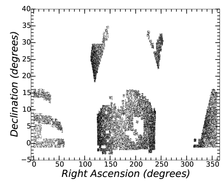
Figure 1.— The footprint of the UKIDSS LAS publicly available in DR8 (Ukidss, 2012) in right ascension and declination. UKIDSS LAS DR8 spans 2,400 deg² and contains over 69 million sources.

We corrected the $JHK$ magnitudes of all sources for reddening using the extinction maps of Schlegel et al. (1998), with the updated coefficients from Schlafly & Finkbeiner (2011). The reddening in our final sample was small, with a median $E(B-V)=0.048$ and a standard deviation of $\sigma_{E(B-V)}=0.043$. The maximum reddening in the sample was $E(B-V)=0.41$, below the limit of $E(B-V)=0.55$ set by Majewski et al. (2003).

2.2. Sloan Digital Sky Survey

The SDSS (York et al., 2000) was an optical photometric and spectroscopic survey of 14,555 deg.² (Ahn et al., 2013) conducted with the 2.5m telescope at the Apache Point Observatory (Gunn et al., 2006). The bulk of the survey was photometric, surveying the sky using a drift-scan technique. The camera contained 5 camera columns, each corresponding to one filter in the $ugriz$ system. With an exposure time of 53.9 seconds, the main survey achieved a faint limit of $r\sim$ 22, with typical systematic photometric errors of $\sim$ 0.02 mag for point sources (Ivezić et al., 2007). This was empirically verified using repeat scans of a 300 sq. deg. area near $\delta=0$, the so-called “Stripe 82”, which was imaged multiple times over the course of the survey (i.e., Becker et al., 2011).

When the skies above Apache Point were not photometric, the SDSS operated in spectroscopic mode. The spectrograph contained two cameras which simultaneously obtained $R\sim 1,800$ spectra for 640 objects through fiber optic cables (Uomoto et al., 1999). The typical exposure time was $\sim$ 45 minutes, resulting in many observations with S/N $>15$. As part of the Legacy and SEGUE surveys, stars were selected for spectroscopic followup by targeting algorithms designed to retrieve specific types of stars, such as cataclysmic variables (Szkody et al., 2002), brown dwarfs (Schmidt et al., 2010), K giants (Helmi et al., 2003) and a host of $\sim$15 other types of stars (Yanny et al., 2009b). Over 3 million unique optical spectra are publicly available in the latest data release (Ahn et al., 2013), including more than 600,000 stellar spectra. Recently, the Apache Point Observatory Galactic Evolution Experiment (APOGEE, Zasowski et al., 2013) obtained and published $\sim$ 60,000 NIR spectra of red giant stars, although these stars are much brighter than the ones presented here ($H\lesssim 12$).

The SDSS also delivered exquisite astrometry, with an internal precision of 25 mas and an absolute accuracy of 45 mas in each coordinate direction (Pier et al., 2003). A proper motion catalog was derived by comparing SDSS observations to the USNO-B catalog (Monet et al., 2003), with a typical baseline of 50 years. The resulting catalog (Munn et al., 2004) contains over 205 million objects with a median uncertainty of 2 mas yr^-1. These proper motions have been used to study a number of stellar populations, including nearby M dwarfs and subdwarfs (Bochanski et al., 2007a, 2013; Lépine & Scholz, 2008).

3. M Giant Candidate Selection

To identify the stars most likely to be M giants, we incorporate UKIDSS and SDSS photometry into our targeting algorithm. We also use proper motion estimates to cull out nearby M dwarfs. The process is explained below and summarized in Table 1.

3.1. Near-Infrared Color Cuts

The UKIDSS LAS DR8 catalog contains 69,656,410 sources, down to a faint limit of $K\sim 18.2$, covering $\sim 2,400$ sq. deg. We implemented a SQL query on the UKIDSS public database designed to only include high-quality detections of point sources (at the expense of completeness), yielding 6,969,163 objects. Our SQL query is available in Appendix A. From the catalog of point sources, we selected M giant candidates using the following NIR color-color cuts:

$$(J-K)_{\rm o}>1.02$$ (1)

$$(J-H)_{\rm o}<0.561\times(J-K)_{\rm o}+0.46$$ (2)

$$(J-H)_{\rm o}>0.561\times(J-K)_{\rm o}+0.185$$ (3)

This color selection was adapted from those of Majewski et al. (2003) and Sharma et al. (2010), but shifted slightly redward (in both $J-H$ and $J-K$), to reduce contamination from foreground M dwarfs. The most significant difference between our own selection and previous studies is contained in Eqn. 1. The M dwarf and M giant sequence begin to diverge in $JHK$ colors near $J-K\sim$ 0.85, with larger separation at redder colors (Lee, 1970; Glass, 1975; Mould, 1976; Bessell & Brett, 1988). By extending our color cuts redward, we maximize the separation from the locus of M dwarfs, minimizing the contamination of our M giant sample. Our NIR color selection is shown in Figure 2. This color selection is most sensitive to M giants with $[Fe/H]>-0.5$ (Dotter et al., 2008).

Since the number of M dwarfs is much larger than the number of M giants in the Galaxy, we estimated our contamination rate by comparing the number of M dwarfs expected to scatter into our selection box as a function of signal–to–noise (S/N) and color. In order to facilitate this computation, we computed the expected scatter as a function of $c_{1}$ color, which is a linear combination of $J-H,H-K$ colors defined as:

$$c_{1}=(J-H)-(0.561*(J-K))$$ (4)

This color effectively collapses the NIR colors along the slope of NIR giant selection box shown in Figure 2. M giants candidates have red $c_{1}$ colors, while M dwarfs and brown dwarfs have bluer $c_{1}$ colors. In steps of S/N = 5 from 5 to 100, we fit the low-mass stellar locus with a Gaussian, then computed the expected number of low–mass stars scattered into the M giant NIR selection box. The contamination level dropped quickly with rising S/N as: 1) The number of M dwarfs decreased and; 2) the separation between the M dwarf and M giant loci increased. We also calculated the expected contamination while adopting the Majewski et al. (2003) and Sharma et al. (2010) NIR color cuts. These previous studies were subject to greater M dwarf contamination due to their bluer $JHK$ color cuts. Our adopted cuts emphasize purity over completeness, avoiding the bluer $JHK$ color regions which do include M giants (Majewski et al., 2003, 2004) but are dominated by M dwarf contamination. After this experimentation, we implemented a S/N $=$ 15 for imaging in $JHK$, which translates to faint limits of $J,H,K=(18.47,17.66,17.05)$. At this fiducial S/N, we expect $\sim 25\%$ contamination from M dwarfs. However, the fraction of M dwarfs contaminating our final sample is larger, as detailed in Section 5.1.3. This cut resulted in 1,649 M giant candidates with NIR photometry.

3.2. Optical Color Cuts

Using the SDSS casjobs interface (O’Mullane et al., 2005), we cross-matched our list of M giant candidates against the SDSS DR10 PhotoPrimary catalog. Of the 1,649 NIR selected objects, 1,638 matched objects in SDSS within 30^′′. Although we permitted a large matching radius, the majority of stars (99.1%) had matches within 1^′′, with only 9 sources outside this radius. All of these distant matches were removed with proper motion cuts. We obtained $ugriz$ psf photometry, flags, and uncertainties for each object, as well as any available proper motions and spectroscopy. Of the matched UKIDSS-SDSS observations that passed our visual vetting (see Section 3.3), 98 were removed for having bad photometry in SDSS (clean = 0) or being morphologically identified as a galaxy (type = 3).

3.3. Visual vetting

During the course of our investigation, we learned of issues present in a fraction of the stacked $J$ band frames that result in $J$ magnitudes that are systematically faint by $\sim$0.14 mag (S. Warren, private communication, 2012). Unfortunately, no flags in the catalog alert the user to this anomaly. Such dimmed $J$ magnitudes make the $J-H$ and $J-K$ colors of affected stars artificially redder. Stars on flawed frames can be tossed out via visual inspection: the artifact is manifested as pixel-sized “holes” in the $J$ band imaging, equally spaced by a few pixels. These systematic errors affect entire $J$-band frames, with every star on a bad frame being dimmed. An example of a good and bad $J$ band image is shown in Figure 3. To achieve the highest fidelity, we visually inspected each matched SDSS-UKIDSS M giant candidate. Of the 1,638 matches to SDSS photometry, 992 were obtained with clean $J$-band frames. The remaining candidates were removed from our sample.

Table 1Summary of Target Selection

Dataset	Description	Stars Remaining
UKIDSS	Total UKIDSS DR8 LAS Footprint	69,656,410
UKIDSS	High quality imaging	6,969,163
UKIDSS	M Giant Color-Cuts, S/N = 15	1,649
UKIDSS $+$ SDSS	NIR $+$ Optical Match	1,638
UKIDSS $+$ SDSS	Visual Inspection	992
UKIDSS $+$ SDSS	Optical Color Cuts	464
UKIDSS $+$ SDSS	USNO-B-SDSS Proper Motions	409
UKIDSS $+$ SDSS	SDSS-UKIDSS Proper Motions	404

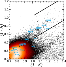
Figure 2.— The $J-H,J-K$ (Vega) color-color diagram for point sources in UKIDSS. Overplotted is our NIR color selection described in Equation 1 and the colors of M giants and dwarfs synthesized from the Pickles spectral library (light blue points, Pickles, 1998). Our NIR color selection is shifted to slightly redder $J-H,J-K$ colors than that of Majewski et al. (2003) and Sharma et al. (2010). This was done to reduce contamination of bluer, nearby M dwarfs, which dominate the stellar locus at bluer colors. This may reject some early–type giants, but should significantly reduce dwarf contamination.

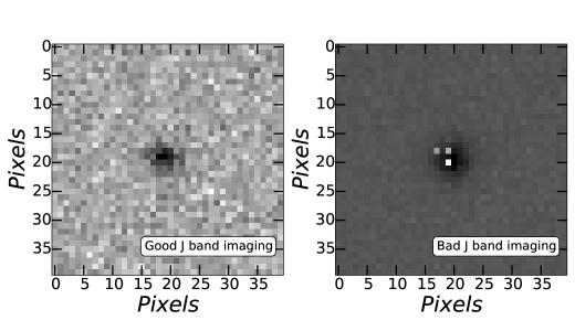
Figure 3.— An example of “bad” imaging in UKIDSS. The cutout on the left is a star that passed our visual verification, while the star on the right contained faulty $J$–band imaging and was rejected. Images were readily identified by “holes” offset by a few pixels, typically near bright sources. This effect removed 646 M giant candidates from our study.

3.4. Removing QSO Contamination

While the surface density of QSOs is small, they have NIR colors similar to M giants. Fortunately, NIR and optical colors can discriminate between the two classes. Peth et al. (2011) demonstrated that stars and QSOs separate in $g-i,i-K$ color-color space, as shown in Figure 4. We require our M giant candidates to satisfy:

$$g-i>0.932\times(i-K)-0.872$$ (5)

In the current sample, this cut removes nearly half of NIR selected candidates, with 466 M giant candidates remaining (and 428 removed). Finally, we enforced red optical colors, by requiring $g-r>0.5$ for all candidates, removing two objects from the catalog.

Since nearly half of our sample is removed with this cut, we initially suspected QSO contamination may have affected previous M giant studies. We investigated the effect of QSO contamination on catalogs of 2MASS–selected M giants (i.e., Majewski et al., 2003; Sharma et al., 2010). In Figure 5, we plot the apparent $K$ distribution of stars and stars and quasars, as defined by Equation 5. As seen in Figure 5, QSO contamination becomes important after $K\sim 14.5$, which is just beyond the faint limit of 2MASS ($K=14.3$). Although there are few UKIDSS sources bright enough to robustly test the possible impact of QSO contamination on 2MASS studies, our sample implies that previous studies would not have been significantly influenced by the presence of QSOs.

Our cut to remove QSOs was tested during an initial observing run for this project. We obtained Gemini GNIRS spectra (described in Section 4.2) of 14 M giant candidates selected with an old target selection algorithm that did not include proper motion or optical colors. Of the 14 targets, eight had $giK$ colors that would have been flagged as QSOs by Eqn. 5. All eight were spectroscopically confirmed as $z\sim 1.2$ QSOs, suggesting this cut is very effective at removing these contaminants.

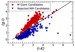
Figure 4.— The NIR-optical $g-i,i-K$ color-color selection used to remove QSOs (blue filled triangles) from our M giant candidates (red filled circles). Note that the QSOs have bluer $g-i$ colors at the same $i-K$. The combination of optical and NIR colors are essential for removing QSOs from the sample, which may have caused minor contamination in previous studies (i.e., Majewski et al., 2003; Sharma et al., 2010).

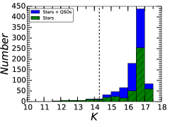
Figure 5.— The $K$ magnitude distributions of stars (hatched green histogram) and all objects (QSOS and stars; solid purple histogram) in our sample. Note that QSOs become more important at fainter magnitudes, well beyond the faint limit of 2MASS ($K=14.3$). This suggests that QSO contamination was not significant for previous studies that relied solely on photometric identification of M giants (i.e., Majewski et al., 2003; Sharma et al., 2010).

3.5. Proper Motion Cuts

M giants at halo distances should exhibit no discernible proper motion. Thus, we removed any stars with significant proper motions using the two following methods. The first used the proper motions measured between the SDSS and USNO-B catalog (Munn et al., 2004; Monet et al., 2003), which was based on observations mainly from the POSS survey (Minkowski & Abell, 1963). Proper motions, when available, were obtained from the ProperMotions table in SDSS DR10. With a typical baseline of 50 years, the precision of proper motion estimates was $\sim 2$ mas yr^-1. We used several cuts on precision and error flags to ensure high quality proper motions. These are described in detail in our previous investigations (i.e., Dhital et al., 2010; Bochanski et al., 2011; West et al., 2011). Any star that exhibited a proper motion larger than 2.5$\times$ the uncertainty in either right ascension or declination was flagged as moving. This cut removed 55 stars from our sample.

Since the Munn et al. (2004) proper motions are based on POSS observations, they lack sensitivity to faint red objects. We addressed this by computing proper motions using SDSS as the first epoch and UKIDSS as the second epoch. The astrometric positions are reported by the SDSS pipeline with an internal precision of 25 mas and an absolute accuracy of 45 mas in each coordinate direction (Pier et al., 2003). The UKIDSS astrometric precision ranges from 50-100 mas, depending on Galactic latitude (Lawrence et al., 2007; Scholz, 2010). We computed proper motions for each star using the UKIDSS and SDSS positions, and compared them to the Munn et al. (2004) proper motions as a function of temporal baseline (Figure 6). After $\sim 6$ years, the proper motions agree at a level of $\sim 40$ mas yr^-1. Any stars with a motion greater than 40 mas yr^-1 (in either coordinate) with a baseline of 6 years or greater were excluded from our sample, with 5 stars being removed.

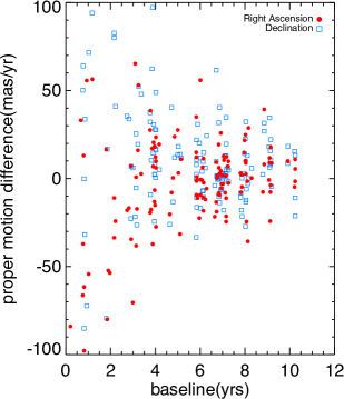
Figure 6.— The difference in proper motion as measured by Munn et al. (2004) and our SDSS-UKIDSS proper motions as a function of SDSS-UKIDSS temporal baseline. Proper motion differences in right ascension (filled red circles) and declination (open blue squares) follow similar distributions, with better agreement for longer baselines. The standard deviation in proper motion difference for baselines greater than six years is $\sim$ 40 mas yr^-1, which we adopt as our precision limit for SDSS-UKIDSS proper motions. Stars with motions greater than 40 mas yr^-1 in either direction, and with baselines greater than 6 years, were expunged from the sample. This removed five stars from our sample.

The GNIRS spectra were also useful for testing the effectiveness of our proper motion cuts. Of the six stars observed with GNIRS, two were flagged as moving, while four were not. All were spectroscopically confirmed as low–mass dwarfs, suggesting an efficiency of $\sim 30\%$. After the NIR, optical and proper motion cuts, 404 stars remained in our sample. These stars are listed in Table 2 and their NIR color–magnitude diagram is shown in Figure 7. Our initial spectroscopic followup is detailed in the following section.

Table 2M Giant Candidates

Name	RA	Dec	$u$	$\sigma_{u}$	$g$	$\sigma_{g}$	$r$	$\sigma_{r}$	$i$	$\sigma_{i}$	$z$	$\sigma_{z}$	$J$	$\sigma_{J}$	$H$	$\sigma_{H}$	$K$	$\sigma_{K}$
ULAS J000216.74+115533.0	0.56976	11.92584	25.32	0.67	24.93	0.49	22.36	0.16	20.33	0.04	19.17	0.06	17.46	0.03	16.73	0.03	16.44	0.04
ULAS J001228.63+003049.8	3.11930	0.51384	23.52	0.79	21.77	0.06	20.31	0.03	19.03	0.02	18.30	0.03	17.16	0.02	16.40	0.03	16.10	0.03
ULAS J001507.92+070058.8	3.78301	7.01634	25.37	0.76	23.05	0.22	21.58	0.08	19.97	0.03	19.04	0.05	17.70	0.05	16.90	0.05	16.66	0.06
ULAS J001535.72+015549.6	3.89882	1.93045	25.03	1.02	21.16	0.04	19.80	0.03	19.12	0.02	18.74	0.04	17.73	0.06	17.00	0.04	16.70	0.05
ULAS J001701.41+081837.4	4.25585	8.31038	22.64	0.59	22.59	0.22	21.73	0.12	20.11	0.04	19.09	0.07	17.74	0.04	16.98	0.05	16.69	0.05
ULAS J001827.65+142946.6	4.61523	14.49629	22.73	0.56	20.02	0.03	18.69	0.02	17.93	0.02	17.45	0.02	16.49	0.01	15.67	0.02	15.43	0.02
ULAS J002219.76+073542.6	5.58232	7.59516	23.09	0.38	21.80	0.06	20.55	0.03	19.62	0.02	19.15	0.04	18.11	0.08	17.34	0.06	17.02	0.07
ULAS J002226.36+071711.8	5.60981	7.28662	24.39	0.63	23.49	0.21	21.94	0.07	20.24	0.03	19.41	0.05	17.89	0.05	17.16	0.05	16.87	0.06
ULAS J002548.91+150745.0	6.45381	15.12918	23.71	0.75	23.41	0.36	21.37	1.63	19.95	0.77	19.21	0.19	17.74	0.06	16.87	0.05	16.65	0.07
ULAS J003048.68-005859.0	7.70284	-0.98305	23.15	0.45	20.56	0.03	19.33	0.02	18.77	0.02	18.50	0.03	17.50	0.05	16.72	0.04	16.46	0.06
ULAS J003105.14+144525.5	7.77140	14.75709	24.86	0.74	22.89	0.17	21.48	0.07	20.07	0.03	19.26	0.06	17.95	0.06	17.15	0.06	16.93	0.08
ULAS J003448.36+142924.6	8.70150	14.49016	23.29	0.56	21.93	0.08	20.52	0.04	19.65	0.03	19.16	0.05	18.12	0.07	17.31	0.08	17.01	0.08
ULAS J003501.38+150324.4	8.75574	15.05677	23.82	0.90	20.87	0.04	19.53	0.02	18.82	0.02	18.47	0.04	17.40	0.03	16.60	0.04	16.38	0.05
ULAS J004216.12+084509.9	10.56717	8.75276	22.95	0.69	23.91	0.74	21.94	0.13	20.32	0.05	19.45	0.09	17.95	0.04	17.17	0.06	16.91	0.07
ULAS J004255.06+065205.1	10.72943	6.86808	23.29	0.75	21.44	0.06	20.02	0.03	19.36	0.03	18.86	0.05	17.91	0.05	17.11	0.05	16.85	0.07
ULAS J004505.03+141010.8	11.27094	14.16967	22.65	0.44	22.61	0.19	21.35	0.07	20.01	0.03	19.30	0.06	18.01	0.05	17.26	0.06	16.94	0.07
ULAS J004823.61+135332.6	12.09837	13.89238	25.42	0.84	24.21	0.81	21.74	0.15	20.28	0.05	19.48	0.08	18.01	0.06	17.28	0.07	16.98	0.08
ULAS J005100.87+073514.1	12.75361	7.58724	24.35	0.92	24.01	0.37	22.00	0.09	20.18	0.04	19.24	0.06	17.08	0.02	15.82	0.02	15.22	0.02
ULAS J005235.98+141555.4	13.14991	14.26539	24.46	0.85	22.41	0.13	21.00	0.06	19.86	0.03	19.22	0.05	18.01	0.05	17.23	0.06	16.96	0.07
ULAS J005608.18+052041.9	14.03406	5.34497	23.49	0.77	23.81	0.37	22.10	0.13	20.47	0.04	19.31	0.07	17.93	0.05	17.14	0.04	16.83	0.06
ULAS J005618.98+084641.0	14.07907	8.77805	22.62	0.52	21.81	0.10	20.19	0.04	19.47	0.03	19.06	0.06	18.00	0.06	17.09	0.04	16.88	0.06
ULAS J005859.41+134710.6	14.74753	13.78627	23.58	0.70	23.31	0.30	21.69	0.08	20.18	0.03	19.32	0.06	18.09	0.06	17.35	0.06	17.03	0.08
ULAS J005908.48+085015.2	14.78533	8.83756	23.24	0.70	21.25	0.05	19.87	0.03	19.29	0.04	18.88	0.05	18.02	0.06	17.12	0.04	16.85	0.06
ULAS J010008.14+143019.1	15.03390	14.50529	24.83	0.70	21.71	0.07	20.34	0.03	19.49	0.02	18.98	0.05	17.82	0.05	17.09	0.06	16.79	0.06
ULAS J010133.53+160158.7	15.38973	16.03297	24.49	1.08	22.36	0.23	20.24	0.07	19.54	0.06	19.25	0.12	18.14	0.07	17.35	0.06	17.01	0.07
ULAS J010418.99+001356.7	16.07913	0.23243	22.81	0.34	21.29	0.04	19.97	0.02	19.30	0.02	18.89	0.04	17.90	0.04	17.07	0.05	16.82	0.06
ULAS J011215.23+060439.4	18.06347	6.07762	24.98	0.73	22.03	0.13	20.68	0.04	19.34	0.02	18.60	0.03	17.38	0.03	16.59	0.03	16.34	0.03
ULAS J011531.60+000344.9	18.88165	0.06249	25.57	0.45	23.09	0.15	21.71	0.06	20.25	0.03	19.42	0.06	18.00	0.05	17.20	0.06	16.84	0.07
ULAS J011641.58+065101.6	19.17325	6.85044	23.34	0.74	24.15	0.56	22.11	0.17	20.36	0.05	19.36	0.07	18.13	0.06	17.25	0.05	17.01	0.06
ULAS J011954.61+133849.6	19.97753	13.64711	25.46	0.60	22.25	0.11	20.72	0.04	19.76	0.03	19.13	0.05	18.19	0.06	17.27	0.06	17.02	0.07
ULAS J012226.41+152428.7	20.61004	15.40798	24.61	0.91	21.04	0.04	19.78	0.03	19.12	0.02	18.67	0.04	17.60	0.04	16.78	0.02	16.55	0.04
ULAS J012254.91+061151.2	20.72879	6.19757	24.59	0.94	21.46	0.06	20.10	0.02	19.35	0.02	18.96	0.04	17.87	0.04	17.05	0.04	16.84	0.05
ULAS J012453.59-004120.4	21.22329	-0.68899	22.58	0.26	21.59	0.06	20.14	0.04	19.29	0.02	18.90	0.03	17.84	0.06	17.09	0.04	16.81	0.06
ULAS J012754.13+064807.5	21.97554	6.80207	22.62	0.27	23.56	0.22	22.15	0.09	20.41	0.04	19.29	0.05	17.93	0.04	17.17	0.05	16.85	0.05

Note. — This is an abbreviated list.

4. Initial Spectroscopic Campaign Results

In this section, we describe our initial spectroscopic campaign, which included observations using five different spectrographs. The results from our spectroscopic follow-up follows in Section 5.

4.1. IRTF–Spex

We obtained the bulk of our NIR observations with SpeX at the NASA Infrared Telescope Facility (IRTF). We observed a total of 13 M giant candidates during 3 nights. The SpeX observations span 0.8 to 2.5 µm, covering the $JHK$ bandpasses. We obtained 11 spectra in SXD mode with the 0^′′.8 slit, and two spectra in prism mode with the 0^′′.5 slit, resulting in spectral resolutions of $R\sim$ 750 and 150, respectively. The data were reduced using the IDL package Spextool (Cushing et al., 2004). This program flat fields and wavelength calibrates each spectrum before performing an optimal extraction. Telluric correction and flux calibration was performed by comparing A0V stars observed near each science target to spectra of Vega in the xtellcor package. The results of the IRTF observing runs are given in Table 3.

4.2. Gemini Near–Infrared Spectrograph

We obtained 14 near–infrared (NIR) spectra of M giant candidates selected with a preliminary targeting algorithm that did not including proper motions or optical color cuts with the Gemini NIR spectrograph (GNIRS; Elias et al., 2006) at the Gemini Observatory in Mauna Kea, Hawaii. Only four of the spectra pass our final criteria and are presented in Table 3. These early observations were important for testing our quasar and proper motion selection criteria. Of the 14 observed candidates, eight were photometrically eliminated as QSOs in our final target selection algorithm and were spectroscopically confirmed as QSOS. The remaining six candidates were all identified as M dwarfs, with two being flagged as moving, while the other four met all of our criteria. These four were spectroscopically classified as M dwarfs. As discussed in Section 5.1.3, this suggests that proper motion selection has an efficiency of $\lesssim 30\%$.

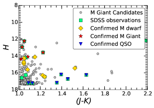
Figure 7.— The $J-K,H$ color–magnitude diagram for our final M giant candidate sample. Spectroscopically confirmed giants are shown with red filled stars, M dwarfs are shown with yellow filled diamonds, and spectroscopically identified QSOs are shown with blue filled triangles. Most of our candidates have 1.0 $<(J-K)_{o}<$ 1.2, and our confirmed M giants have $H$ brighter than 15. We expect more distant M giants will be found as we followup these targets with larger telescopes.

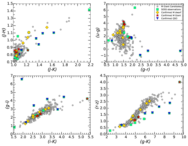
Figure 8.— Various color-color diagrams for the M giant candidate sample, along with our spectroscopic observations. The M giant sample (grey filled squares) has had preliminary spectroscopic followup with SDSS (green filled squares), along with our own observations, yielding QSOs (blue filled triangles), M dwarfs (yellow filled diamonds) and M giants (red filled stars). It is clear that most QSOs are outliers on the stellar locus, with blue $J-K,g-r$ and $g-K$ colors. In particular, the $r-z,g-K$ color-color diagram (lower right panel) demonstrates a clear separation from the stellar locus. The $u-g,g-r$ color-color diagram suggests that M giants are found at redder $u-g$ colors (see also Yanny et al., 2009b). There is also suggestive clumping of the confirmed M giants in $r-z,g-K$ color-color space, and this will be further explored in follow-up studies.

The spectra were cross–dispersed and imaged with the short wavelength camera. The spectra were obtained with the 32 lines per mm grating and the 0.^′′30 slit. Each spectrum spans the NIR wavelength regime, from 0.9 to 2.5 µm with a resolution $R\sim 1700$. The spectra were reduced using the gnirs package in the Gemini IRAF computing environment. The pipeline corrects for non–linearity, flat fields each image, and performs sky–subtraction from each AB nod. The spectra are wavelength calibrated from Argon lamp spectra, and each order is traced and corrected for curvature before extraction. For telluric correction, we employed the general version of the xtellcor routine first designed for the SpeX spectrograph at the NASA Infrared Telescope Facility (Cushing et al., 2004). The telluric corrections are computed by comparing the spectrum of an A0V star obtained close to the science target to a spectrum of Vega reddened using the $B-V$ color of the A star. The two spectra are shifted to the same velocity and the telluric correction and flux calibration is computed.

4.3. SOAR – Goodman Spectrograph

We obtained optical spectra of three M giant candidates with the Goodman High Throughput Spectrograph at the 4.1m Southern Astrophysical Research (SOAR) telescope at Cerro Pachón, Chile. These were also targeted with an early version of our selection algorithm. The targets obtained with SOAR are not included in our final catalog, so this spectroscopic campaign is not included in Table 3. The single order spectra were obtained with the 1^′′.03 slit and the 930 lines per mm VPH grating centered at 8100 Å. This setup spans 7250 to 8950 Å with a resolution of $R\sim 4470$. The images were reduced using IRAF routines. Each spectrum was flat-fielded, wavelength calibrated using CuNeAr arc lamp spectra, and extracted. Flux standards were obtained each night for calibration.

4.4. FIRE

We obtained a NIR spectrum of one M giant candidate using the Folded Port Infrared Echellette Spectrograph on the Baade Magellan Telescope (FIRE; Simcoe et al., 2013). FIRE is a single-object spectrograph capable of two modes: a single order, low-resolution prism mode, and a cross–dispersed echellette, covering 0.8–2.5 µm ($JHK$) over 21 orders. On May 15, 2013, we obtained a 1505s exposure of the M giant candidate. The 0${}^{\prime\prime}.6$ slit was used and aligned with the parallactic angle and the airmass was $1.18$. An A0V star, HD123233, was obtained for flux calibration and telluric corrections. The images were reduced using the FIRE reduction software package, FIREHOSE, which is based on the MASE pipeline (Bochanski et al., 2009) for the MagE spectrograph (Marshall et al., 2008). FIREHOSE is used to flat field images, find and trace orders, compute wavelength calibrations from OH telluric emission lines, and extract and combine each spectrum. A modified version of xtellcor was used to correct for telluric absorption. Our FIRE observation is listed in Table 3.

4.5. SDSS

In addition to the spectra obtained during our initial observational campaign, 15 M giant candidates had existing SDSS spectra in DR10 (Ahn et al., 2013). SDSS provides $R\sim 1,800$ resolution optical spectra, covering 3800 to 9200 Å. Each SDSS spectrum contains a variety of ancillary data, including redshift (or radial velocity for stars), spectral type, and targeting information. While the pipeline spectroscopic identification is usually reliable, we incorporated detailed visual inspection of all M star spectra. Of the 15 SDSS spectra, six were classified as QSOs, two were classified as M dwarfs, two as carbon stars, one as an F dwarf, and four M giants by the standard SDSS pipeline (Stoughton et al., 2002). Color–color diagrams for the objects with SDSS spectra compared to the rest of our candidates are shown in Figure 8. The F dwarf is much bluer in $g-i,i-K$ than the majority of the sample. The QSOs are also outliers when compared to the locus of candidates. Carbon stars and M dwarfs are more difficult to distinguish in the $ugrizJHK$ color space, but the $u-g,g-r$ color-color diagram may be useful in discriminating between M giants and other red stars, as previously shown by Yanny et al. (2009a, b). The results of the SDSS spectroscopy are listed in Table 3.

Table 3M Giant Candidates with Spectroscopic Followup

Name	RA	Dec	Instrument	Sp. Type	$RV$ (km s-1)	$d$ (kpc)	Notes
ULAS J074048.14+261900.2	115.20059	26.31671	Spex	M giant	$45.0\pm 20.0$	61
ULAS J075554.26+273130.9	118.97609	27.52525	SDSS, Spex	M giant	$15.9\pm 10.2$	52
ULAS J132441.60-004452.4	201.17332	-0.74790	SDSS	M giant	$-8.6\pm 9.7$	22
ULAS J145254.25-004826.0	223.22605	-0.80723	SDSS	M giant	$39.3\pm 2.5$	28
ULAS J151430.44+093722.5	228.62683	9.62293	SDSS	M giant	$24.1\pm 8.4$	92
ULAS J013510.10+004328.8	23.79209	0.72466	SDSS	QSO	$z=1.38$	$\cdots$
ULAS J020549.70+010856.5	31.45709	1.14904	SDSS	F star	$-45\pm 12$	59	F star with anomalous red colors
ULAS J021121.56-003808.5	32.83984	-0.63568	GNIRS	M dwarf	$\cdots$	68
ULAS J032746.74-000708.8	51.94477	-0.11911	GNIRS	M dwarf	$\cdots$	122
ULAS J033217.09+002204.0	53.07120	0.36778	SDSS	QSO	$z=4.83$	312
ULAS J073229.88+250554.0	113.12449	25.09833	GNIRS	M dwarf	$\cdots$	75
ULAS J073248.36+272115.5	113.20151	27.35430	GNIRS	M dwarf	$\cdots$	322
ULAS J074030.06+275224.0	115.12525	27.87333	Spex	M dwarf	$\cdots$	56	SXD mode
ULAS J083058.67+013448.7	127.74446	1.58019	Spex	$\cdots$	$\cdots$	82	SXD, poor S/N
ULAS J083510.60+022253.4	128.79419	2.38150	Spex	$\cdots$	$\cdots$	92	SXD, inconclusive
ULAS J095021.27+022653.2	147.58862	2.44810	Spex	$\cdots$	$\cdots$	112	SXD, inconclusive
ULAS J100821.40+121348.6	152.08916	12.23016	Spex	$\cdots$	$\cdots$	97	Prism, inconclusive
ULAS J102403.07+105121.6	156.01278	10.85600	Spex	$\cdots$	$\cdots$	167	SXD, inconclusive
ULAS J111523.25+082918.5	168.84687	8.48848	SDSS	QSO	$z=4.77$	265
ULAS J113931.61+050231.0	174.88172	5.04195	SDSS	$\cdots$	$-43\pm 16$	147	likely an M dwarf
ULAS J130619.39+023659.1	196.58080	2.61640	SDSS	QSO	$z=4.80$	1019
ULAS J132856.67+085713.8	202.23615	8.95383	SDSS	QSO	$z=4.14$	637
ULAS J135418.66-011430.7	208.57775	-1.24187	Spex	$\cdots$	$\cdots$	94	SXD, inconclusive
ULAS J141939.74+101803.3	214.91560	10.30092	Spex	$\cdots$	$\cdots$	171	SXD, inconclusive
ULAS J142526.11+082718.7	216.35877	8.45518	SDSS	QSO	$z=4.95$	1111
ULAS J142603.74+090326.4	216.51559	9.05735	SpeX	$\cdots$	$\cdots$	96	SXD, inconclusive
ULAS J144239.85+094124.3	220.66606	9.69008	Spex	M dwarf	$\cdots$	82	SXD mode
ULAS J144631.08-005500.3	221.62949	-0.91674	SDSS	Carbon star	$79\pm 4$	$\cdots$	Estimated distance $>$ 5000 kpc
ULAS J145112.50+020744.3	222.80206	2.12897	Spex, FIRE	M dwarf	$\cdots$	546	Observed with prism and SXD mode
ULAS J150738.22+104610.6	226.90924	10.76960	SDSS	Carbon star	$113\pm 6$	151
ULAS J221714.27+003346.5	334.30948	0.56292	SDSS	M dwarf	$59\pm 24$	331

5. Analysis

5.1. Spectroscopic Results

5.1.1 Preliminary Classification

We obtained spectra of 31 M giant candidates using our current algorithm, along with Gemini and SOAR spectra of 13 targets chosen with an earlier version of the pipeline. Each spectrum was manually inspected. We did not attempt to classify spectra with low S/N, removing nine stars from our sample. QSOs were easily identified by their non-stellar SEDs and removed from the sample. For the SDSS spectra, the pipeline produces a spectral type estimate by comparison to template spectra. We relied on these spectral types for the identification of non-M stars. This included one F star with red photometric colors and two carbon stars. Thirteen M star spectra remained after these cuts, and our dwarf/giant discrimination routine is discussed below.

5.1.2 M Giant / Dwarf Separation

For the NIR spectra obtained with Gemini, FIRE and Spex, we compared the spectra to M star spectra available in the IRTF spectral library (Cushing et al., 2005; Rayner et al., 2009). The IRTF library contains 86 dwarf and giant spectra, covering 0.8-5.0 µm with a resolution of $R\sim 2,000$. Each science target and template were normalized to a common scale, and the SEDs were compared. We examined both the overall agreement in $JHK$ between the science target and template, and the detailed comparison centered on luminosity–sensitive features in the NIR. Specifically, the Na doublet near 0.82 µm, the Ca triplet near 0.86µm, the Wing-Ford FeH band at 0.99 µm, neutral Na at 1.14 µm, and the CO bandheads in $H$ and $K$ were all examined as they are reliable dwarf$/$giant discriminators (Cushing et al., 2005). In Figure 9, we compare dwarf and giant spectra from our study. The luminosity sensitivity of the Na I lines and CO bands are readily apparent (see also Figure 21 of Cushing et al., 2005). Usually, a given science spectrum would have spectral features similar to many dwarf or giant spectra, ensuring a consistent luminosity class identification. For the identified M dwarfs, the spectral subclass was usually known to $\pm$ 1 spectral subtype.

Optical identification of giants was achieved by comparing the optical spectra from SDSS and SOAR against the Bochanski et al. (2007b) M dwarf templates. These templates are high signal–to–noise averages of M dwarfs with SDSS spectroscopy. Since the Na I line at 8200 Å is very strong in dwarfs (and weak in giants), the presence (or lack) of significant absorption was used as luminosity indicator (Schlieder et al., 2012).

5.1.3 Contamination

While our photometric and proper motion cuts were designed to remove contaminants from the M giant candidates sample, low–mass dwarfs and QSOs, along with other less common contaminants crept into our spectroscopic targets. It is useful to compare the expected and actual purity of our final sample. Of the 992 M giants candidates that had clean SDSS and UKIDSS photometry, we estimated $\sim 25\%$ were actually low–mass dwarfs using the $c_{1}$ color distribution. Cutting against QSOs removed nearly half the sample, at a fidelity close to $100\%$, as evidenced by the GNIRS spectra. This effect actually increases the contamination due to M dwarfs in the final sample. The remaining candidates were expected to be comprised of nearly equal numbers of M dwarfs and M giants (50% contamination from M dwarfs), plus some unknown fraction of high–redshift ($z>4$) QSOs and other contaminants. The proper motion selection removed $\sim 30\%$ of the M dwarfs, but was not nearly as effective at the QSO cut. Our spectra followup of 22 M giant candidates with high S/N yielded five bona-fide M giants, along with eight M dwarfs and nine other contaminants. This suggests that the remaining 404 candidates have a purity of $\sim 20\%$, with contamination being due to both M dwarfs and more exotic contaminants (carbon stars, $z>4$ QSOs), in roughly equal numbers. We draw two conclusions from this initial survey. First, M dwarf contamination is significant within our sample, with M dwarfs outnumbering M giants by at least a factor of two (i.e., 66% contamination). This is somewhat larger than our expected fraction of $\sim 50\%$. Second, our initial study suggests that contamination from exotic contaminants is relatively important in this sample, but we note that these contaminants were exclusively observed by SDSS, which targetted QSOs explicitly. We expect that as our survey continues, the fraction of M dwarfs will increase relative to the number of exotic contaminants.

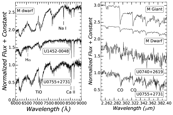
Figure 9.— Left Panel: Optical spectra of two of our M giant candidates, along with an M3 SDSS spectral template (Bochanski et al., 2007b). The main differences between the giants and dwarfs are seen in the differ morphology near the TiO bandheads and the lack of strong Na I absorption at $\sim 8200$ Å in the M giants. Right Panel: $K$ band spectra of two M giants from our study, as well as an M3 giant and M3 dwarf from the IRTF spectral library (Cushing et al., 2005). Giants possess significantly stronger CO bands than their dwarf counterparts.

5.1.4 Radial Velocities

Two of our spectroscopically confirmed M giants have radial velocities (RVs) measured with the SDSS spectroscopic pipeline (York et al., 2000; Stoughton et al., 2002). The radial velocity of ULAS  J074048.14+261900.2, which was observed only with Spex, was computed by cross–correlating it against Spex observations of ULAS J075554.26+273130.9, which was observed with Spex and SDSS, and assuming the SDSS-measured velocity for the template (Tonry & Davis, 1979). Due to the lower resolution of the Spex observations, the uncertainty on the RV for the third star is larger than the uncertainty for the SDSS RVs ($\sim 10$ km s^-1).

Radial velocities are reported in Table 3. We compared the positions, distances and velocities of these M giants to the model predictions of the Sgr stream (Law & Majewski, 2010). For each M giant, we computed the median velocity and distance predicted by the model for each wrap of the leading and trailing arms. We selected 25 of closest spatial matches for each wrap to compute the median model predictions. These predictions, along with our estimated distances, velocities and arm associations are shown in Table 4.

Table 4Confirmed M Giants in SGR

Name	RA	Dec	$V_{gsr}$	$V_{gsr,m}$	$d$	$d_{m}$	Arm
ULAS J074048.14+261900.2	115.20059	26.31671	227	146	61	39	$1^{st}$ Trailing
ULAS J075554.26+273130.9	118.97609	27.52525	190	151	52	39	$1^{st}$ Trailing
ULAS J132441.60-004452.4	201.17332	-0.74790	-99	-62	22	20	$1^{st}$ Trailing
ULAS J145254.25-004826.0	223.22605	-0.80723	-122	-109	28	23	$1^{st}$ Trailing
ULAS J151430.44+093722.5	228.62683	9.62292	-148	-164	92	55	$2^{nd}$ Trailing

5.2. Photometric Results

5.2.1 Galactic Distribution

Figure 10 shows the distribution of our M giant candidates in Galactic latitude and longitude. We compared the spatial distributions of the M giant candidates to those of two different samples: 1) a UKIDSS-selected M dwarf sample (point sources with bluer colors and S/N $=$15, see Figure 2) and 2) a sample composed of 50% M dwarfs and 50% QSOs, similar to our contaminants. If (a fraction of) the M giant candidates are true M giants then the spatial distribution of M giant candidates should be different than that of either comparison sample, with M dwarfs populating the Galactic thin and thick disks, and M giants distributed within the Galactic halo.

First, we generated each test sample to match the total number of M giant candidates. Next, we calculated a two–dimensional Kolmogorov–Smirnov test comparing the M giant candidates’ Galactic distribution to the contaminant distribution (Fasano & Franceschini, 1987). This test was repeated 10,000 times with a random sub-sample of contaminants for each test, recording the probability each time. For the contaminant sample composed only of M dwarfs, the median probability was 5 $\times 10^{-4}$, strongly suggesting that the M giant candidates and M dwarf samples were not drawn from the same 2D spatial distribution. We examined the cumulative distribution function for the 10,000 2D KS-test probabilities and found that 99.6% of all tests had probabilities of $<5\%$, further strengthening the suggestion that the M giants candidates and M dwarfs are not drawn from the same parent population. The contaminant sample composed of QSOs and M dwarfs had a similar probability, with 98.4% of all tests have a probability of $<5\%$. Since there is a lack of M giant candidates near ($\ell,b$) $\sim$ (50^∘,50^∘), we ran the test again, since this may artificially increase the difference between the M giant and contaminant distributions. We removed stars in this region and recomputed the above test. No difference between the cleaned samples were detected.

In Figure 10, we compare the average spatial density (in stars/deg²) of the M giant candidates (left panel), the average map of M dwarf contaminants, computed after 10,000 iterations (center panel) and the logarithm of the ratio of the two distributions (right panel). The red areas indicate an excess of M giant candidates compared to the average M dwarf spatial density, whereas blue indicates an excess of dwarf stars. Most of the M giant excess are near an absolute Galactic latitude of $\sim 50$, indicating that many of these stars are likely not distributed within the Milky Way’s disk.

5.2.2 Distances

Photometric parallax relations for M giants are plagued with uncertainty. Some recent studies have advocated using a single absolute magnitude (Yanny et al., 2009a; Palladino et al., 2012, i.e., $M_{r}\sim-2.3$), while other studies advocate simple linear relations (Sharma et al., 2010), with large $(\gtrsim 1$ mag) scatter in absolute magnitude (as compared to $\sim$ 0.2 mag for M dwarfs, Bochanski et al., 2010). The relations and assumed metallicities are described in Table 5 and were used to estimate distances to all of the M giant candidates in our sample. We adopted the Bovy et al. (2012) distance estimates as our fiducial distances. Briefly, the Bovy et al. (2012) distances computed by generating a probability distribution in $M_{H},(J-K)$. This probability distribution is computed using the Padova isochrones, an assumed metallicity, an initial mass function (IMF; Chabrier, 2003), and an assumed star formation history (SFH; either constant or exponentially declining). The number of stars as a function of $M_{H},J-K$ is computed, and the probability of a star with $M_{H}$ is computed for a given $J-K$. We used the peak of each $M_{H},J-K$ probability function to compute our distances. We refer the reader to Appendix A of Bovy et al. (2012) for a further description of this method. The benefits of this distance estimator is that it does not rely on a single color–magnitude relation, such as the Nikolaev & Weinberg (2000) or Yanny et al. (2009a) which assumed the color–magnitude relation of the LMC and M71, respectively. The histogram of distances for M giant candidates in our sample is shown in Figure 11.

To quantify the dependence of distance on the assumed parameters (metallicity and star formation rate), we varied these parameters and re-calculated the distance to each M giant candidate. We found similar results whether we assumed a constant or exponentially declining SFH. However, the assumed metallicity of the stellar population has a significant influence on the computed M giant distances, as shown as the different histograms in Figure 11. For the stars in our sample, the average distance migrates $\sim 100$ kpc outward for each step of $-0.5$ in metallicity. Given that only the oldest M giants can have low metallicities ($[Fe/H]\sim-1$), we expect that the majority of M giants in our sample are within 200-400 kpc. The structure seen in Figure 11 is due to two major factors: the distribution of stars in the halo and contamination from nearby M dwarfs. Given that the halo stellar density distribution decreases as $\sim d^{-3}$ (Jurić et al., 2008), while the volume increases by the same factor, we would naively expect a flat or falling distribution of distances. Thus, the peaks seen in Figure 11 are not inherent properties of the halo, and are likely the result of contamination.

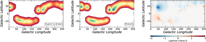
Figure 10.— Left Panel: The density of M giant candidates on the sky (stars / sq. deg.) estimated using a $k=12$ nearest neighbors algorithm from the astroml python package (VanderPlas et al., 2012). Center Panel: Same as above, but the median density of M dwarfs (from 10,000 random draws matching the M giant candidates in number). Right Panel: The logarithm of the ratio of the two panels. Note that most of the M giant excesses (shown as red) are far from the Galactic plane, suggesting these may be significant oven-densities.

Table 5Photometric Parallax Relations for M giants

Paper	Relation	Assumed $[Fe/H]$	Source
Nikolaev & Weinberg (2000)	$M_{K}=-5.5$	$\sim-0.7$	2MASS photometry of the LMC
Yanny et al. (2009a)	$M_{g}=-1.0,M_{r}\sim-2.3$	$\sim-0.8$	$ugriz$ photometry of M71 (An et al., 2008; Clem et al., 2008)
Sharma et al. (2010)	$M_{K}=3.26-9.42\times(J-K)$	$\gtrsim-1$	Isochrones and ages from $6-13$ Gyr
Palladino et al. (2012)	$M_{r}=0.8,M_{i}=-1.5,M_{z}=-3.5$	$\sim 0$	Pickles (1998) spectral templates
Bovy et al. (2012)	$P(M_{H}|J-K)$	Varies	Assumed SFH, IMF and isochrones

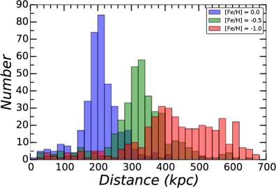
Figure 11.— The histogram of distances for M giant candidates in our sample. Distances were derived using the methods described in Bovy et al. (2012). The majority of the candidates have distances of 150-300 kpc, with very few stars being found at larger distances. The confirmed QSOs in our sample have been removed to make this figure, as their computed distances were $>1000$ kpc.

6. Discussion and Conclusions

Using a combination of NIR and optical photometry and spectroscopy from UKIDSS and SDSS, we have assembled a catalog of 404 M giant candidates. We have identified five M giants with distances from $\sim 20-90$ kpc, and are currently targeting fainter M giant candidates. These fainter stars, if truly M giants, lie at typical distances of $\sim$ 200 kpc (assuming $[Fe/H]$ = 0.0), more distant than any known Milky Way star. The photometric distance estimates for M giants are highly dependent on their assumed $[Fe/H]$, and increase by $\sim$50% for each 0.5 dex of decreasing $[Fe/H]$.

We found that optical-NIR cuts to eliminate QSOs and proper motion cuts to eliminate foreground M dwarfs were essential. Nearly half of the possible M giant candidates were removed when selecting against things with QSO–type colors. Prior studies that relied solely on NIR photometry to select M giants are only marginally contaminated by QSOs, but contamination becomes important at fainter ($K>14$) magnitudes. Early spectroscopic follow-up with Gemini/GNIRS and SOAR confirmed the importance of including both optical photometry and proper motions as a complement to NIR-selected M giants. In these early samples, objects with NIR$+$optical colors consistent with QSOs and with proper motions consistent with M dwarfs were spectroscopically confirmed to be such with an efficiency of 100%.

Our initial campaign to follow-up the 404 M giant candidates resulted in 22 candidates with sufficiently high quality spectra to make a robust classification. 5 of these 22 are M giants, which naively implies that $\sim$20% of our M giant candidates are true M giants. However, 15 of these 22 spectra are public SDSS spectra targeted because of their unusual colors, for example as indicative of QSOs (6 of the 15) or carbon stars (2 of the 15). The color distribution of these 15 SDSS targets is significantly different than the overall color distribution of our M giant candidates (Figure 8), so our M giant selection efficiency may be significantly different from 20%.

In the context of $\Lambda$-CDM cosmology, accretion plays an important role in the assembly and evolution of the Galactic halo. The archetypal accretion event contributing M giants to the Milky Way’s halo is the Sagittarius Dwarf Galaxy (Majewski et al., 2003). The Sgr dwarf contributed a significant fraction of the halo’s M giants, with nearly 75% of halo M giants (at distances $<$ 50 kpc) coming from the Sgr dwarf (Majewski et al., 2003). We can use our catalog to loosely constrain the number of Sgr-like accretions that could have built up the Galactic halo by comparing our number of M giant candidates with the expected number of M giants that a Sgr-like accretion would contribute. To do this, we estimate the number of M giants in Sgr by dividing the total luminosity of the system ($\sim 1\times 10^{7-8}L_{\odot}$; Niederste-Ostholt et al., 2010) by the typical luminosity of an M giant ($\sim 1\times 10^{3}L_{\odot}$; Dotter et al., 2008) and scaled by the fraction of luminosity produced by M giants. We employed a variety of metallicities ($Fe/H=0.0,-0.2,-0.5,-1.0$) and ages (3, 5, 10 Gyr) to compute the fraction of luminosity in M giants for that model. For a given cutoff in luminosity, this fraction ranged from 1-30%. Thus, given the uncertainties in the total luminosity of Sgr and the fraction of light being emitted by M giants, we expect 10-3000 M giants contributed for each Sgr-accretion event. Assuming an isotropic distribution of M giants on the sky, we expect $\sim 1-125$ M giants within our UKIDSS sample. If we naively interpret the 80$\%$ contamination rate of our initial spectroscopic sample, then we expect $\sim 80$ bona-fide M giants within our sample, which is consistent with the accretion of at least a single Sgr-like dwarf. As explained above, we are biased against the bluest M giants. We quantified this bias by calculating the fraction of Sgr giants missed by adopting our NIR color cuts. Using spectroscopically confirmed M giants (Majewski et al., 2004), we recover $\sim 30\%$ of M giants contained within Sgr. We note that many of the M giants presented in Majewski et al. (2004) are early-type M0-M2 giants. While this cut is necessary to avoid crippling M dwarf contamination, it suggests that the predicted number of M giants in our sample ($\sim 80$), and thus the predicted number of Sgr-type accretion events, is a lower limit for the outer halo. While all of the M giants presented in this work can be associated with Sgr, M giants found at larger distances ($d>100$ kpc) are less likely to be well–modeled as Sgr members (Law & Majewski, 2010). Other stellar tracers, such as blue horizontal branch stars, and RR Lyrae (Deason et al., 2012b; Sesar et al., 2010) will also be important to constraining the total number of accreted Sgr-like dwarfs over the Milky Way’s history.

Our candidates lie at distances that are comparable to the virial radius of the Milky Way ($\sim$ 200 kpc; Xue et al., 2008). While we only report on radial velocities for five confirmed M giants, our future spectroscopic followup will result in precise radial velocities for most of the stars in our sample. The kinematics of the outer halo are largely unconstrained but may provide insight into the total mass of the Galaxy and the shape of the Galaxy’s gravitational potential. M giants are some of the most luminous stellar tracers known, and understanding their distribution throughout the Galaxy’s halo will be crucial for piecing together the assembly history of our Milky Way. Significant spectroscopic follow-up of our M giant candidate catalog will yield the first clean map of the Milky Way to its outermost reaches.

Appendix A Appendix - UKIDSS SQL Query

Our SQL query for selecting high quality UKIDSS stellar photometry is given below:

ΨSELECT ra, dec, l, b, yAperMag3,yAperMag3Err,j_1AperMag3,j_1AperMag3Err,
ΨΨ   hAperMag3,hAperMag3Err,kAperMag3,kAperMag3Err,
ΨΨ   framesetid, sourceid, epoch
ΨFROM lasSource
ΨWHERE
Ψ       (priOrSec=0 OR priOrSec=frameSetID)
Ψ       AND    yClass   = -1 AND yppErrBits = 0
Ψ       AND    j_1Class = -1 AND j_1ppErrBits = 0
Ψ       AND    hClass   = -1 AND hppErrBits = 0
Ψ       AND    (j_2Class=-1 OR j_2Class = -9999) AND j_2ppErrBits <= 0
Ψ       AND    (kClass=-1   OR kClass = -9999) AND kppErrBits <= 0
Ψ       AND    yXi   BETWEEN -1.0 AND +1.0 AND yEta BETWEEN -1.0 AND +1.0
Ψ       AND    j_1Xi BETWEEN -1.0 AND +1.0 AND j_1Eta BETWEEN -1.0 AND +1.0
Ψ       AND    hXi   BETWEEN -1.0 AND +1.0 AND hEta BETWEEN -1.0 AND +1.0
Ψ       AND    ((kXi BETWEEN -1.0 AND +1.0 AND kEta BETWEEN -1.0 AND +1.0)
ΨΨ          OR kXi < -0.9e9)
Ψ ORDER BY ra

References

- Ahn et al. (2013) Ahn, C. P., Alexandroff, R., Allende Prieto, C., Anders, F., Anderson, S. F., Anderton, T., Andrews, B. H., Aubourg, É., Bailey, S., Bastien, F. A., & et al. 2013, ArXiv e-prints
- An et al. (2008) An, D., et al. 2008, ApJS, 179, 326
- Becker et al. (2011) Becker, A. C., Bochanski, J. J., Hawley, S. L., Ivezić, Ž., Kowalski, A. F., Sesar, B., & West, A. A. 2011, ApJ, 731, 17
- Bell et al. (2008) Bell, E. F., Zucker, D. B., Belokurov, V., et al. 2008, ApJ, 680, 295
- Belokurov et al. (2007) Belokurov, V., Zucker, D. B., Evans, N. W., et al. 2007, ApJ, 654, 897
- Belokurov et al. (2006) Belokurov, V., et al. 2006, ApJ, 642, L137
- Bessell & Brett (1988) Bessell, M. S., & Brett, J. M. 1988, PASP, 100, 1134
- Binney & Tremaine (2008) Binney, J., & Tremaine, S. 2008, Galactic Dynamics: Second Edition (Princeton University Press)
- Bochanski et al. (2010) Bochanski, J. J., Hawley, S. L., Covey, K. R., West, A. A., Reid, I. N., Golimowski, D. A., & Ivezić, Ž. 2010, AJ, 139, 2679
- Bochanski et al. (2011) Bochanski, J. J., Hawley, S. L., & West, A. A. 2011, AJ, 141, 98
- Bochanski et al. (2009) Bochanski, J. J., Hennawi, J. F., Simcoe, R. A., Prochaska, J. X., West, A. A., Burgasser, A. J., Burles, S. M., Bernstein, R. A., Williams, C. L., & Murphy, M. T. 2009, PASP, 121, 1409
- Bochanski et al. (2007a) Bochanski, J. J., Munn, J. A., Hawley, S. L., West, A. A., Covey, K. R., & Schneider, D. P. 2007a, AJ, 134, 2418
- Bochanski et al. (2013) Bochanski, J. J., Savcheva, A., West, A. A., & Hawley, S. L. 2013, AJ, 145, 40
- Bochanski et al. (2007b) Bochanski, J. J., West, A. A., Hawley, S. L., & Covey, K. R. 2007b, AJ, 133, 531
- Bonaca et al. (2012) Bonaca, A., Geha, M., & Kallivayalil, N. 2012, ApJ, 760, L6
- Bovy et al. (2012) Bovy, J., Allende Prieto, C., Beers, T. C., et al. 2012, ApJ, 759, 131
- Bullock & Johnston (2005a) Bullock, J. S., & Johnston, K. V. 2005a, ApJ, 635, 931
- Bullock & Johnston (2005b) —. 2005b, ApJ, 635, 931
- Casali et al. (2007) Casali, M., Adamson, A., Alves de Oliveira, C., et al. 2007, A&A, 467, 777
- Chabrier (2003) Chabrier, G. 2003, PASP, 115, 763
- Clem et al. (2008) Clem, J. L., Vanden Berg, D. A., & Stetson, P. B. 2008, AJ, 135, 682
- Cooper et al. (2010) Cooper, A. P., Cole, S., Frenk, C. S., White, S. D. M., Helly, J., Benson, A. J., De Lucia, G., Helmi, A., Jenkins, A., Navarro, J. F., Springel, V., & Wang, J. 2010, MNRAS, 406, 744
- Cushing et al. (2005) Cushing, M. C., Rayner, J. T., & Vacca, W. D. 2005, ApJ, 623, 1115
- Cushing et al. (2004) Cushing, M. C., Vacca, W. D., & Rayner, J. T. 2004, PASP, 116, 362
- Deacon et al. (2009) Deacon, N. R., Hambly, N. C., King, R. R., & McCaughrean, M. J. 2009, MNRAS, 394, 857
- Deason et al. (2012a) Deason, A. J., Belokurov, V., Evans, N. W., & An, J. 2012a, MNRAS, 424, L44
- Deason et al. (2013a) Deason, A. J., Belokurov, V., Evans, N. W., & Johnston, K. V. 2013a, ApJ, 763, 113
- Deason et al. (2012b) Deason, A. J., Belokurov, V., Evans, N. W., Koposov, S. E., Cooke, R. J., Peñarrubia, J., Laporte, C. F. P., Fellhauer, M., Walker, M. G., & Olszewski, E. W. 2012b, MNRAS, 425, 2840
- Deason et al. (2013b) Deason, A. J., Van der Marel, R. P., Guhathakurta, P., Sohn, S. T., & Brown, T. M. 2013b, ApJ, 766, 24
- Dhital et al. (2010) Dhital, S., West, A. A., Stassun, K. G., & Bochanski, J. J. 2010, AJ, 139, 2566
- Dotter et al. (2008) Dotter, A., Chaboyer, B., Jevremović, D., Kostov, V., Baron, E., & Ferguson, J. W. 2008, ApJS, 178, 89
- Drake et al. (2013) Drake, A. J., Catelan, M., Djorgovski, S. G., Torrealba, G., Graham, M. J., Mahabal, A., Prieto, J. L., Donalek, C., Williams, R., Larson, S., Christensen, E., & Beshore, E. 2013, ApJ, 765, 154
- Elias et al. (2006) Elias, J. H., Joyce, R. R., Liang, M., Muller, G. P., Hileman, E. A., & George, J. R. 2006, in Society of Photo-Optical Instrumentation Engineers (SPIE) Conference Series, Vol. 6269, Society of Photo-Optical Instrumentation Engineers (SPIE) Conference Series
- Fasano & Franceschini (1987) Fasano, G., & Franceschini, A. 1987, MNRAS, 225, 155
- Glass (1975) Glass, I. S. 1975, MNRAS, 171, 19P
- Gnedin et al. (2010) Gnedin, O. Y., Brown, W. R., Geller, M. J., & Kenyon, S. J. 2010, ApJ, 720, L108
- Grillmair (2009) Grillmair, C. J. 2009, ApJ, 693, 1118
- Grillmair et al. (2013) Grillmair, C. J., Cutri, R., Masci, F. J., Conrow, T., Sesar, B., Eisenhardt, P. R. M., & Wright, E. L. 2013, ApJ, 769, L23
- Gunn et al. (2006) Gunn, J. E., et al. 2006, AJ, 131, 2332
- Helmi et al. (2003) Helmi, A., Ivezić, Ž., Prada, F., Pentericci, L., Rockosi, C. M., Schneider, D. P., Grebel, E. K., Harbeck, D., Lupton, R. H., Gunn, J. E., Knapp, G. R., Strauss, M. A., & Brinkmann, J. 2003, ApJ, 586, 195
- Helmi et al. (2006) Helmi, A., Navarro, J. F., Nordström, B., Holmberg, J., Abadi, M. G., & Steinmetz, M. 2006, MNRAS, 365, 1309
- Ibata et al. (2002) Ibata, R. A., Lewis, G. F., Irwin, M. J., & Cambrésy, L. 2002, MNRAS, 332, 921
- Ivezić et al. (2007) Ivezić, Ž., et al. 2007, AJ, 134, 973
- Johnston et al. (2008) Johnston, K. V., Bullock, J. S., Sharma, S., Font, A., Robertson, B. E., & Leitner, S. N. 2008, ApJ, 689, 936
- Jurić et al. (2008) Jurić, M., Ivezić, Ž., Brooks, A., et al. 2008, ApJ, 673, 864
- Law & Majewski (2010) Law, D. R., & Majewski, S. R. 2010, ApJ, 714, 229
- Lawrence et al. (2007) Lawrence, A., Warren, S. J., Almaini, O., et al. 2007, MNRAS, 379, 1599
- Lee (1970) Lee, T. A. 1970, ApJ, 162, 217
- Lépine & Scholz (2008) Lépine, S., & Scholz, R.-D. 2008, ApJ, 681, L33
- Majewski et al. (2004) Majewski, S. R., Kunkel, W. E., Law, D. R., et al. 2004, AJ, 128, 245
- Majewski et al. (2003) Majewski, S. R., Skrutskie, M. F., Weinberg, M. D., & Ostheimer, J. C. 2003, ApJ, 599, 1082
- Marshall et al. (2008) Marshall, J. L., et al. 2008, in Society of Photo-Optical Instrumentation Engineers (SPIE) Conference Series, Vol. 7014, Society of Photo-Optical Instrumentation Engineers (SPIE) Conference Series
- Martin et al. (2004) Martin, N. F., Ibata, R. A., Bellazzini, M., Irwin, M. J., Lewis, G. F., & Dehnen, W. 2004, MNRAS, 348, 12
- Minkowski & Abell (1963) Minkowski, R. L., & Abell, G. O. 1963, The National Geographic Society-Palomar Observatory Sky Survey (Basic Astronomical Data: Stars and stellar systems, edited by K. A. Strand. Published by the University of Chicago Press, Chicago, IL USA, 1968, p.481), 481–+
- Monet et al. (2003) Monet, D. G., Levine, S. E., Canzian, B., Ables, H. D., Bird, A. R., Dahn, C. C., Guetter, H. H., Harris, H. C., Henden, A. A., et al. 2003, AJ, 125, 984
- Mould (1976) Mould, J. R. 1976, ApJ, 210, 402
- Munn et al. (2004) Munn, J. A., et al. 2004, AJ, 127, 3034
- Newberg et al. (2002) Newberg, H. J., et al. 2002, ApJ, 569, 245
- Niederste-Ostholt et al. (2010) Niederste-Ostholt, M., Belokurov, V., Evans, N. W., & Peñarrubia, J. 2010, ApJ, 712, 516