Possible solution to the riddle of HD 82943 multi-planet system: the three-planet resonance 1:2:5?

Abstract

We carry out a new analysis of the published radial velocity data for the planet-hosting star HD82943. We include the recent Keck/HIRES measurements as well as the aged but much more numerous CORALIE data. We find that the CORALIE radial velocity measurements are polluted by a systematic annual variation which affected the robustness of many previous results. We show that after purging this variation, the residuals still contain a clear signature of an additional $\sim 1100$ days periodicity. The latter variation leaves significant hints in all three independent radial velocity subsets that we analysed: the CORALIE data, the Keck data acquired prior to a hardware upgrade, and the Keck data taken after the upgrade.

We mainly treat this variation as a signature of a third planet in the system, although we cannot rule out other interpretations, such as long-term stellar activity. We find it easy to naturally obtain a stable three-planet radial-velocity fit close to the three-planet mean-motion resonance 1:2:5, with the two main planets (those in the 1:2 resonance) in an aligned apsidal corotation. The dynamical status of the third planet is still uncertain: it may reside in as well as slightly out of the 5:2 resonance. We obtain the value of about $1075$ days for its orbital period and $\sim 0.3M_{\rm Jup}$ for its minimum mass, while the eccentric parameters are uncertain.

1 Introduction

CORALIE radial velocity (RV) measurements (e.g. Mayor et al., 2004) imply that the planetary system of HD 82943 includes at least two giant planets moving in the $2:1$ mean-motion resonance (MMR). However, although this $2:1$ MMR was identified long ago (Goździewski & Maciejewski, 2001), there was no a consensus concerning the orbital parameters of the major planets, or even what is the total number of the planets in the system. Only the periods of these two planets were determined with more or less good precision: $P_{c}\approx 220$ d and $P_{b}\approx 440$ d. The main uncertainty was related to the orbital eccentricities and the associated periapses arguments. The only certain assertion was that the eccentricity $e_{c}$ or both the eccentricities are large. In such a case the dynamical regime of this system remains poorly constrained: the original CORALIE RV data allow a lot of alternative orbital configurations, both stable or unstable, and without any clear advantage in the goodness of the fit (Ferraz-Mello et al., 2005a).

The addition of $23$ Keck measurements by Lee et al. (2006) did not improve the situation very much. It appeared that the data contain the hint of an extra planet with an uncertain $P_{d}\sim 1000$ d (Goździewski & Konacki, 2006), and that such three-planet system may lie close to a Laplace resonance with $P_{c}:P_{b}:P_{d}\approx 1:2:4$ (Beaugé et al., 2008). But including an extra planet to the RV curve model makes the reliable fitting of the data even more difficult. Besides, it follows from the analysis done by Beaugé et al. (2008) that there is some suspicious discrepancy between the CORALIE and Keck data. The orbital fits were rather sensitive to removing some individual RV measurements or a set of measurements. Another alternative planetary configuration of HD 82943, involving the 1:1 MMR, was provided by (Goździewski & Konacki, 2006).

Recently, Tan et al. (2013) published a new analysis with a significantly expanded Keck data set for HD 82943. They suggested a stable two-planet fit, corresponding to an aligned apsidal corotation state. Some hints of the third planets with $P_{d}\sim 1000$ d were noted by Tan et al. (2013) too, but contrary to Beaugé et al. (2008), this variation was found to have insufficient statistical significance. We would like to highlight that the conclusions drawn by Beaugé et al. (2008) about the third planet were based mainly on the CORALIE data, while Tan et al. (2013) did not use the CORALIE data at all, suspecting them unreliable. With this in mind, a solely independent (even if marginal) detection of the $\sim 1000$ d variation made by Tan et al. (2013) should be considered as a further argument in favour of its existence. At least, it would be incorrect to say that the Tan et al. (2013) work retracts this variation.

Tan et al. (2013) decision to not rely on the CORALIE data looks pretty justified at this step. Indeed, numerous previous works made it rather obvious that CORALIE and Keck data for HD 82943 refuse to play together. It seems likely that there is some extra RV variation that contaminates one or even both these data sets, making them contradicting with each other at some stage. The main goal of the present paper is to carry out a self-consistent joint analysis of these two RV data sets. The CORALIE data set still outnumbers the combined Keck one more than by the factor of $2$, so it is highly undesirable to be disregarded. Besides, we would like to bring some clarity concerning the putative third planet, since Tan et al. (2013) in fact neither confirmed nor retracted it. We do not consider here the 1:1 MMR solution introduced by Goździewski & Konacki (2006).

The paper is organised as follows. In Sect. 2 we describe in more detail the data that we use in our analysis. In Sect. 3 we demonstrate that a plain analysis of the merged RV data leads us to an unrealistic dynamically unstable orbital configuration. In Sect. 4 we discuss the quick method of obtaining a dynamically stable orbital fit that relies on the theory of apsidal corotation resonances. In Sect. 5 we carry out an in-depth analysis of the combined RV data. In particular, we try to identify the sources that make the Keck and CORALIE data inconsistent with each other and also to assess the detectability of the putative third planet in the combined RV time series. We give our final orbital fits for HD 82943 in that section. In Sect. 6 we justify the robustness of the statistical analysis methods that we used in the work. In Sect. 7 we discuss all pro and contra concerning the existence of the putative third planet. Sect. 8 is devoted to the uncertainty of the system orbital inclination and its impact on the data analysis and planetary dynamics. In Sect. 9 we consider the dynamics of our three-planet configurations, paying particular attention to the most uncertain orbital parameters. In Sect. 10 we provide the simulations of the three-planet migration and discuss the conditions leading to the capture in the three-planet resonance.

2 Radial velocity data

We used several publicly available data sets in the work. First, there are $N=142$ CORALIE measurements from Mayor et al. (2004) with typical uncertainty $4-5$ m/s and the time span of $\sim 4.4$ yr. These data were never released in a table form, and we scanned them out of the relevant EPS figure available at the arXiv.org preprint of (Mayor et al., 2004). A similar procedure was applied by Ferraz-Mello et al. (2005a); Lee et al. (2006); Goździewski & Konacki (2006); Beaugé et al. (2008). All coordinates are stored in the EPS file as integer values, so the extracted data should inevitably contain some additional round-off errors. The maximum round-off error of the restored time is $\pm 0.5$ d, and of the restored radial velocity is $\pm 0.07$ m/s. As we believe, the RV uncertainties can be reconstructed from the figure without additional errors, because it seems that they were already rounded to integer numbers by Mayor et al. (2004) before plotting the figure (the precision of $1$ m/s in the RV uncertainty is typical for other public ELODIE/CORALIE data sets). We just ensured that reconstructed RV uncertainties are all close to integer numbers and then rounded them to get rid of the scanning errors. On contrary, the reconstructed RV measurements do not concentrate near integer values, indicating that their initial precision was probably better than $1$ m/s (maybe $0.1$ m/s). Thus we left them without any further postprocessing.

The expected distribution of the EPS scanning errors is the uniform one for the time and the symmetric triangular one for the radial velocity (because we determined the RV value as half-sum of its error bar limits). Therefore, the implied standard deviations of these errors should be $\sigma_{t}\approx 0.5/\sqrt{3}\approx 0.3$ d for the time and $\sigma_{RV}\approx 0.07/\sqrt{6}\approx 0.03$ m/s for the radial velocity.

Obviously, only the time errors represent a potential issue. Let us assume that the RV curve is given by the model $\mu(t)$. Then we may say that the time uncertainty $\sigma_{t}$ acts as an indirectly induced random (non-Gaussian) RV noise generating extra RV uncertainty of $\sim|\mu^{\prime}(t)|\sigma_{t}$, where $\mu^{\prime}(t)$ is the star radial acceleration induced by all orbiting planets. From the likely orbital parameters we can limit this acceleration by roughly $5$ m/s/d. The maximum is achieved when the massive planets pass their pericenters simultaneously. Thus, the additional RV uncertainty indirectly induced by $\sigma_{t}\approx 0.3$ d is $1.5$ m/s at worst. This is still well below the best residual r.m.s. of the CORALIE data that we obtain in this paper, $\sim 7$ m/s. It is unlikely that extra errors of $\sim 1$ m/s or so may introduce significant changes in the RV curve parameters, given the primary noise component of $\sim 7$ m/s, and given the fact that RV uncertainties were already rounded to $1$ m/s precision by Mayor et al. (2004). The scanning errors may slightly increase the estimated values of the CORALIE RV jitter given below, but in average this shift is properly taken into account by our fitting algorithm (Baluev, 2009), and actually it appears quite negligible (recall that statistical uncertainties sum via their squared values). Given this argumentation, we believe that it is pretty safe to use our reconstructed CORALIE data in practice, unless shorter orbital periods like $\sim 10$ d get involved.

In addition to CORALIE, there are recent Keck data available in Tan et al. (2013). According to the recommendations by Tan et al. (2013), we split these data in two independent subsets, before and after a hardware upgrade. The first Keck subset consists of only $N=22$ measurements with the average stated uncertainty of $\sim 1.5$ m/s and the time span of $\sim 3.2$ yr. The second Keck subset contains $N=42$ measurements spanning $6.3$ yr and having the typical stated uncertainties of $1-1.5$ m/s. The CORALIE and the first Keck data set notably overlap with each other, while the second Keck data set does not overlap with any of the others. Notice that although the CORALIE data are older and less accurate, they outnumber the Keck data more than by the factor of $2$, and also expand the time base. Therefore, the contribution of the CORALIE and the Keck data in the results of the analysis should be roughly equal: none should be disregarded. However, as follows from the analysis made by Beaugé et al. (2008), there is some inconsistency between the Keck and CORALIE data sets which makes their joint analysis unreliable. This forced Tan et al. (2013) to discard the CORALIE data from their analysis. One of the underlying goals of the present paper is to find a way to merge these data sets in a consistent manner. The combined time series contains $N=206$ data points covering $12.4$ yrs cumulatively.

3 Preliminary data analysis

To carry out the RV data fitting, we use the maximum-likelihood method from Baluev (2009), which was implemented in the PlanetPack software (Baluev, 2013b). This method allows to adaptively fit the RV curve parameters together with the parameters of the RV noise (“jitter”). It is especially useful for analysing the mixed heterogeneous time series, which we have here: different data sets are allowed to have different values of the RV jitter (which in practice is a typical case), and this makes them weighted in a considerably more adequate way. To compare different best fitting models we will mainly rely on the adjusted likelihood-ratio statistic $\tilde{Z}$ from (Baluev, 2009, 2013b), and assuming that $\tilde{Z}$ obeys a chi-square distribution asymptotically (for $N\to\infty$). We verify the practical validity of this approach in Sect. 6 below.

First of all, we tried to fit the available RV data for HD82943 with the Keplerian and the Newtonian ($N$-body) two-planet models. Both fits correspond to an anti-aligned apsidal configuration of the planets. This configuration appears highly unstable: the system does not survive even $1000$ years of the dynamical simulation. Although stable configurations with anti-aligned apses are possible (Ferraz-Mello et al., 2005b; Beaugé et al., 2003, 2006), and even the one was once reported for HD82943 (Ji et al., 2003), the anti-aligned configuration that follows from the present data is highly unstable, mainly due to unsuitable values of the eccentricites (to have a stable anti-aligned ACR, the eccentricities must be much larger, implying intersecting orbits).

Table 1: Best fitting parameters of the HD82943 planetary system: two-planet Newtonian edge-on model

planetary orbital parameters and masses
	planet c	planet b
$P$ [day]	$220.078(51)$	$441.47(35)$
$K$ [m/s]	$65.4(1.5)$	$41.91(77)$
$e$	$0.3663(97)$	$0.162(36)$
$\omega$ [∘]	$117.2(1.7)$	$300.9(3.4)$
$\lambda$ [∘]	$308.7(1.4)$	$216.4(1.0)$
$M$ [$M_{\rm Jup}$]	$1.959(47)$	$1.681(28)$
$a$ [AU]	$0.74345(12)$	$1.18306(62)$
$i$ [∘]	$90\rm(fixed)$
parameters of the data sets
	CORALIE	Keck 1	Keck 2
$c$ [m/s]	$8144.18(80)$	$-6.1(1.9)$	$-7.68(62)$
$\sigma_{\rm jitter}$ [m/s]	$6.63(58)$	$9.0(1.4)$	$3.81(46)$
r.m.s. [m/s]	$7.85$	$8.83$	$3.87$
general characteristics of the fit
$\tilde{l}$ [m/s]	$7.11$
$d$	$16$

The parameters have the following meaning: orbital period $P$, RV semiamplitude $K$, eccentricity $e$, pericenter argument $\omega$, mean longitude $\lambda$. The planets mass $M$ and the semimajor axis $a$ values were derived assuming the inclination of $i=90^{\circ}$ and the mass of the star $M_{\star}=1.13M_{\odot}$, taken from Tan et al. (2013). The uncertainty of $M_{\star}$ was not included in the uncertainties of the derived values. The parameter $c$ is the constant RV offset, and $\sigma_{\rm jitter}$ is the estimated RV jitter (individual for each data set). The fit epoch is $JD2453500$, and the elements are in the Jacobi reference frame described in (Baluev, 2011). The goodness of the fit $\tilde{l}$ is tied to the modified likelihood function as explained in (Baluev, 2009). The integer $d$ is the total number of free parameters.

We tried to fit edge-on as well as an inclined (though still coplanar) Newtonian model, but this did not make any significant changes to the best fitting parameters. The Newtonian edge-on fit is given in Table 1. Although we obtained some meaningful and apparently rather promising estimation of the orbital inclination of $44^{\circ}\pm 14^{\circ}$, from the likelihood-ratio test we find that it is statistically consistent with the edge-on fit: the relevant statistical significance is only $1.3$-sigma. Actually, even the Keplerian fit does not differ much from the Newtonian one. To compare such non-nested models we can use the Vuong test (Vuong, 1989; Baluev, 2012), which yields only rather marginal $1.8$-sigma separation between the Keplerian and the Newtonian edge-on fit.

Remarkably, the anti-aligned configuration in Table 1 is significantly different from the aligned one obtained by Tan et al. (2013), which was stable. Obviously, this change is the effect of the CORALIE data that push the best fitting configuration in some unsuitable direction. The CORALIE data, or even both Keck and CORALIE data probably contain some additional variations that we need to identify and eliminate before we may obtain any reliable results. As the planetary configuration of Table 1 is severely unstable, it is unrealistic and is shown here mainly for demonstrative purposes. We should apply some more intricate data analysis method to obtain a more realistic orbital fit based on the combined RV data.

4 Stability and the value of the apsidal corotation resonances

The most easy and direct way to identify any possible spurious variations in the data is to investigate the RV residuals left after subtraction of the true planetary RV contributions. However, we do not have the true orbital configuration of the system at our disposal; what we have is only an unrealistic unstable configuration distorted by the spurious variation that we want to eradicate. The formal best fitting solution tries to compensate this variation by means of some bias in the planetary parameters. The best fit thus becomes unstable and, on the other hand, the polluting variation remains hidden in the noise. To bring this variation to the light, we may force the orbital fit to be more physically realistic. For example, we may require it to be dynamically stable. This would bring the fit more close to the true configuration, while the polluting RV variation would become more obvious. This would help us to identify it among other (irrelevant or noisy) peaks of a periodogram.

So, how we can find a realistic stable two-planet configuration, if the RV data do not reveal it to us immediately? There are a lot of works devoted to this issue. For example, in Goździewski & Maciejewski (2001); Goździewski et al. (2005); Goździewski & Konacki (2006); Goździewski et al. (2008) it was suggested to penalize the RV goodness-of-fit function with the MEGNO chaoticity indicator. Although this is a direct and minimum-force approach, we do not use it here, because it looks too slow for our goals. Besides, it acts as a very irregular constraint imposed on the orbital parameters, and its irregularity disables any reliable statistical treatment. We need to assess the statistical reliability of the results, and also to reveal the actual agent that makes the best fit unstable. To fulfil these goals, we will use another approach, initially suggested in (Baluev, 2008b), which is based on the theory of Apsidal Corotation Resonances (ACRs). A quick way to stabilise a high-eccentricity resonant planetary system is to fix it in an exact ACR. This makes the resulting best fitting configuration surely stable. The ACR constraint is excessive: the stablility does not necessarily requre ACR. For example, low-eccentricity orbits are usually stable without any ACRs. But in the particular case of HD82943 the ACR is a natural way to stabilize the system, because of its high orbital eccentricities. Besides, the ACR configuration is likely close to the truth: it follows e.g. from the results by Tan et al. (2013). There are also arguments related to the planet migration that make the ACR assumption rather realistic and desirable.

The theory of the ACRs and their relation to the planetary migration is explained in Beaugé et al. (2003); Ferraz-Mello et al. (2005b); Beaugé et al. (2006); Michtchenko et al. (2006). The further justification of this ACR fitting method, as well as technical details are given in Baluev (2008b), and an implementation is available in PlanetPack. In short, the ACR condition puts $4$ equality constraints on the entire system of orbital parameters and on the planetary mass ratio. Note that for coplanar orbital configurations that we consider here, the ratio of the planet masses $M_{k}$ is equal to the ratio of the relevant minimum masses $M_{k}\sin i$, implying that the uncertain value of $i$ does not significantly affect the imposed ACR constraint.

Table 2: Best fitting parameters of the HD82943 planetary system: two-planet Newtonian edge-on ACR model

planetary orbital parameters and masses
	planet c	planet b
$P$ [day]	$220.067(42)$	$439.611(94)$
$K$ [m/s]	$53.18(69)$	$41.31(70)$
$e$	$0.432(13)$	$0.1468(68)$
$\omega$ [∘]	$120.9(1.3)$	$120.9(1.3)$
$\lambda$ [∘]	$309.84(57)$	$216.36(82)$
$M$ [$M_{\rm Jup}$]	$1.545(23)$	$1.658(28)$
$a$ [AU]	$0.743338(94)$	$1.17959(17)$
$i$ [∘]	$90\rm(fixed)$
parameters of the data sets
	CORALIE	Keck 1	Keck 2
$c$ [m/s]	$8142.40(77)$	$-5.5(1.7)$	$-7.82(68)$
$\sigma_{\rm jitter}$ [m/s]	$7.42(61)$	$8.1(1.3)$	$4.21(50)$
r.m.s. [m/s]	$8.55$	$8.00$	$4.27$
general characteristics of the fit
$\tilde{l}$ [m/s]	$7.55$
$d$	$16-4=12$

See notes of Table 1. The number of the degrees of freedom is reduced by $4$ due to the ACR constraint imposed on the planets c and b.

In Table 2 we give an ACR version of the fit from Table 1. As we expect, this ACR configuration should be more close to the truth than the one in Table 1. The likelihood-ratio separation between the fits of Tables 1 and 2 is very significant: about $4.2$-sigma in the asymptotic approximation. To identify the source of this difference we need to investigate the residuals of the both fits, and then to compare them with each other.

5 In-depth data analysis

First of all, let us just plainly look at the RV residuals of the best-fitting models in Fig. 1. Although the differential variation between these residuals is not yet obvious, one thing is clear: these residuals are not consistent with a pure noise. For example, the Keck-1 data show a systematic deviation which is partly confirmed by the CORALIE data that overlap with this Keck range. The density of the CORALIE data does not allow to see any further details inside their cloud, however. The presence of any residual variation in the Keck-2 data is unclear, though some hints might be spotted in the ACR case.

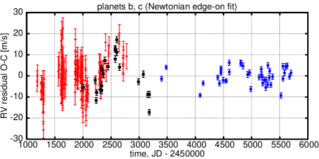
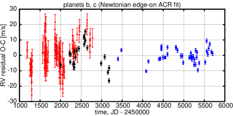
Figure 1: The RV residuals to the best fitting two-planet models of HD82943. The CORALIE data are marked as red triangles, the first Keck data-set by black squares, and the second Keck data-set by blue circles. The error bars display only the internal RV uncertainties (without the jitter).

To clarify the situation, let us consider some residual periodograms calculated with respect to different base models. They are plotted in Fig. 2. Here we plot periodograms related to each of the individual data sets as well as to the joint time series. The data-set-separated periodograms were constructed according to the method described in Baluev (2011). Namely, we assume that the probe periodic variation belongs to only a single RV data set, while the base RV model (e.g. the ones of Table 1 or Table 2) still belongs to each of them. This approach allows to easily detect various inconsistencies between different data sets, still using the full statistical power of the entire time series to fit the base model. See also (Baluev, 2013b) and references therein for a more unified description of the “residual periodograms” that we use here. Also, we note that when computing these periodograms the common orbital inclination was allowed to float to absorb as much of the residual variation as possible. The horizontal lines in the graphs of Fig. 2 show the simulated statistical levels of $1$-sigma, $2$-sigma, and $3$-sigma significance, which we discuss in more details in Section 6 below.

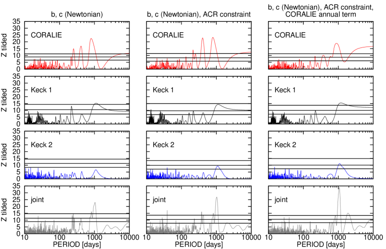
Figure 2: Residual likelihood-ratio periodograms of the HD82943 RV data for different base models, which are marked in the column titles. The periodograms correspond to the entire time series and to specific sub-data-sets (labelled in the graphs). The latter ones were constructed assuming an RV model with a probe periodicity assigned to only a particular RV data-set (labelled in each individual panel). The minimum period was increased to $10$ d from the traditional limit of $1$ d, because the time values of the CORALIE data were relatively inaccurate, as these data were scanned from a figure.

Looking at Fig. 2, we can draw the following conclusions:

1. The two-planet RV model is definitely unable to explain the full RV variation in the data. There are one or even more periodic or quasi-periodic variations in the residuals.

2. One of the main differences between the CORALIE and Keck data sets is an RV variation at the period of $\sim 400$ d. This is the only large peak that is significantly pumped up when we set up the ACR constraint (i.e. when we analyse RV residuals corresponding to a more realistic orbital model). Therefore, it is the likely source of the inconsistency.

3. Since the $\sim 400$ d period is close to the second planet’s period, it might be tempting to interpret it as some artifact of an incomplete reduction of the RV variation due to the planets c and b. This is however unlikely, because then it should exist in all three RV data sets. We interpret it as an annual variation caused by instrumental or data reduction errors related only to the CORALIE data. The periodogram peak is wide enough to be consistent with the period of $365$ d. It is already known that annual errors frequently occur in the old ELODIE RV data (Baluev, 2009, 2008b); the same may be true for CORALIE. We plot this CORALIE annual term in Fig. 3

4. Another periodogram peak persists with a period of $\sim 1100$ d. On contrary to the $400$ d peak, this one is present (and is statistically significant) in all three RV data-sets, regardless of whether we consider them jointly or separately. After removal of the CORALIE annual variation, the $\sim 1100$ d one even becomes more obvious. This convinces us that some RV variation at the period of $\sim 1100$ d does exists and it belongs to the star rather than to a specific instrument.

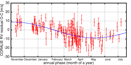
Figure 3: The best fitting CORALIE annual variation phased to its period. The RV model here is the three-planet Newtonian one with a fittable inclination. The RV contribution of the planets was subtracted from the residuals before plotting the graph, but the contribution from the annual variation was preserved.

The RV variation near the $1100$ days period was already suspected in previous studies (Beaugé et al., 2008). Its most intriguing explanation, that we analyse further in this work, is the possible existence of a third planet in the system. This hypothetical third planet would be very interesting because it appears close to the 5:2 MMR with the planet b. Thus the whole system would lie close to the three-planet 1:2:5 resonance. This is different from the 1:2:4 (Laplace) resonance suggested by Beaugé et al. (2008). The updated RV data no longer support the Laplace resonance. The Tables 3 and 4 contain the parameters of the three-planet fits that were obtained with and without the ACR constraint. Both fits correspond to an aligned apsidal corotation between the planets c and b. We interpret this as a sign of a considerably more “healthy” RV model. Although the non-ACR configuration of Table 3 still appears formally unstable, it is now very easy to slightly adjust its parameters to make it stable. In fact, now the ACR and non-ACR fits are statistically consistent with each other: we obtain only $1.5$-sigma separation from the likelihood-ratio test.

Table 3: Best fitting parameters of the HD82943 planetary system: three-planet Newtonian edge-on model with the CORALIE annual term

planetary orbital parameters and masses
	planet c	planet b	planet d
$P$ [day]	$220.080(70)$	$439.70(48)$	$1078(13)$
$K$ [m/s]	$58.5(2.3)$	$39.31(55)$	$5.30(57)$
$e$	$0.410(16)$	$0.053(63)$	$0\rm(fixed)$
$\omega$ [∘]	$117.1(1.2)$	$123.5(9.7)$	$-$
$\lambda$ [∘]	$307.3(1.1)$	$215.00(97)$	$296.0(6.0)$
$M$ [$M_{\rm Jup}$]	$1.721(78)$	$1.593(21)$	$0.290(31)$
$a$ [AU]	$0.74340(16)$	$1.17978(86)$	$2.145(17)$
$i$ [∘]	$90\rm(fixed)$
parameters of the data sets
	CORALIE	Keck 1	Keck 2
$c$ [m/s]	$8146.1(1.1)$	$-4.8(1.1)$	$-6.86(51)$
$A_{\rm sys}$ [m/s]	$8.5(1.3)$
$\tau_{\rm sys}$ [day]	$184.8(9.9)$
$\sigma_{\rm jitter}$ [m/s]	$5.63(55)$	$4.90(81)$	$2.61(34)$
r.m.s. [m/s]	$7.13$	$4.87$	$2.76$
general characteristics of the fit
$\tilde{l}$ [m/s]	$5.86$
$d$	$21$

See notes of Table 1. The additional parameters $A_{\rm sys}$ and $\tau_{\rm sys}$ represent the semiamplitude and the maximum epoch of the sinusoidal CORALIE annual variation.

Table 4: Best fitting parameters of the HD82943 planetary system: three-planet Newtonian edge-on ACR(c,b) model with the CORALIE annual term

planetary orbital parameters and masses
	planet c	planet b	planet d
$P$ [day]	$220.062(33)$	$439.586(74)$	$1072(13)$
$K$ [m/s]	$55.22(55)$	$39.86(56)$	$5.39(57)$
$e$	$0.4289(92)$	$0.1476(50)$	$0\rm(fixed)$
$\omega$ [∘]	$118.0(1.1)$	$118.0(1.1)$	$-$
$\lambda$ [∘]	$309.10(49)$	$213.56(71)$	$298.4(5.8)$
$M$ [$M_{\rm Jup}$]	$1.607(18)$	$1.600(22)$	$0.294(31)$
$a$ [AU]	$0.743340(73)$	$1.17955(13)$	$2.137(17)$
$i$ [∘]	$90\rm(fixed)$
parameters of the data sets
	CORALIE	Keck 1	Keck 2
$c$ [m/s]	$8146.1(1.1)$	$-4.8(1.0)$	$-6.89(57)$
$A_{\rm sys}$ [m/s]	$8.9(1.2)$
$\tau_{\rm sys}$ [day]	$182.4(9.3)$
$\sigma_{\rm jitter}$ [m/s]	$5.68(55)$	$4.16(71)$	$2.99(38)$
r.m.s. [m/s]	$7.21$	$4.24$	$3.10$
general characteristics of the fit
$\tilde{l}$ [m/s]	$5.91$
$d$	$21-4=17$

See notes of Table 1 and Table 2.

Here we should note that the ACR configuration of the two inner planets is perturbed by the third planet. Formally, this perturbation should slightly shift the parameters of the ACR configuration from its purely two-planet position. However, we do not take this ACR shift into account in Table 4, because it is expected to be pretty small. A rough estimation yields that the gravitational force from the planet d is smaller than $1/10$ of the one existing between the planets c and b. Therefore, the ACR constraint of Table 4 was based only on the Hamiltonian of the subsystem of the two inner planets, as if the third planet had no influence. From the other side, when we obtained the both fits of Tables 3 and 4, the gravitational perturbation from the third planet was still taken into account in full to compute the fitted RV model. In either case, dynamical simulations show that the fit of Table 4 is very close to the desired ACR state, so this fit is the one that we expected to obtain.

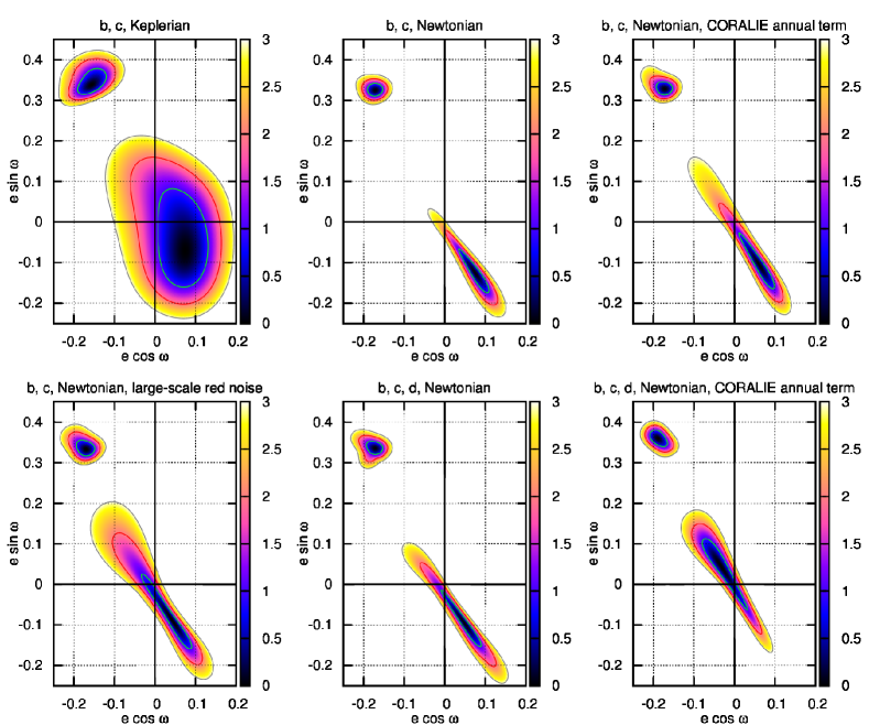
Figure 4: Confidence regions for the parameters $(e\cos\omega,e\sin\omega)$ of the HD82943 planets c and b for various RV data models. In each panel, the smaller spot in the left-top part of graph is for the planet c, and the large spot is for the planet b. The isolines correspond to the asymptotic $1$-sigma, $2$-sigma, and $3$-sigma significance levels. The type of the orbital model is marked in the titles above each plot. For the Newtonian fits we always used a coplanar orbital model with a fittable common inclination. For three-planet models the planet d was included in the $N$-body integration, but its eccentricity was always fixed at zero. See text for further details and discussion.

In view of the matters discussed above, it is interesting to track how the CORALIE annual variation and the RV contribution from the putative $\sim 1100$ days planet could distort the best fitting parameters of the main planets c and b. To do this, we consider two-dimensional confidence regions for the parameters $(e\cos\omega,e\sin\omega)$ that are plotted in Fig. 4. We give these plots for different models of the RV data. Here is what we would like to highlight:

1. The transition from the Keplerian to Newtonian RV model has a dramatic shrinking effect on the uncertainty region of $(e_{b},\omega_{b})$. However, this shrinking is severely anisotropic, and the best fitting values themselves remain rather immutable.

2. The only way to naturally obtain a stable two-planet configuration, without the use of any “brute force” like an imposed ACR constraint, is to take into account the residual long-term RV variations discussed above.

3. The stable two-planet configuration can be approached to in many ways: by adding a fittable annual variation to the CORALIE RV model, by adding the $\sim 1100$ days periodic term, or by dealing with the red-noise model using the method of Baluev (2013a). Either of these actions shifts the best fitting orbital configuration in the direction of the stable aligned ACR. However, the largest effect is obtained when the CORALIE annual term and the third planet are both included. In this case, the best fit itself migrates to the domain of aligned apses, and although this best fit is still unstable, it becomes easy to find stable configurations within its statistical uncertainties.

6 Statistical validity of the results

So far we mainly relied on analytical likelihood-ratio tests with its asymptotic chi-square distribution, and on the maximum-likelihood point estimations that are valid when the number of observations is sufficiently large. These methods are often criticised by authors who propagate the use of the Bayesian statistical methods instead. However, we believe that the weaknesses of Asymptotic Maximum-Likelihood Theory – AMLET – are often excessively exacerbated, as well as the advantages of the Bayesianism which is suggested as a replace. This has been already demonstrated in Baluev (2013a) for the case of the GJ581 planetary system, in which a rather complicated multi-planet model with correlated noise was employed. Here we aim to show that the case of HD82943 is similar in this concern, at least when all publicly available RV data are taken in the analysis.

We rely here on the Monte Carlo simulations assuming the Gaussian model of the RV noise. We do not believe that employing the bootstrap simulation, like Tan et al. (2013), would be more reliable. From Fig. 1 it is clear that the residuals to the best fitting models are anyway corrupted by some systematic variations, so it is perhaps useless to expect that shuffling of these corrupted residuals would provide a better model of the real RV noise. Besides, from Baluev (2013a) we know that the bootstrap method does not correctly handle the uncertainty of noise parameters like the jitter.

So, let us verify that we indeed can safely treat various likelihood-ratio tests obeying to the asymptotic chi-square distribution. To do this we must adopt some null hypothesis $\mathcal{H}$ (in the form of the functional model) and the alternative hypothesis $\mathcal{K}$, such that $\mathcal{H}$ is a subspace of $\mathcal{K}$ of lesser dimension. The simplest case, for example, is when we assume that $\mathcal{H}$ consists of a single point, while $\mathcal{K}$ spans the entire parametric space (for some given parametric model of the RV data). After choosing the models $\mathcal{H}$ and $\mathcal{K}$ we can run the Monte Carlo simulation (the PlanetPack algorithm described in Sect. 10.1 of Baluev 2013b) to reconstruct the distribution of the associated non-linear likelihood-ratio statistic and to compare it with the relevant chi-square distribution.

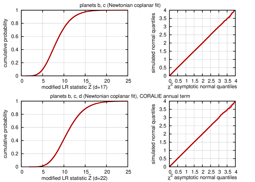
Figure 5: The distributions of the test statistic $\tilde{Z}$ from (Baluev, 2009): comparing the asymptotic $\chi^{2}$ one (thick red curves) and the simulated one (thin black curves) in each graph. Left graphs show the cumulative distribution functions (with the number of $\chi^{2}$ degrees of freedom, $d$, labelled in the abscissa). Right graphs compare the relevant normal quantiles (the $n\sigma$ significance levels). Here, the null model $\mathcal{H}$ is a single point related to some adopted “true” parameters (actually borrowed from the best fit of the real RV data), and the alternative model $\mathcal{K}$ involves a full fit of the simulated data.

In Fig. 5 we compare the simulated and analytic likelihood-ratio distributions for the case when $\mathcal{H}$ is a single point (which is treated as the true vector of the parameters), while $\mathcal{K}$ corresponds to a two-planet or a three-planet model (with a fittable common inclination in each case). We can see that the agreement is very accurate, as if these models were strictly linear.

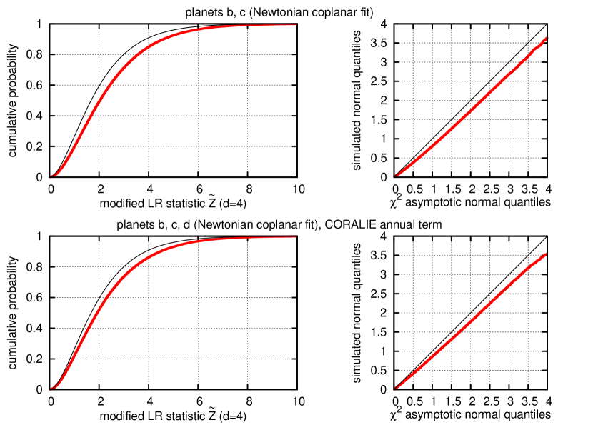
Figure 6: Same as Fig. 5, but for testing an ACR best fit against the corresponding unconstrained best fit.

Proceeding further, we verify the applicability of the asymptotic likelihood-ratio test to the task of comparing the ACR with a general non-ACR configuration. The simulation results for this test are shown in Fig. 6. In this case the alternative $\mathcal{K}$ represents the entire parametric space (for the same two models as above), while the null hypothesis $\mathcal{H}$ is a restriction of $\mathcal{K}$ to the ACR models. Now we can see some deviation between the simulated and asymptotic distribution function, but this deviation is rather marginal. In particular, the $\sim 1.5\sigma$ statistical difference between the fits of Tables 3 and 4 is now corrected to $\sim 1.3\sigma$, which is similarly insignificant. The difference of $\sim 4.2\sigma$ between the fits of Tables 1 and 2 is slightly reduced to $\sim 3.8\sigma$, which is still very large. Therefore, these correction are rather cosmetic and do not trigger any qualitative changes.

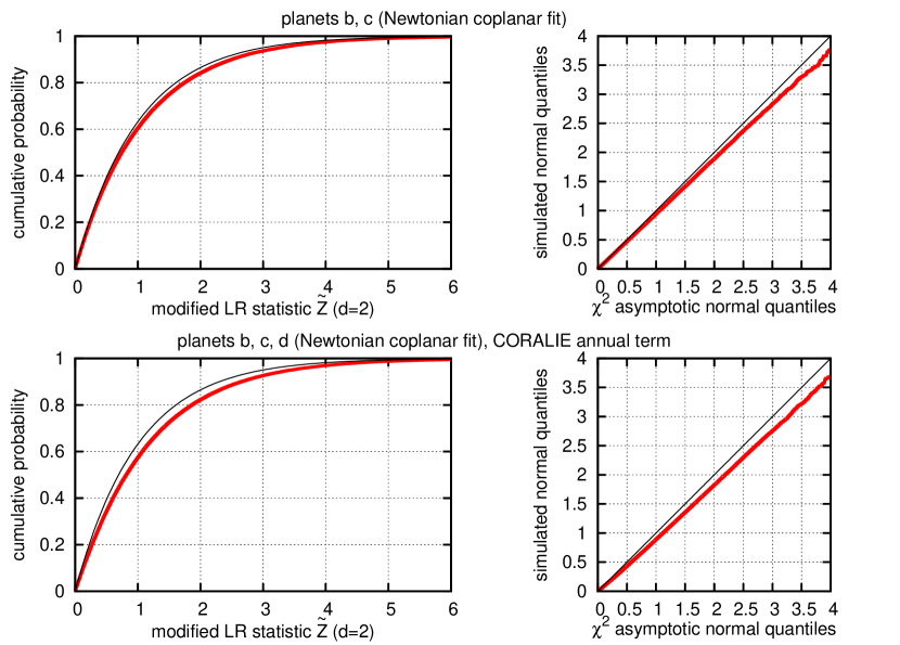
Figure 7: Same as Fig. 5, but for testing a best-fit model with fixed $(e_{b},\omega_{b})$ against the corresponding unconstrained fit. These results can be used for a more accurate calibrations of the confidence contours in Fig. 4.

Finally, we verify the calibration of the confidence contours that we plotted in Fig. 4. These confidence regions represent the level contours of the likelihood function, and they can also be treated by means of the likelihood-ratio test (Baluev, 2013b). In this case the alternative hypothesis again fills the entire parametric space, while the null hypothesis represents its restriction to some fixed values of $\omega$ and $e$ (with unrestricted other parameters). In this case the deviation between the distribution functions is even smaller than for the previous “ACR vs. non-ACR” comparison. This means that the relevant corrections to Fig. 4 would be rather unremarkable, so these confidence regions are statistically safe and reliable.

The case of the periodogram distributions did not appear that nice, however. The periodogram analog of the asymptotic chi-square likelihood-ratio distribution is the following approximation given in (Baluev, 2008a):

$${\rm FAP}(z)\lesssim M(z)\approx We^{-z}\sqrt{z},$$ (1)

where ${\rm FAP}$ is the false alarm probability to estimate, $z$ is the observed periodogram maximum, and $W$ is proportional to the settled frequency range. Formally, this formula is strictly valid only for linear models (with a single allowed non-linear frequency parameter), but for the non-linear periodograms it should be still valid in an asymptotic sense for $N\to\infty$ (Baluev, 2009).

However, the large factor $W$ in (1) scales up any non-linearity effects in the ${\rm FAP}$ to levels much larger than e.g. the small deviations seen in Figs. 5, 6, and 7 above. Monte Carlo simulations have shown that the approximation (1) works well only for the CORALIE periodogram, while for the Keck periodograms the simulated ${\rm FAP}$ is much larger than (1) predicts. This was actually expected, since the number of the Keck data is still rather small, and they are split in two even smaller independent subsets. Therefore, we decided to calibrate the periodogram significance levels of Fig. 2 with the simulated values of the ${\rm FAP}$ rather than with the analytic approximation (1). These simulations were done for the frequency range from $0$ to $0.1$ d^-1, which is the same that was used for the periodograms themselves. The simulated ${\rm FAP}$ curves are shown in Fig. 8.

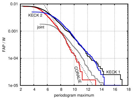
Figure 8: Simulated distributions of the periodogram maxima for periodograms in the left column of Fig. 2. The ordianate is equal to the simulated ${\rm FAP}$ divided by $W=f_{\rm max}T_{\rm eff}$, where $f_{\rm max}$ was always $0.1$ d^-1, while $T_{\rm eff}$ was different: $5534$ d for the joint data, $1245$ d for CORALIE, $1200$ d for Keck-1, and $1974$ d for Keck-2. The broken line is the graph of the function $e^{-z}\sqrt{z}$, a common asymptotic approximation based on (1). Number of Monte Carlo trials was equal to $1000$.

7 Reality of the third planet

A strong evidence in favour of the $1100$ d variation comes from its detectability in all three RV data sets that we have analysed: the CORALIE data, the Keck data before the upgrade, and the Keck data after the upgrade. Although the RV data coverage is not entirely perfect (the middle $1100$ d cycle was poorly covered), the phase of this sinusoid is more or less smoothly transferred from one data array to another (see Fig. 1 and 9). Besides, it appears difficult to naturally obtain a stable two-planet configuration from the combined time series, unless the $1100$-day variation is taken into account. This argumentation suggests that the mentioned variation does really exist and is likely caused by the star rather than by some systematic instrumental drifts or data reduction errors.

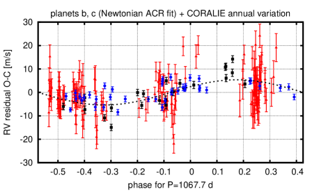
Figure 9: The two-planet RV residuals of HD82943 phased to the apparent RV period of the third planet (which is by a few days smaller than the best fitting osculating orbital period). The reference fit corresponds to the ACR two-planet Newtonian model with a fittable inclination. The data points have the same shapes as in Fig. 1.

Non-planetary interpretations of the $\sim 1100$-day RV variability are still possible. This variation could be caused by some long-term astrophysical activity phenomenon evolving on the star. In particular, the long-term stellar magnetic activity is known to generate excessive noise in the low-frequency range (Dumusque et al., 2012). In fact, it looks rather suspicious that this variation seems to fade over years: it was strong in the time of CORALIE observations, while in the latest Keck data it is more difficult to detect. However, this seems to be an apparent effect due to a more dense CORALIE data coverage and their larger number, since in the phased residuals (Fig. 9) we do not see any clear systematic differences between different data sets.

We tried to verify the long-term noise hypothesis using the red-noise analysis technique described in Baluev (2013a). Our result is that the red-noise model can easily absorb the $\sim 1100$-day variation, suppressing it well below the characteristic noise levels. The characteristic correlation timescale that the red-noise analysis algorithm reported was about a few hundred of days. Therefore, the current data are unable to distinguish the planetary and non-planetary interpretations. This ambiguity may be resolved analysing the correlation between the Doppler RV measurements and some spectral activity indicator, as Dumusque et al. (2012) have done for $\alpha$ Cen. If the same $1100$ d period is found in the star’s activity measure than we should probably retract the hypothesis of the third planet. The necessary spectral data are not publicly available, however. In any case, we still must take the relevant RV variation into account to have a more robust two-planet fit.

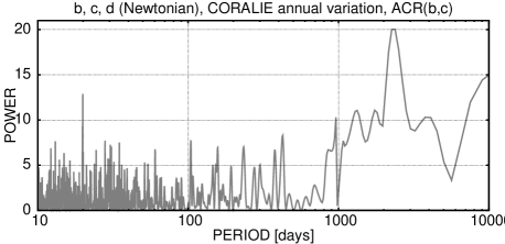
Figure 10: Residual periodogram calculated for the three-planet ACR model of HD 82943, based on the joint RV data. The system inclination to the sky plane is treated as a fittable parameter. Analogous non-ACR base model generates a similar periodogram with a slightly reduced peak at $2300$ d.

In fact, both interpretations can work together: the $1100$-day variation may be induced by the third planet indeed, and it might be also contaminated by the long-term astrophysical noise. To verify this possibility, we computed the residual periodogram with all three planets included in the base model (see Fig. 10). We can see that some residual power at long periods still remains, and it might be even statistically significant. Hwever it looks like some large-scale noise rather than a single clearly isolated period. Besides, it is remarkably smaller than the planet d peak that remained in the residuals of the analogous two-planet model (right-bottom panel of Fig. 2). We prefer to interpret the residual power in Fig. 10 as some astrophysical noise or remaining systematic instrumental errors. We definitely need more RV data to investigate this remaining residual variation more reliably.

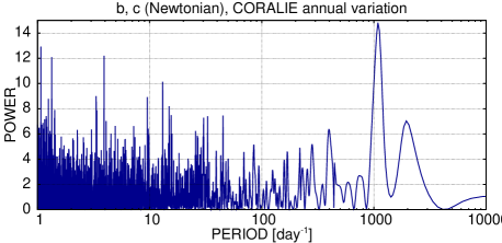
Figure 11: Residual periodogram calculated for the two-planet non-ACR model of HD 82943, based on the standalone Keck RV data (without CORALIE). The system inclination to the sky plane, $i$, is treated as a fittable parameter. The models with $i$ fixed at $90^{\circ}$ and at $20^{\circ}$ generate periodograms with a slightly higher peak at $\sim 1100$ d.

Tan et al. (2013) also noted a peak at $\sim 1100$ d in their Keck periodograms. However, their statistical analysis yielded only a marginal significance for this variation: ${\rm FAP}=0.033$ for an edge-on fit and ${\rm FAP}=0.085$ for a fit with $i=20^{\circ}$. Our work yields a remarkably more credible detection. To carry out a more direct comparison with Tan et al. (2013), in addition to the periodograms of Fig. 2 we have also computed the periodogram of the Keck data that were taken entirely alone (without CORALIE) and without imposing of any ACR constraint. The analytic formula (1) implied ${\rm FAP}\sim 10^{-3}$ for the edge-on model, ${\rm FAP}\sim 4\times 10^{-3}$ for the $i=20^{\circ}$ model, and ${\rm FAP}\sim 6\times 10^{-3}$ for the model with a floating $i$ (which still appeared close to $20^{\circ}$). Note that these ${\rm FAP}$ values are for the frequency range from $0$ to $1$ d^-1, which is $10$ times wider than that of Fig. 2. However, we have explained above that the analytic formula (1) underestimates the ${\rm FAP}$ for Keck periodograms. Therefore, we have selected the worst case of three — the model with free $i$ — and run the Monte Carlo simulation to assess the relevant ${\rm FAP}$ more reliably. We obtain the estimation of ${\rm FAP}\sim 0.016$. The relevant periodogram is shown in Fig. 11, and the graph of the associated simulated ${\rm FAP}$ is shown in Fig. 12.

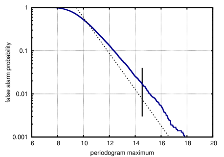
Figure 12: The solid (blue) line shows the simulated false alarm probability for the periodogram in Fig. 11. The broken line shows asymptotic approximation (1). The vertical line segment labels the abscissa position corresponding to the height of the actual periodogram peak at $P\sim 1100$ d. Number of Monte Carlo trials was equal to $10000$.

This suggests remarkably more credible detection of the planet d than what follows from Tan et al. (2013) results: e.g. the ${\rm FAP}$ is now reduced by the factor of $5$ or more. Although our Keck periodogram in Fig. 11 should be even more pessimistic than the both periodograms shown by Tan et al. (2013) in their Fig. 13, our $\sim 1100$ d peak is somewhat higher (considering all the cases relatively to their apparent noise levels). Such difference was caused, as we believe, by the following main factors. First, we used the more efficient “residual periodogram” (also known as “recursive periodogram”) instead of the “periodogram of the residuals”. The so-called residual periodogram is based on a full multi-planet fit per each computed power value, rather than on a single fit of the base model. Thus we deal with more adequate and accurate fits, which improve the periodogram detection power by pushing the real peaks up relatively to the noisy ones (Anglada-Escudé & Tuomi, 2012; Baluev, 2013b). Secondly, we used a more adequate RV noise model which involves an adaptive jitter fitting, and also allows for a more reliable relative weighting of different data sets (Baluev, 2009).

Our simulation of the Keck-only detection ${\rm FAP}$ of $1.7$ per cent (or $2.4\sigma$) for the planet d is still slightly worse than $1$ per cent (or $2.6\sigma$), which Tan et al. (2013) acknowledge as a trustable exoplanetary detection threshold. However, we re-emphasize that this long-term variation is also supported by the public CORALIE data (even after reduction of their annual variation), and the cumulative significance is much better than even the $3\sigma$ level (see Fig. 2).

8 Uncertainty of the inclination

During the preparation of this manuscript, a new observational work has appeared (Kennedy et al., 2013), where the authors consider the debris disk of HD82943 (which was originally discovered by Beichman et al. (2005)) and report a rather accurate measurement of its inclination to the sky plane: $27^{\circ}\pm 4^{\circ}$. They find this value in a good agreement with the planetary system inclination $i=20^{\circ}\pm 4^{\circ}$, as reported by Tan et al. (2013) based on the Keck RV fits. Contrary to Tan et al. (2013), the orbital inclination estimations of our work are very uncertain, with the lower typical limit on $i$ about $\sim 20^{\circ}$ and no upper limit (i.e., consistent with an edge-on orientation, $i=90^{\circ}$). The typical nominal value is $i\sim 40^{\circ}$. These results are in fact also consistent with Kennedy et al. (2013), at least we do not find any detectable disagreement. We only have to be a bit more sceptical concerning the conclusion that the disk-planets alignment is confirmed indeed; our RV data analysis just does not allow to verify this guess.

We believe that the existence of an observable outer debris disk in the system tells us indirectly that the space beyond the two robustly detectable planets is unlikely empty: the third planet or even more additional planets may be present.

Table 5: Best fitting parameters of the HD82943 planetary system: three-planet Newtonian inclined ACR(c,b) model with the CORALIE annual term

planetary orbital parameters and masses
	planet c	planet b	planet d
$P$ [day]	$220.158(33)$	$439.16(10)$	$1075(13)$
$K$ [m/s]	$55.41(54)$	$39.92(55)$	$5.42(57)$
$e$	$0.4257(93)$	$0.1460(50)$	$0\rm(fixed)$
$\omega$ [∘]	$118.0(1.1)$	$118.0(1.1)$	$-$
$\lambda$ [∘]	$309.55(50)$	$213.77(72)$	$293.5(5.7)$
$M$ [$M_{\rm Jup}$]	$3.559(40)$	$3.529(48)$	$0.653(70)$
$a$ [AU]	$0.743963(73)$	$1.18006(19)$	$2.144(17)$
$i$ [∘]	$27\rm(fixed)$
parameters of the data sets
	CORALIE	Keck 1	Keck 2
$c$ [m/s]	$8146.3(1.2)$	$-4.79(91)$	$-6.73(55)$
$A_{\rm sys}$ [m/s]	$8.7(1.2)$
$\tau_{\rm sys}$ [day]	$180.4(9.8)$
$\sigma_{\rm jitter}$ [m/s]	$5.89(56)$	$3.91(67)$	$2.93(37)$
r.m.s. [m/s]	$7.33$	$4.00$	$3.05$
general characteristics of the fit
$\tilde{l}$ [m/s]	$5.93$
$d$	$21-4=17$

The orbital inclination of the coplanar system is fixed to $27^{\circ}$, which is the debris disk inclination according to Kennedy et al. (2013). See also the notes of Table 1 and Table 2.

In Table 5 we give a refined fit with an ACR constraint and assuming the value $i=27^{\circ}$, which is now more likely than $i=90^{\circ}$, due to Kennedy et al. (2013). This configuration is stable for at least $10^{6}$ yrs. The likelihood-ratio separation between this new fit and the relevant unconstrained fit (a modification of Table 3 with free $i$) corresponds to only $1.6\sigma$ (asymptotically). The actual significance is probably even slightly smaller (see Sect. 6), so we may conclude that the RV data are entirely consistent with the coplanar three-planet ACR(b,c) configuration inclined by $27^{\circ}$ to the sky plane. In fact, such change of $i$ had only a negligible effect on the fit, except for the absolute planetary masses. Therefore, the value of $i$ does not significantly affect our main results presented so far, including e.g. the conclusions about the $1100$-day periodicity. Besides, most of these results were anyway obtained assuming a free-floating $i$, which was typically located in the range $30^{\circ}-50^{\circ}$, and this is not too far from the value provided by Kennedy et al. (2013).

However, the value of $i=27^{\circ}$ roughly doubles the planetary mass estimations, and this may have a significant effect on the planetary dynamics. In particular, the stability domains around the nominal configuration should significantly shrink. Therefore, we still need to investigate this effect.

9 Three-planet dynamics

If the $1100$-day variation is interpreted as a third planet, the entire system appears remarkably close to a 1:2:5 three-planet resonance. Although the nominal fits presented above infer that the third planet is still slightly out of the 5:2 resonance, showing a circulation of critical angles rather than a libration, the parameters of the third planet are still rather uncertain.

In particular, the eccentricity $e_{d}$ (along with the pericenter argument $\omega_{d}$) looks ill-determined: allowing it to float during the fit generates misleading overfit effects, like multiple local maxima of the likelihood function. Similarly to the HD37124 c case discussed in Baluev (2008b) or to the GJ876 e case from Baluev (2011), we find multiple local optima for the eccentric parameters $(e_{d},\omega_{d})$ at rather high $e_{d}\sim 0.3-0.4$. However, all of them are likely unreliable due to the RV model non-linearity and large uncertainties. All these local solutions may eventually disappear with more RV observations, as it expectedly occurred in the mentioned HD37124 case (Wright et al., 2011). Moreover, this effect of eccentricity bias looks frequent for exoplanets discovered by Doppler technique (Beaugé et al., 2012), and it follows from simulations of the Keplerian fits done by Cumming (2004); Zechmeister & Kürster (2009) that RV noise favours to large (and thus overestimated) eccentricity estimations. In the particular case of HD 82943 d this eccentricity bias can be also induced by the correlated astrophysical RV noise. Therefore, we conclude that the most resonable course of action is to fix $e_{d}$ at zero. The actual value of this eccentricity is in fact unconstrained.

The orbital inclination of the system, $i$, is also ill-determined and always remains statistically consistent with $90^{\circ}$, although allowing it to float during the fit does not generate any statistical degeneracies or other obvious bad effects (e.g., the simulations of Sect. 6 were all done with a floating $i$). It follows from the results by Kennedy et al. (2013) that we must pay a particular attention to the value of $i=27^{\circ}$.

The orbital period $P_{d}$ has rather good estimation accuracy, but nevertheless it may be inside as well as slightly out of the 5:2 resonance, implying a significant change in the planetary dynamics. Therefore, the uncertainties of $e_{d}$, $\omega_{d}$, $P_{d}$, and $i$ allow for a wide spread of possible dynamical regimes of the three-planet system.

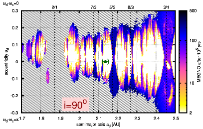
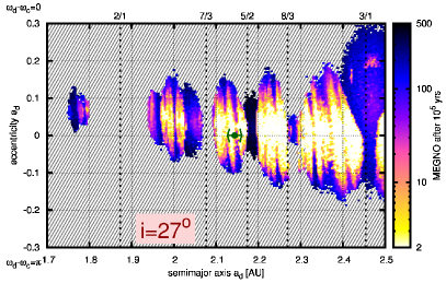
Figure 13: Dynamical maps for the neighbourhood of the planet d location (marked as a point with a error bar). The maps are obtained from the fits of Tables 4 (left) and 5 (right) by varying $e_{d}$ and $P_{d}$. The value of $\omega_{d}$ was set to either $\omega_{b}$ (upper semi-plane in each panel) or $\omega_{b}+\pi$ (lower semi-plane). The hashed region corresponds to configurations that did not survive the integration term of $10^{5}$ yrs. The MEGNO chaoticity indicator is encoded in colour. The error bar of the nominal position reflects the uncertainty of the period $P_{d}$ assuming $e_{d}=0$. Statistical uncertainties of the eccentricity $e_{d}$ exceed the ordinate range, so this eccentricity is only constrained by the stability requirement.

Our first task is to analyse the orbital stability of the region of the phase space exterior to the two known planets of the system. This will help us to constrain the location of the third planet.

A detailed analysis of the $(a_{d},e_{d})$ phase space is shown in Fig. 13. Here we show a dynamical map constructed from the numerical integration of two grids of initial conditions for the outer planet, based on the ACR configurations of Table 4 and Table 5. Positive (negative) values of $e_{d}$ correspond to aligned (anti-aligned) orbits with respect to the planet b. All initial conditions were integrated for $10^{5}$ years. The colour code shows the values of the MEGNO chaoticity indicator (Cincotta & Simó, 2000) attained during the integration interval, while the hashed domain corresponds to initial conditions that implied planetary ejections or collisions within this time-span (i.e. unstable systems).

Around $a_{d}=1.87$ AU we can clearly observe the hashed band of the 2/1 MMR. This however does not mean that the Laplace resonance 1:2:4 would inevitably lead to instability. The actual stability also depends on the angular variables that were set to particular values in Fig. 13. The plot also shows evidence of both the 5/2 and 3/1 resonances for larger semimajor axis. Other commensurabilities are also visible, although not as strong. The nominal configuration is located between the 7/3 and 5/2 MMRs. The 7/3 MMR becomes unstable for $i=27^{\circ}$ (at least for the RV-fitted values of the angles), while the 5/2 MMR remains stable.

These results indicate that it is not difficult to find a stable configuration for the third planet and in a good statistical agreement with the RV fits. However, the stability is rather sensitive to apparently small changes of the system parameters. For example, the stability domain for the non-ACR fit of Table 3 is significantly reduced in comparison with what we can see in Fig. 13. Actually, the nominal fit of Table 3 is even unstable. This indicates that apparently minor changes in the configuration of the two main planets of the system may dramatically affect the dynamics of the third planet.

The stability domains may be also reduced by assuming a smaller value for the system inclination $i$, which increases the actual planet masses. However, we found that the nominal ACR system remains stable for $i$ as small as $17^{\circ}$, so this limitation is not very important. We may note that the change of $i$ to $27^{\circ}$ remarkably transformed the structure of individual MMRs in the domain, although their general structure is still similar. In particular, the nominal solution moved very close to a high-order 22:9 (or possibly 17:7) MMR between the planets b and d, which increased the chaoticity in the entire system.

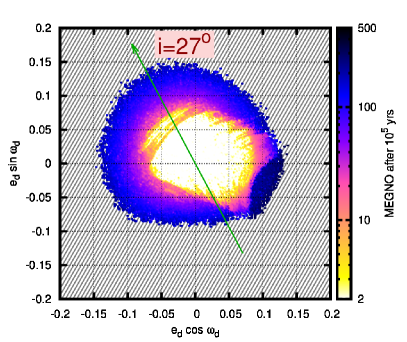
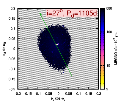
Figure 14: Dynamical maps for the ill-determined parameters $e_{d}$ and $\omega_{d}$. The left panel is based on the fit of Table 5 with non-resonant best fitting $P_{d}=1075$ d, while the right one is based on the fit with $P_{d}$ fixed at $1105$ d, the centre of the 5:2 resonance in Fig. 13. The arrows set the direction of $\omega_{b}$. The other notations are the same as in Fig. 13.

A second pair of dynamical maps is shown in Fig. 14. These are the maps for the ill-determined eccentric parameters $e_{d}$ and $\omega_{d}$ computed for the ACR fit with $i=27^{\circ}$ and a free-floating period $P_{d}$ (eventually estimated by a non-resonant value), and for the ACR fit assuming the same $i=27^{\circ}$ and fixing $P_{d}=1105$ d (at the resonance 5/2 with the planet b). We can see that the stability is generally favoured by a small $e_{d}$, although the upper limit on $e_{d}$ depends on the orientation angle $\omega_{d}$. The shape of the stability domain is different for the resonant and non-resonant value of $P_{d}$. In the non-resonant case we see clear influence of the 22:9 MMR (e.g. the chaoticity fibers in the left-top part of the stability domain). This resonance is not very strong, so the major part of the domain does not look affected by it. Nevertheless, from Fig. 13 we can see that this resonance could become a dominating factor after a small increase of $P_{d}$ with respect to the nominal value. For the 5:2 MMR case, the chaoticity is much larger, and the relevant stability domain looks featureless except for a tiny spot of regular motion near the centre. This island of regular motion appears not belonging to the three-planet MMR; below we discuss this in more details.

For the triple-resonance case, the angle $\omega_{d}$ does not describe the secular dynamics of the third planet comprehensively. In this case, the longitude $\lambda_{d}$ should also be considered, since we cannot directly average the resonant Hamiltonian over it. Although the value of $\lambda_{d}$ is determined relatively well (at least, with a much better accuracy than $\omega_{d}$), we must plot a dynamical map by varying this longitude to understand the position of the nominal system in the phase space.

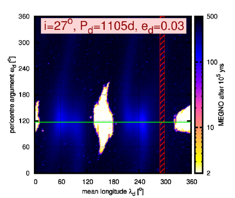
Figure 15: Dynamical map for the angular parameters $\lambda_{d}$ and $\omega_{d}$ for the three-planet MMR. The maps are based on the same fit as the one used for the right frame of Fig. 14, now setting $e_{d}=0.03$. The horizontal (green) line shows the position of $\omega_{b}$. The hashed vertical band shows the one-sigma uncertainty range of the best fitting $\lambda_{d}$ (assuming that $\omega_{d}$ is indetermined). The other notations are the same as in Fig. 13.

If Fig. 15 we show the map plotted for the parameters $\lambda_{d}$ and $\omega_{d}$. The map was based on an ACR(b,c) fit fixing $i=27^{\circ}$, $P_{d}=1105$ d, $e_{d}=0$, and with $e_{d}$ manually moved (without further refitting) from $0$ to $0.03$. In this plane most of the initial conditions lead to very chaotic motion, although still stable within the time-span covered by our integration. Our attention is mainly attracted by two remarkable spots of regular motion near $\lambda_{d}=150^{\circ}$ and $350^{\circ}$. The detailed investigation showed that this regular motion is not truly resonant: one or both critical angles, related to planet d, circulate. Only the 2:1 resonance is preserved here, while the 5:2 one is broken. Therefore, these spots represent some breaches in the structure of the three-planet MMR. We cannot tell anything clear about the topology of these breaches in the phase space. It is an open question, whether they represent some disconnected inner caves or they look like pipes passing through the MMR domain. In the remaining (truly resonant) part of the map there are a few small domains with a smaller degree of chaoticity (those having a bit lighter colour). The typical Lyapunov time over the map is only $\sim 250$ yr, but it rises to $\sim 1000$ yr in these domains. These domains are probably related to some triple-ACR configurations like the one appearing in Sect. 10 below. However, the value of $\lambda_{d}$ suggested by the RV data is located between these domains, where the chaoticity is high. As the uncertainty of $\lambda_{d}$ is rather small, it appears that our RV fits are inconsistent with these moderately-chaotic domains.

The simultaneous presence of fully resonant (1:2:5) as well as only partly resonant (1:2) configurations in Fig. 15 indicates that this map represents a slice of the phase space taken close to the relevant separatrix. This explains why most of these initial conditions are very chaotic — the chaos is typically located near a separatrix. We believe that the chaoticity may be reduced by seeking a suitable adjustment of the orbital elements of the two inner planets. The ACR constraint used to obtain the above fits neglected the perturbalitions from the third planet. Taking them into account would slightly shift the estimated ACR equilibria. This would not significantly affect the quality of the RV fit, but the long-term dynamics might change dramatically.

So far, we were unable to find in the vicinity of the nominal fit any regular or at least low-chaotic motion simultaneously belonging to the three-planet MMR. All our configurations with regular dynamics are not entirely resonant. We however did not try to vary the parameters of the two inner planets, which may have a significant effect on the dynamics of the outermost one. Besides, some real planetary systems do show a chaotic dynamics (see e.g. the GJ 876 case discussion by Martí et al. 2013), so we should not assume that the dynamics of the HD 82943 planetary system have to be regular. We only need it to be long-term stable.

10 Three-planet migration

The primary goal of this section is to demonstrate that the 1:2:5 three-planet resonance can be naturally established via the mechanism of the planetary migration.

But first of all, let us investigate in more detail the dynamical status of the two main resonant planets c and b. We compare the general layout of the dynamical ACR families of the 2:1 resonance (Beaugé et al., 2003) with the actual best-fitting configurations and with the associated parametric uncertainty regions in the plane $(e_{c},e_{b})$. These results are plotted in Fig. 16, where we use a three-planet coplanar model with a free-floating orbital inclination. Each point in the $(e_{c},e_{b})$ plain corresponds to some ACR configuration. We have three domains, corresponding to different types of stable ACRs: the symmetric anti-aligned family (labelled as “s$><$”), the symmetric aligned one (“symmetric$<<$”), and the asymmetric ACRs.

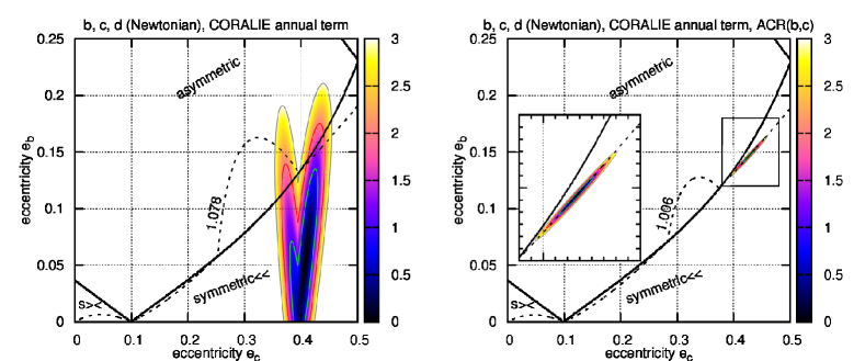
Figure 16: The eccentricities of the major planets in the HD82943 system: comparing the non-ACR (left) and the ACR solution (right). The asymptotic $1$-, $2$-, $3$-sigma confidence regions inferred by the corresponding orbital model, and the surrounding layout of the ACR configurations are displayed together. The thick solid lines separate different types of ACRs for the 2/1 MMR case. The thick dashed line in each graph shows an iso-family of the ACRs with a constant planet mass ratio, taken from the corresponding RV fit.

Each ACR configuration implies, in particular, a fixed value of the planetary mass ratio that must be held. Thus, for a given mass ratio we can plot a corresponding iso-family of ACRs. Such isolines are very important, because they may serve as evolutionary tracks of the system during the planet migration phase (Beaugé et al., 2006). In each of the two panels of Fig. 16 we plot a single such isoline that corresponds to the relevant best fitting mass ratio. We can see that both these isolines pass through all three types of ACRs. Therefore, this system could undergo an asymmetric ACR state in some past and then switched back to the symmetric regime.

Planetary migration was simulated using a standard $N$-body code based on a Bulirsch-Stoer integration routine, plus a Stokes-type exterior force (Beaugé et al., 2006) with specified values for the $e$-folding times for the semimajor axis ($\tau_{a}$) and eccentricity ($\tau_{e}$). We assumed that only the exterior (hypothetical) planet suffered the migration. Both inner planets suffered no orbital decay, except the indirect one, induced by the outer planet once the 3-planet resonance was established. However, we did include an eccentricity damping on the c and b planets, just to keep their eccentricities fixed.

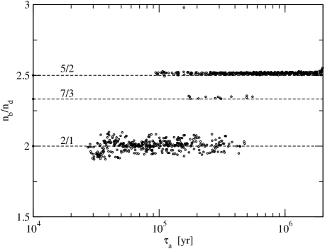
Figure 17: Final mean-motion ratios between the two outer planets $m_{b}$ and $m_{d}$, as a function of the orbital decay $e$-folding time, for a total of $1798$ $N$-body runs with planetary migration acting on the outer mass. The main MMRs attained by the planets are shown in horizontal dashed lines.

We analysed several initial conditions and migration rates. There is evidence (e.g. Beaugé et al., 2008; Martí et al., 2013) that 3-planet resonances may be fairly fragile with small stability domains, so it is possible that the probability of finding stable configurations is not high. On the other hand, it is well known that the commensurability in which the bodies are ultimately captured depend on the migration rate and initial semimajor axis ratio (Nelson & Papaloizou, 2002; Rein et al., 2010).

The initial orbits of $m_{c}$ and $m_{b}$ were chosen equal to those shown in Table 4, while the semimajor axis and eccentricity of the outer planet were chosen randomly in the intervals $a_{d}\in[2.36,2.38]$ AU and $e_{d}\in[0,0.02]$. Although the limits of both intervals were small, they guaranteed a random distribution of the angular variables at each resonance, allowing us to estimate the capture probabilities in each commensurability. The values of $a_{d}$ are interior to the 3/1 resonance, but outside the 5/2. Finally, the migration rates were also chosen randomly in the interval $\tau_{a}\in[10^{3},2\times 10^{6}]$, while $\tau_{e}$ was chosen such that $\tau_{e}/\tau_{a}=100$, a value expected for Type-1 migration in laminar isothermal disks (Ogihara & Ida, 2009).

Fig. 17 shows the final $P_{d}/P_{b}$ ratio for $1798$ initial conditions and migration rates. The integration time was a function of $\tau_{a}$, and the runs were stopped once a stable configuration was reached with constant mean-motion ratios. In all cases we checked that the two inner planets remained locked in the 2/1 MMR.

As expected, the final MMR attained by the outer planet depends on $\tau_{a}$. We can roughly identify four different intervals. For very slow migration rates ($\tau_{a}>5\times 10^{5}$ yrs), practically all the fictitious systems ended trapped in 3-planet resonances, and in all cases the two outer planets were locked in the 5/2 MMR. For slightly faster migrations (down to $\tau_{a}\sim 10^{5}$ yrs), some initial conditions crossed the 5/2 resonance, most being trapped in the 2/1. However, a few were also captured in the 7/3, while $\sim 10$ per cent of the initial conditions lead to unstable orbits and were ejected from the system.

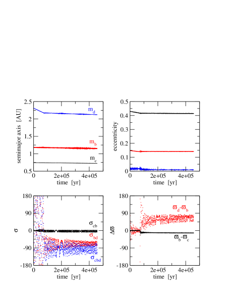
Figure 18: A simulation of the planet d migration and trapping of all three bodies in the 5:2:1 multiple resonance. The resonant angles are defined in (2).

For even lower decay times ($\tau_{a}<10^{5}$ yrs), the 5/2 resonance seemed unable to counteract the dissipative force and all stable configurations correspond to the 2/1 MMR, defining thus a Laplace resonance between all three planets. However, about half of the runs lead to unstable orbits. Finally, no resonance capture was observed for $\tau_{a}<3\times 10^{4}$ yrs.

Summarising, the 5:2:1 three-planet resonance seems a natural outcome of this type of simple $N$-body experiments, as long as the orbital decay rate is sufficiently slow. Whether this could indeed be the case is a matter of dispute. From the analytical estimates by Tanaka et al. (2002), for a minimum mass solar nebula and typical disk properties, $\tau_{a}$ is estimated to be of the order of $\sim 10^{4}$ yrs for planets with masses comparable to the estimated value of $m_{d}$. However, it is important to keep in mind that planetary migration is not well understood and it is believed that migration rates, especially for Type-I, should have been lower than what linear theories for laminar disks predict. For example, MHD turbulence could delay the orbital decay as much as two orders of magnitude (Nelson & Papaloizou, 2004; Alibert et al., 2005), leading to values more compatible with planetary formation. So, the values $\tau_{a}\sim 10^{5}$ yrs or even higher are plausible.

Figure 18 shows an example of the trapping of third planet in a 5/2 MMR with the second one, and the consequent locking of all three planets in the 5:2:1 multiple resonance. The two top frames show the time variation of the semimajor axes (left) and eccentricities (right). The triple commensurability is attained in less than $10^{5}$ yrs, after which all planets continue to migrate together.

The bottom left-hand graph shows the evolution of the resonant angles, defined as:

$$\sigma_{cb} = 2\lambda_{b}-\lambda_{c}-\varpi_{c},$$

$$\sigma_{bd} = 5\lambda_{d}-2\lambda_{b}-3\varpi_{b},$$

$$\sigma_{cbd} = 5\lambda_{d}-8\lambda_{b}+3\lambda_{c}.$$ (2)

where $\sigma_{cbd}$ is the critical angle of the 3-planet resonance. The angle $\sigma_{cb}$ is the leading critical angle of the 2/1 MMR between the planets c and b, and it is always librating. Before the triple-resonance is established, $\sigma_{cb}$ librates around zero, as expected from a symmetric ACR solution. However, after the third planet becomes resonant, the libration centre switches to an asymmetric value, although still close to zero. The angle $\sigma_{bd}$ is the one associated to the 5/2 resonance between b and d. It circulates before the resonance trapping, and librates around an asymmetric value after that. The same is noted in $\sigma_{cbd}$. Note that from e.g. the fit of Table 4 we have $\sigma_{cbd}=-9^{\circ}\pm 29^{\circ}$ and $\sigma_{cbd}=-34^{\circ}\pm 29^{\circ}$ for Table 5, so the real orbital configuration is not necessarily a three-planet ACR like the one appearing in Fig. 18.

Finally, the bottom right-hand plot shows the behaviour of the difference in pericenters. Again, $\varpi_{b}-\varpi_{c}$ starts librating around zero, but changes to an asymmetric libration after the system is trapped in the 5:2:1 MMR. The same is also noted for $\varpi_{d}-\varpi_{b}$.

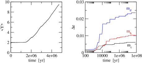
Figure 19: Left: MEGNO value $\langle Y\rangle$ as function of time for an initial condition in the 5:2:1 MMR. Right: Evolution of $\Delta e$ for the three planets during a $10^{8}$ yrs $N$-body integration.

To check whether the stability of this orbit is due to the gas, we took the state of the system at $t=2\times 10^{5}$ yrs, considered those as new initial conditions and integrated it again without gas effects for $10^{8}$ yrs. We also calculated the MEGNO chaos indicator for the run. Results are shown in the left plot of Fig. 19. The value of $\langle Y\rangle$ starts close to $2$ (indicating a regular motion) but after $\sim 10^{6}$ yrs it begins to linearly grow. This indicates chaotic motion, although only noticeable after $10^{6}$ yrs, indicating that the chaos is weak. A linear fit of the value of $\langle Y\rangle$ after this time indicates a maximum Lyapunov exponent also of the order of $10^{6}$ yrs.

To analyse the stability of this chaotic configuration, we tried to estimate any diffusion in the action space. This was done calculating the evolution of $\Delta e$, defined as the amplitude of the eccentricity of each planet. For regular motion, $\Delta e$ should be constant. For chaotic but stable motion, this quantity should also be constant or bounded. Results are shown in the right-hand plot of Fig. 19. We observe a secular increase in all values of $\Delta e$, larger for the outer planet and smaller for the inner body. The values, however, remain small. If there is any orbital instability, it should only be observable for timescales much larger than the age of the star.

11 Conclusions

We believe that the existence of the $1100$-days variation in the RV data for HD82943 is if not convincing, at least plausible. Moreover, it is likely that this variation was caused by some agent related to the star itself rather than to a particular instrument. However, we reiterate that we still do not insist on the planetary interpretation of this variation. It can also be a hint of some long-term noise caused by the star’s activity.

The planetary interpretation leads us to an extremely interesting dynamical system in the three-planet resonance 1:2:5. This would be, to our concern, the second such candidate system. The previous one was the system of KOI 806/Kepler-30, detected by transits and transit timing variations (Tingley et al., 2011), although later data suggested that its third planet is significantly out of the $5:2$ MMR (Fabrycky et al., 2012).

What concerns the major planets b and c, their dynamics is likely close to the aligned ACR located near the border with asymmetric ACRs. But the RV fitting uncertainties still do not constrain the dynamical regime of HD 82943 d well. The third planet may be inside as well as slightly out of the 5:2 MMR with the planet b, implying different dynamics. Initial conditions with non-resonant third planet often lead to a regular and stable motion. However, inside the three-planet 1:2:5 resonance, we could not find any regular or low-chaotic motion that would be more or less consistent with the RV data. It is nonetheless known that chaotic configurations are not necessarily inacceptable, since chaos does not necessarily imply instability. For example, the GJ 876 planetary system demonstrates a chaotic but stable motion in the Laplace resonance (Martí et al., 2013).

We find that the three-planet 1:2:5 resonance may represent a rather natural outcome of the planetary orbital migration. If this three-planet resonance will be further confirmed, this may place significant constraints on the parameters of the migration process, like the characteristic migration rate.

Whether the third planet exists or not, there is one interesting matter concerning the two inner planets. Their nominal configuration corresponds to a symmetric aligned ACR located very close to the boundary with the domain of asymmetric ACRs. Moreover, from Fig. 16 we may suspect that this system could have passed through the asymmetric corotation regime somewhen in the past, during the planetary migration stage.

According to Beaugé et al. (2006), once the migration is driven by a dissipative adiabatic force, it should follow the isolines of the constant mass ratio shown in Fig. 16. Therefore, during the migration there could be two rather abrupt switches between the symmetric and asymmetric corotation modes. Due to large eccentricities and masses of the planets c and b, these bifurcations would basically represent a dynamical catastrophe for other planets in the system, should they exist there in that epoch. As a result, some of these planets could be ejected out of the system or could fall on the star. Such a conclusion provides a nice theoretical explanation of the spectroscopic observations that detected an unusually high Lithium-6 abundance in the atmosphere of HD82943 (Israelian et al., 2001). This chemical anomaly was hypothetically interpreted as an evidence that some planets could fall on the host star in the past, enriching it with Lithium-6. We can see that the ACR-sticky migration mechanism by Beaugé et al. (2006) provides a good explanation of how such a catastrophe could be actually triggered.

References

- Alibert et al. (2005) Alibert Y., Mordasini C., Benz W., Winisdoerffer C., 2005, A&A, 434, 343
- Anglada-Escudé & Tuomi (2012) Anglada-Escudé G., Tuomi M., 2012, AA, 548, A58
- Baluev (2008a) Baluev R. V., 2008a, MNRAS, 385, 1279
- Baluev (2008b) Baluev R. V., 2008b, Celest. Mech. Dyn. Astron., 102, 297
- Baluev (2009) Baluev R. V., 2009, MNRAS, 393, 969
- Baluev (2011) Baluev R. V., 2011, Celest. Mech. Dyn. Astron., 111, 235
- Baluev (2012) Baluev R. V., 2012, MNRAS, 422, 2372
- Baluev (2013a) Baluev R. V., 2013a, MNRAS, 429, 2052
- Baluev (2013b) Baluev R. V., 2013b, Astronomy & Computing, 2, 18
- Beaugé et al. (2003) Beaugé C., Ferraz-Mello S., Michtchenko T. A., 2003, ApJ, 593, 1124
- Beaugé et al. (2012) Beaugé C., Ferraz-Mello S., Michtchenko T. A., 2012, Research in Astron. Astrophys., 12, 1044
- Beaugé et al. (2008) Beaugé C., Giuppone C., Ferraz-Mello S., Michtchenko T. A., 2008, MNRAS, 385, 2151
- Beaugé et al. (2006) Beaugé C., Michtchenko T. A., Ferraz-Mello S., 2006, MNRAS, 365, 1160
- Beichman et al. (2005) Beichman C. A., Bryden G., Rieke G. H., Stansberry J. A., Trilling D. E., Stapelfeldt K. R., Werner M. W., Engelbracht C. W., Blaylock M., Gordon K. D., Chen C. H., Su K. Y. L., Hines D. C., 2005, ApJ, 622, 1160
- Cincotta & Simó (2000) Cincotta P. M., Simó C., 2000, A&AS, 147, 205
- Cumming (2004) Cumming A., 2004, MNRAS, 354, 1165
- Dumusque et al. (2012) Dumusque X., Pepe F., Lovis C., Ségransan D., Sahlmann J., Benz W., Bouchy F., Mayor M., Queloz D., Santos N., Udry S., 2012, Nature, 491, 207
- Fabrycky et al. (2012) Fabrycky D. C., Ford E. B., Steffen J. H., Rowe J. F., Carter J. A., Moorhead A. V., Batalha N. M., Borucki W. J., Bryson S., Buchhave L. A., Christiansen J. L., Ciardi D. R., Cochran W. D., Endl M., Fanelli M. N., Fischer D., Fressin F., Geary J., Haas M. R., Hall J. R., Holman M. J., Jenkins J. M., Koch D. G., Latham D. W. et al., 2012, ApJ, 750, 114
- Ferraz-Mello et al. (2005a) Ferraz-Mello S., Michtchenko T. A., Beaugé C., 2005a, ApJ, 621, 473
- Ferraz-Mello et al. (2005b) Ferraz-Mello S., Michtchenko T. A., Beaugé C., Callegari N., 2005b, Lect. Not. Phys., 683, 219
- Goździewski et al. (2008) Goździewski K., Breiter S., Borczyk W., 2008, MNRAS, 383, 989
- Goździewski & Konacki (2006) Goździewski K., Konacki M., 2006, ApJ, 647, 573
- Goździewski et al. (2005) Goździewski K., Konacki M., Maciejewski A. J., 2005, ApJ, 622, 1136
- Goździewski & Maciejewski (2001) Goździewski K., Maciejewski A. J., 2001, ApJ, 563, L81
- Israelian et al. (2001) Israelian G., Santos N. C., Mayor M., Rebolo R., 2001, Nature, 411, 163
- Ji et al. (2003) Ji J., Kinoshita H., Liu L., Li G., Nakai H., 2003, Celest. Mech. Dyn. Astron., 87, 113
- Kennedy et al. (2013) Kennedy G. M., Wyatt M. C., Bryden G., Wittenmyer R., Sibthorpe B., 2013, MNRAS, 436, 898
- Lee et al. (2006) Lee M. H., Butler R. P., Fischer D. A., Marcy G. W., Vogt S. S., 2006, ApJ, 641, 1178
- Martí et al. (2013) Martí J. G., Giuppone C. A., Beaugé C., 2013, MNRAS, 433, 928
- Mayor et al. (2004) Mayor M., Udry S., Naef D., Pepe F., Queloz D., Santos N. C., Burnet M., 2004, A&A, 415, 391
- Michtchenko et al. (2006) Michtchenko T. A., Beaugé C., Ferraz-Mello S., 2006, Celest. Mech. Dyn. Astron., 94, 411
- Nelson & Papaloizou (2002) Nelson R. P., Papaloizou J. C. B., 2002, MNRAS, 333, L26
- Nelson & Papaloizou (2004) Nelson R. P., Papaloizou J. C. B., 2004, MNRAS, 350, 849
- Ogihara & Ida (2009) Ogihara M., Ida S., 2009, ApJ, 699, 824
- Rein et al. (2010) Rein H., Papaloizou J. C. B., Kley W., 2010, A&A, 510, A4
- Tan et al. (2013) Tan X., Payne M. J., Lee M. H., Ford E. B., Howard A. W., Johnson J. A., Marcy G. W., Wright J. T., 2013, ApJ, 777, id101
- Tanaka et al. (2002) Tanaka H., Takeuchi T., Ward W. R., 2002, ApJ, 565, 1257
- Tingley et al. (2011) Tingley B., Palle E., Parviainen H., Deeg H. J., Zapatero Osorio M. R., Cabrera-Lavers A., Belmonte J. A., Rodriguez P. M., Murgas F., Ribas I., 2011, A&A, 536, id. L9
- Vuong (1989) Vuong Q. H., 1989, Econometrica, 57, 307
- Wright et al. (2011) Wright J. T., Veras D., Ford E. B., Johnson J. A., Marcy G. W., Howard A. W., Isaacson H., Fischer D. A., Spronck J., Anderson J., Valenti J., 2011, ApJ, 730, id93
- Zechmeister & Kürster (2009) Zechmeister M., Kürster M., 2009, A&A, 496, 577