Semi-Decentralized Approximation of Optimal Control of Distributed Systems Based on a Functional Calculus

Abstract

This paper discusses a new approximation method for operators which are solution to an operational Riccati equation (ORE). The latter is derived from the theory of optimal control of linear problems posed in Hilbert spaces. The approximation is based on the functional calculus of self-adjoint operators and the Cauchy formula. Under a number of assumptions the approximation is suitable for implementation on a semi-decentralized computing architecture in view of real-time control. Our method is particularly applicable to problems in optimal control of systems governed by partial differential equations with distributed observation and control. Some relatively academic applications are presented for illustration. More realistic examples relating to microsystem arrays have already been published.

1 Introduction

This work is a contribution to the area of semi-decentralized optimal control of large linear distributed systems for real-time applications. It applies to systems modeled by linear partial differential equations with observation and control distributed over the whole domain. This is a strong assumption, but it does not mean that actuators and sensors are actually continuously distributed. The models satisfying such assumption may be derived by homogenization of systems with periodic distribution of actuators and sensors.

In this paper we consider two classes of systems, those with bounded control and bounded observation operators as in R. Curtain and H. Zwart [6], and those with unbounded control but bounded observation operators as in H.T. Banks and K. Ito [2]. In an example, we show how the method may also be applied to a particular boundary control problem. We view possible applications in the field of systems including a network of actuators and sensors, see for instance [13] dedicated to arrays of Atomic Force Microscopes.

We consider four linear operators $A,$ $B,$ $C$, $S$, and the Linear Quadratic Regulator (LQR) problem stated classically as a minimization problem,

$$\mathcal{J}\left(z_{0},{\mathbf{u}}\right) = \min\limits_{u\in U}\mathcal{J}\left(z_{0},u\right),$$ (1)

$$\text{with}~{}\mathcal{J}\left(z_{0},u\right) = \int_{0}^{+\infty}\left\|Cz\right\|_{Y}^{2}+\left(Su,u\right)_{U}~{}dt,$$ (2)

constrained by a state equation,

$$\frac{dz}{dt}\left(t\right)=Az\left(t\right)+Bu\left(t\right)\quad\text{for }t>0\quad\text{and }z\left(0\right)=z_{0}\text{.}$$ (3)

Under usual assumptions there exists a unique solution ${\mathbf{u}}=-S^{-1}B^{\ast}Pz$, where $P$ is a solution of the operational Riccati equation (ORE),

$$A^{\ast}P+PA-PBS^{-1}B^{\ast}P+C^{\ast}C=0\text{.}$$ (4)

In the framework of [6], $A:D(A)\subset Z\mapsto Z,$ $B:U\mapsto Z,$ $C:Z\mapsto Y$, $S:U\mapsto U$ and consequently $P:Z\mapsto Z$ for some linear spaces $Z,$ $U$ and $Y$. To derive our semi-decentralized realization of $Pz$, we further assume that there exists a linear self-adjoint operator $\Lambda:X\mapsto X$, three one-to-one mappings

$$\Phi_{Z}:X^{n_{Z}}\mapsto Z,\quad\Phi_{U}:X^{n_{U}}\mapsto U\quad\text{and }\Phi_{Y}:X^{n_{Y}}\mapsto Y,$$ (5)

with appropriate integers $n_{Z},$ $n_{U}$ and $n_{Y},$ and four continuous matrix-valued functions $\lambda\mapsto a(\lambda),$ $\lambda\mapsto b(\lambda)$, $\lambda\mapsto c(\lambda)$ and $\lambda\mapsto s(\lambda)$ such that

$$A=\Phi_{Z}a(\Lambda)\Phi_{Z}^{-1},\quad B=\Phi_{Z}b(\Lambda)\Phi_{U}^{-1},\quad C=\Phi_{Y}c(\Lambda)\Phi_{Z}^{-1}\quad\text{and }S=\Phi_{U}s(\Lambda)\Phi_{U}^{-1}.$$ (6)

We notice that the functions of the self-adjoint operator $\Lambda$ used in the above formulae are defined using spectral theory of self-adjoint operators (having a real spectrum) with compact or not compact resolvent so that to encompass bounded and unbounded domains. From (6), it follows that the Riccati operator $P$ is factorized as

$$P=\Phi_{Z}p(\Lambda)\Phi_{Z}^{-1},$$ (7)

where $\lambda\mapsto p(\lambda)$ is a continuous function, solution of the algebraic Riccati equation (ARE)

$$a^{T}\left(\lambda\right)p+pa\left(\lambda\right)-pb\left(\lambda\right)s^{-1}\left(\lambda\right)b^{T}\left(\lambda\right)p+c^{T}\left(\lambda\right)c\left(\lambda\right)=0\text{.}$$ (8)

Our goal is reached once separate efficient semi-decentralized approximations of $\Phi_{Z}$, $p(\Lambda)$ and $\Phi_{Z}^{-1}$ are provided for the realization of $P$ through (7). This is generally not an issue for $\Phi_{Z}$ and for $\Phi_{Z}^{-1},$ then the point is the semi-decentralized approximation of $p(\Lambda)$. It might be build by a polynomial approximation,

$$p_{N}(\Lambda)=\sum_{k=0}^{N}d_{k}\Lambda^{k},$$ (9)

or a rational approximation,

$$p_{N}(\Lambda)=\frac{\sum\limits_{k=0}^{N^{N}}d_{k}\Lambda^{k}}{\sum\limits_{k^{\prime}=0}^{N^{D}}d_{k^{\prime}}^{\prime}\Lambda^{k^{\prime}}}\text{.}$$ (10)

Then, for practical implementations, the operator $\Lambda$ could be replaced by a discretizations $\Lambda_{h},$ with parameter $h.$ We emphasize that the formulae (9) or (10) yield large approximation errors, with respect to $h,$ due to the high powers of $\Lambda_{h}$. To overcome this defect, we use an approximation based on the Cauchy integral which requires to know the poles of $p$. In practice, we first approximate the function $\lambda\mapsto p(\lambda)$ by a polynomial approximation or a rational approximation $p_{N}(\lambda)$ with degrees $N$ or $(N^{N},N^{D})$ sufficiently high to insure a very small error. When $p_{N}$ is known its poles also, so we can state the Cauchy formula for $p_{N}(\Lambda)$. This yields to introduce the equations of the complex function $v=v_{1}+iv_{2}$ for each input $z\in Z,$

$$(\xi-\Lambda)v=-i\xi^{\prime}p_{N}\left(\xi\right)z,$$ (11)

where $\xi:(0,2\pi)\rightarrow\mathbb{C}$ is the contour of the Cauchy formula. Denoting by $v^{\ell}$ the solution corresponding to a quadrature point $\xi_{\ell}$ of the contour and $\omega_{\ell}$ some quadrature weights, the final approximation of $p(\Lambda)z$ is

$$p_{N,M}(\Lambda)z=\frac{1}{2\pi}\sum_{\ell=1}^{M}\omega_{\ell}v_{1}^{\ell}.$$ (12)

Remark that the number $M$ of quadrature points is the only important parameter governing the approximation error. For real-time computation, the expression of $p_{N}$ is pre-computed, so the approximation cost is also governed by $M$ only. With this method, we do not observe a lack of precision when $\Lambda$ is replaced by its discretizations $\Lambda_{h}$ and $M$ is large. In the sequel, we show that the same derivation can be done directly for $Qz=-S^{-1}B^{\ast}Pz$ provided that the isomorphisms $\Phi_{Z}$ and $\Phi_{U}$ are also some functions of $\Lambda.$

This approach based on functional calculus is relatively simple, but in each case it requires to determine the isomorphisms (5). The theory has already been applied in [25] to a LQG control problem with a bounded operator $B$ that is not a function of $\Lambda$. It has been shown how the control approximation can be implemented through a distributed electronic circuit. In [19] and [13] it has also been applied to a one-dimensional array of cantilevers with regularly spaced actuators and sensors for which the operator $C$ is not a function of $\Lambda$. The underlying model was derived with a multiscale method, an implementation of the semi-decentralized control was provided in the form of a periodic network of resistors, and the numerical validations of the complete strategy was carried out. In the present paper, we illustrate the theory with four simpler examples ranging from a simple heat equation with internal bounded control and observation operators, a heat equation with an unbounded control operator, a vibrating Euler-Bernoulli beam, and a heat equation with a boundary controls.

We notice that our method together improves and generalizes a previous paper [15]. It was related to a specific application, namely vibration control problem for a plate with a periodic distribution of piezoelectric actuators and sensors. There, the general isomorphisms (5) and the general factorization (6) were not introduced, and $p(\Lambda)$ was approximated by a polynomial as in (9) which were severely limiting the accuracy of the approximation. In both papers, the control method is a LQR, but the theory is applicable to Riccati equations that may arise in a number of other control problem, for instance for $H_{2}$ or $H_{\infty}$ dynamic compensators. Other extensions are also possible, for instance, we may want to deal with functions of a non self-adjoint operator $\Lambda$. In such a case, another functional calculus, like these in [21] or in [12], could be used instead of the spectral theory. Other frameworks for control problems of infinite dimensional systems could also be used, for instance this of [17] for optimal control with unbounded observations and unbounded controls.

Other techniques have already been established, see [1], [22], [14], [7], [16] and the references therein. But they are mostly focused on the infinite length systems, see [1], [22], [14] and [16] for systems governed by partial differential equations, and [7] for discrete systems. Finally, in [18] we developed another theoretical framework based on the diffusive realization applicable to a broad range of linear operators on bounded or unbounded domains. In principle this approach allows to cover general distributed control problems with internal or boundary control. However, in this first paper in the subject, only one-dimensional domains and linear operational equations (e.g. Lyapunov equations) are covered.

The paper is organized as follows. Notations and basic definitions are recalled in Section 2. In Section 3 the abstract approximation method is stated in the framework of bounded control and observation operators. The framework of unbounded control operators is treated in Section 4. Some extensions are outlined in Section 5. Most proofs are concentrated in Section 6. The illustrative examples are detailed in Section 7 and finally the paper is concluded by Section 8.

2 Preliminary Results and Notations

The norm and the inner product of an Hilbert space $E$ are denoted by $||.||_{E}$ and $(.,.)_{E}.$ For a second Hilbert space $F,$ $\mathcal{L}(E,F)$ denotes the space of continuous linear operators from $E$ to $F.$ In addition, $\mathcal{L}(E,E)$ is denoted by $\mathcal{L}(E).$ One says that $\Phi\in\mathcal{L}(E,F)$ is an isomorphism from $E$ to $F$ if $\Phi$ is one-to-one and if its inverse is continuous.

Since the approximation method of $P$ is based on the concept of matrices of functions of a self-adjoint operator, this section is devoted to their definition. Let $\Lambda$ be a self-adjoint operator on a separable Hilbert space $X$ with domain $D(\Lambda)$, we denote by $\sigma(\Lambda)$ its spectrum and by $I_{\sigma}=(\sigma_{\min},\sigma_{\max})\subset\mathbb{R}$ an open interval that includes $\sigma(\Lambda)$. We recall that if $\Lambda$ is compact then $\sigma(\Lambda)$ is bounded and is only constituted of eigenvalues $\lambda_{k}.$ They are the solutions to the eigenvalue problem $\Lambda\phi_{k}=\lambda_{k}\phi_{k}$ where $\phi_{k}$ is an eigenvector associated to $\lambda_{k}$ chosen normed in $X$, i.e. such that $||\phi_{k}||_{X}=1$. For a given real valued function $f$, continuous on $I_{\sigma}$, $f(\Lambda)$ is the linear self-adjoint operator on $X$ defined by

$$f(\Lambda)z=\sum_{k=1}^{\infty}f(\lambda_{k})z_{k}\phi_{k}\quad\text{where }z_{k}=(z,\phi_{k})_{X},$$

with domain $D(f(\Lambda))=\{z\in X~{}|~{}\sum\limits_{k=1}^{\infty}\left|f(\lambda_{k})z_{k}\right|^{2}~{}<\infty\}.$ Then, if $f$ is a $n_{1}\times n_{2}$ matrix of real valued functions $f_{ij},$ continuous on $I_{\sigma}$, $f(\Lambda)$ is a matrix of linear operators $f_{ij}(\Lambda)$ with domain

$$D(f(\Lambda))=\{z\in X^{n_{2}}~{}|~{}\sum\limits_{k=1}^{\infty}\sum\limits_{j=1}^{n_{2}}|f_{ij}(\lambda_{k})(z_{j})_{k}|^{2}~{}<\infty\quad\forall i=1\ldots n_{1}\}.$$

In the general case, where $\Lambda$ is not compact and where $f$ is still a continuous function, the self-adjoint operator $f(\Lambda)$ is defined on $X$ by the Stieltjes integral

$$f(\Lambda)=\int_{-\infty}^{+\infty}\lambda~{}dE_{\lambda},$$

and its domain is $D(f(\Lambda))=\{z\in X~{}|~{}\int_{-\infty}^{+\infty}|f(\lambda)|^{2}\text{ }d||E_{\lambda}z||_{X}^{2}~{}<\infty\}$ where $E_{\lambda}$ is the spectral family associated to $\Lambda$, see [8]. When $f$ is a matrix, $f(\Lambda)$ is a matrix of linear operators with entries defined by the above formula and with domain

$$D(f(\Lambda))=\{z\in X^{n_{2}}~{}|~{}\int_{-\infty}^{+\infty}\sum\limits_{j=1}^{n_{2}}|f_{ij}(\lambda)|^{2}~{}d||E_{\lambda}z_{j}||_{X}^{2}~{}<\infty\quad\forall i=1\ldots n_{1}\}.$$

3 Bounded Control Operators

In this section, we state the approximation result in the framework of bounded input operators. We follow the mathematical setting [6] of the LQR problem (1-3). So, $A$ is the infinitesimal generator of a continuous semigroup on a separable Hilbert space $Z$ with dense domain $D(A)$, $B\in\mathcal{L}(U,Z)$, $C\in\mathcal{L}(Z,Y)$ and $S\in\mathcal{L}(U,U)$ where $U$ and $Y$ are two Hilbert spaces. We assume that $(A,B)$ is stabilizable and that $(A,C)$ is detectable, in the sense that there exist $Q\in\mathcal{L}(Z,U)$ and $F\in\mathcal{L}(Y,Z)$ such that $A-BQ$ and $A-FC$ are the infinitesimal generators of two uniformly exponentially stable continuous semigroups. For each $z_{0}\in Z$ the LQR problem (1-3) admits a unique solution ${\mathbf{u}}=-S^{-1}B^{\ast}Pz$ where $P\in\mathcal{L}(Z)$ is the unique self-adjoint nonnegative solution of the ORE

$$\left(A^{\ast}P+PA-PBS^{-1}B^{\ast}P+C^{\ast}C\right)z=0$$ (13)

for all $z\in D(A).$ The adjoint $A^{\ast}$ of the unbounded operator $A$ is defined from $D(A^{\ast})\subset Z$ to $Z$ by the equality $(A^{\ast}z,z^{\prime})_{Z}=(z,Az^{\prime})_{Z}$ for all $z\in D(A^{\ast})$ and $z^{\prime}\in D(A)$. The adjoint $B^{\ast}\in\mathcal{L}(Z,U)$ of the bounded operator $B$ is defined by $(B^{\ast}z,u)_{U}=(z,Bu)_{Z}$, the adjoint $C^{\ast}\in\mathcal{L}(Y,Z)$ being defined similarly.

Now, we state specific assumptions for the approximation method. Here, $\Lambda$ is a given self-adjoint operator on a separable Hilbert space $X$ which is chosen to be easily approximable on a semi-decentralized architecture. Generally, $\Lambda$ is chosen with regard to $A,$ then $\Phi_{Z}$ and $\Phi_{U}$ can be chosen so that to have also a natural semi-decentralized approximation.

Assumption (H1).

There exist three integers $n_{Z},$ $n_{U}$ and $n_{Y}\in\mathbb{N}^{\ast}$, three isomorphisms $\Phi_{Z}\in\mathcal{L}(X^{n_{Z}},Z),$ $\Phi_{U}\in\mathcal{L}(X^{n_{U}},U)$ and $\Phi_{Y}\in\mathcal{L}(X^{n_{Y}},Y)$ and four matrices of functions $a(\lambda)\in\mathbb{R}^{n_{Z}\times n_{Z}},$ $b(\lambda)\in\mathbb{R}^{n_{Z}\times n_{U}}$, $c(\lambda)\in\mathbb{R}^{n_{Y}\times n_{Z}}$ and $s(\lambda)\in\mathbb{R}^{n_{U}\times n_{U}}$ continuous on $I_{\sigma}$ such that

$$A=\Phi_{Z}a(\Lambda)\Phi_{Z}^{-1},\quad B=\Phi_{Z}b(\Lambda)\Phi_{U}^{-1},\quad C=\Phi_{Y}c(\Lambda)\Phi_{Z}^{-1}\quad\text{and}\quad S=\Phi_{U}s(\Lambda)\Phi_{U}^{-1}.$$

One of the consequences of this assumption, for a system governed by a partial differential equation posed in a domain $\Omega,$ is that both the control and the observation must be distributed throughout the domain, in conformity with what has been stated from the beginning.

Remark 3.1.

1. In case where all operators are function of $\Lambda$, then the isomorphisms $\Phi$ are or not useful or can be chosen as function of $\Lambda$. In both cases $P$ is also a function $p$ of $\Lambda$.

2. Introducing the isomorphisms $\Phi_{Z}$, $\Phi_{Y}$ and $\Phi_{U}$ allows to deal with problems where operators $A$, $B$ and $C$ are not functions of $\Lambda$.

3. When control is distributed over the entire domain Assumption (H1) is generally satisfied. In Section 7.3, there is an example of observation operator $C$ that is not a function of $\Lambda$, while in the paper [19] it is the case for $B$ the control operator.

4. For boundary control or observation problems, it is impossible to find such isomorphisms. Nevertheless, in Subsection 7.4 we show how to proceed to address some boundary control problems.

5. Multi-scale models with controls at the micro scale, as in [19] and [13], are also possible applications.

We introduce the ARE

$$a^{T}\left(\lambda\right)p+pa\left(\lambda\right)-pb\left(\lambda\right)s^{-1}\left(\lambda\right)b^{T}\left(\lambda\right)p+c^{T}\left(\lambda\right)c\left(\lambda\right)=0\text{.}$$ (14)

Assumption (H2).

For all $\lambda\in I_{\sigma}$, the ARE (14) admits a unique nonnegative symmetric solution denoted by $p(\lambda)$.

Remark 3.2.

This assumption is stronger than the typical sufficient condition for the mere existence of a solution to the Riccati equation [give ref].

We make the following choices for the inner products of $Z$, $U$ and $Y$:

$$\left(z,z^{\prime}\right)_{Z}=\left(\Phi_{Z}^{-1}z,\Phi_{Z}^{-1}z^{\prime}\right)_{X^{n_{Z}}},~{}\left(u,u^{\prime}\right)_{U}=\left(\Phi_{U}^{-1}u,\Phi_{U}^{-1}u^{\prime}\right)_{X^{n_{U}}}~{}\text{and}~{}\left(y,y^{\prime}\right)_{Y}=\left(\Phi_{Y}^{-1}y,\Phi_{Y}^{-1}y^{\prime}\right)_{X^{n_{Y}}}.$$

Thus $P$, $Q$ and $p$, $q$ are related as follows.

Theorem 3.3.

If (H1) and (H2) are fulfilled then

$$P=\Phi_{Z}~{}p(\Lambda)~{}\Phi_{Z}^{-1}\quad\text{and}\quad{\mathbf{u}}=-Qz$$

where the controller $Q$ admits the factorization $Q=\Phi_{U}q(\Lambda)\Phi_{Z}^{-1}$ with $q(\Lambda)=s^{-1}(\Lambda)b^{T}(\Lambda)p(\Lambda)\text{.}$

Now, we focus on a semi-decentralized approximation of $Q$ which reduces to provide such an approximation for $q(\Lambda)$. We restrict the presentation to the case of bounded operators $\Lambda$ since they have a bounded spectra. This is sufficient for applications to systems governed by partial differential equations in bounded domains.

Assumption (H3).

The operator $\Lambda$ is bounded and its spectrum $\sigma(\Lambda)$ is bounded, so there exists $R>0$ with $\sigma(\Lambda)\subset(-R,R).$

This assumption can be relaxed, see Section 5.

Assumption (H4).

The operators $\Phi_{Z}$, $\Phi_{Z}^{-1},$ $\Lambda$ and $(\xi I-\Lambda)^{-1}$ admit semi-decentralized approximations for all $\xi\in\mathbb{C}$ with $|\xi|=R$.

Now, we introduce two successive approximations $q_{N}(\Lambda)$ and $q_{N,M}(\Lambda)$ of $q(\Lambda)$ that play a key role in our method.

$\vartriangleright$ The rational approximation $q_{N}(\Lambda)$: Since the interval $I_{\sigma}$ is bounded, each entries $q_{ij}$ of the matrix $q$ admits a rational approximation on $I_{\sigma}$. This defines a matrix of rational approximations of $q(\lambda)$,

$$q_{N}\left(\lambda\right)=\frac{\sum\limits_{k=0}^{N^{N}}d_{k}\lambda^{k}}{\sum\limits_{k^{\prime}=0}^{N^{D}}d_{k^{\prime}}^{\prime}\lambda^{k^{\prime}}},$$ (15)

to be understood componentwise, so each $d_{k}$, $d_{k^{\prime}}^{\prime}$ is a matrix and $N=\left(N^{N},N^{D}\right)$ is a pair of matrices of polynomial degrees. The particular case $N^{D}=0$ corresponds to a classical polynomial approximation. For any $\eta>0$ the degrees of approximations can be chosen so that the uniform estimate

$$\sup_{\lambda\in I_{\sigma}}\left|q\left(\lambda\right)-q_{N}\left(\lambda\right)\right|\leq C_{1}\left(q\right)\eta$$ (16)

holds.

$\vartriangleright$ Approximation $q_{N,M}(\Lambda)$ by quadrature of the Cauchy integral: For any complex valued function $g(\theta)$ continuous on $[0,2\pi],$ we introduce $I_{M}(g)=\displaystyle\sum\limits_{\ell=1}^{M}\omega_{\ell}g(\theta_{\ell})$ a quadrature rule for the integral $I\left(g\right)=\int_{0}^{2\pi}g\left(\theta\right)~{}d\theta$, $(\theta_{\ell})_{\ell}$ denoting the nodes of a regular subdivision of $[0,2\pi]$ and $\omega_{\ell}$ the associated quadrature weights. The quadrature rule is assumed to satisfy an error estimate as

$$\left|I\left(g\right)-I_{M}\left(g\right)\right|\leq C_{2}\left(g\right)\eta\text{.}$$ (17)

For $z\in X^{n_{Z}}$ and $\xi=\xi_{1}+i\xi_{2}$ a sufficiently regular complex contour enlacing $\sigma(\Lambda)$ and not surrounding any pole of $q_{N}.$ We parameterize it by a parameter varying in $[0,2\pi]$. We further introduce the solution $(v_{i})_{i=1,2}$ of the system

$$\left\{\begin{array}[]{c}\xi_{1}v_{1}-\xi_{2}v_{2}-\Lambda v_{1}=\Re e\left(-i\xi^{\prime}q_{N}\left(\xi\right)\right)z,\\ \xi_{2}v_{1}+\xi_{1}v_{2}-\Lambda v_{2}=\Im m\left(-i\xi^{\prime}q_{N}\left(\xi\right)\right)z,\end{array}\right.$$ (18)

and the second approximation of $q(\Lambda)$ through its realizations

$$q_{N,M}(\Lambda)z=\frac{1}{2\pi}\sum_{\ell=1}^{M}\omega_{\ell}v_{1}^{\ell}\text{.}$$ (19)

We notice that two approximations $p_{N}$ and $p_{N,M}$ of the function $p$ can be constructed by following the same steps. The next theorem states the approximations of the operators $P$ and $Q.$

Theorem 3.4.

Under the assumptions (H1-H4), $P$ and $Q$ can be approximated by one of the two semi-decentralized approximations

$$P_{N}=\Phi_{Z}p_{N}\left(\Lambda\right)\Phi_{Z}^{-1} \quad Q_{N}=\Phi_{U}q_{N}\left(\Lambda\right)\Phi_{Z}^{-1}$$ and

$$\text{or }P_{N,M}=\Phi_{Z}p_{N,M}\left(\Lambda\right)\Phi_{Z}^{-1} \quad Q_{N,M}=\Phi_{U}q_{N,M}\left(\Lambda\right)\Phi_{Z}^{-1}\text{.}$$ and

Moreover, for any $\eta>0,$ there exist $N$ and $M$ such that

$$\left\|P-P_{N}\right\|_{\mathcal{L}\left(Z\right)} \leq C_{3}\eta\text{, }\left\|Q-Q_{N}\right\|_{\mathcal{L}\left(Z,U\right)}\leq C_{3}^{\prime}\eta$$

$$\text{and }\left\|P-P_{N,M}\right\|_{\mathcal{L}\left(Z\right)} \leq C_{4}\eta\text{, }\left\|Q-Q_{N,M}\right\|_{\mathcal{L}\left(Z,U\right)}\leq C_{4}^{\prime}\eta,$$

$C_{3}$, $C_{3}^{\prime}$ and $C_{4},$ $C_{4}^{\prime}$ being independent of $\eta,$ $N$ and $M$.

Remark 3.5.

In the case of a polynomial approximation, i.e. $N^{D}=0$, we can set a circle as contour $\xi(\theta)=Re^{i\theta}$. For actual rational approximations, the contour must leave the poles outside, so we choose an ellipse centered at $\frac{R_{1}}{2}$ parameterized by $\xi(\theta)=\frac{R_{1}}{2}\left(1+\cos\left(\theta\right)\right)+iR_{2}\sin\left(\theta\right)$ where $R_{1}$ and $R_{2}$ are for the major and minor radii and $R_{2}$ is small enough.

Remark 3.6.

The approximation of $p$ used in [15] is based on Taylor series, so it is applicable only if the interval $I_{\sigma}$ is sufficiently small. The approximation proposed in our paper does not suffer from this drawback.

Remark 3.7.

In case where the solution $P$ of a Riccati equation is a kernel operator (see [20] for optimal control of systems governed by partial differential equations) i.e. $Pz(x)=\int_{\Omega}\overline{p}(x,x^{\prime})z(x^{\prime})dx^{\prime}$ and if $\Lambda$ is a compact operator then the kernel may be decomposed on a basis of eigenvectors of $\Lambda$,

$$\overline{p}(x,x^{\prime})=\sum\limits_{k=1}^{\infty}p(\lambda_{k})\phi_{k}(x)\phi_{k}(x^{\prime}).$$

The truncation technique used in [1] can be applied to build a semi-decentralized approximation of $P$. However, when the decay of $\overline{p}$ is not very fast, this technique is not efficient, see for example the case $p(\lambda)=\lambda$ that may yield from a LQR problem.

For concrete real-time computations one can use either of the two formulae (15) or (19) given that both are semi-decentralized, but we prefer the second since it does not make use of powers of $\lambda.$ The reason will become clearer when discretizing. In a real-time computation, the realization $q_{N,M}(\Lambda)z$ requires solving $M$ systems (18) corresponding to $M$ complex values $\xi(\theta_{\ell})$. So the parameter $M$ is essential to evaluate the cost of our algorithm. The matrix $q_{N}$ is pre-computed off-line once and for all and we choose $N$ sufficiently large that $q_{N}$ is a very good approximation of $q$. Consequently, $M$ is the only parameter that influences the accuracy of the method, except the parameter space discretization that is discussed now.

The end of the section is devoted to spatial discretization. For the sake of simplicity, the interval is meshed with regularly spaced nodes separated by a distance $h$.

$\vartriangleright$ Spatial discretization with polynomial approximation: First, we introduce $\Lambda_{h}^{k}$ the finite differences discretizations of $\Lambda^{k}$, with $k=1\cdots N$. For $N^{D}=0$, the discretization $q_{N,h}$ of $q_{N}$ in (15) can be written as

$$q_{N,h}z_{h}=\sum_{k=0}^{N}d_{k}\Lambda_{h}^{k}z_{h},$$

where $z_{h}$ is the vector of nodal values of $z$. Their discretization yields very high errors because the powers of $\Lambda$. This can be avoided by using the Cauchy formula, i.e. the equation (18).

$\vartriangleright$ Spatial discretization with Cauchy formula approximation: For each quadrature point $\xi:=\xi_{1,\ell}+i\xi_{2,\ell}$, the discrete approximation $\left(v_{1,h}^{\ell},v_{2,h}^{\ell}\right)$ of $\left(v_{1}^{\ell},v_{2}^{\ell}\right)$ is the solution of the discrete set of equations

$$\left\{\begin{array}[]{c}\xi_{1,\ell}v_{1,h}^{\ell}-\xi_{2}v_{2,h}^{\ell}-\Lambda_{h}v_{1,h}=\Re e\left(-i\xi_{\ell}q_{N}\left(\xi_{\ell,\ell}\right)\right)z_{h},\\ \xi_{2,\ell}v_{1,h}^{\ell}+\xi_{1,\ell}v_{2,h}^{\ell}-\Lambda_{h}v_{2,h}=\Im m\left(-i\xi_{\ell}q_{N}\left(\xi_{\ell}\right)\right)z_{h}\text{.}\end{array}\right.$$ (20)

Thus we deduce the discretization $q_{N,M,h}$ of the approximation $q_{N,M}$ in (19),

$$q_{N,M,h}z_{h}=\frac{1}{2\pi}\sum_{\ell=1}^{M}\omega_{\ell}v_{1,h}^{\ell}\text{.}$$ (21)

Under the Assumption (H4), we introduce $\Phi_{U,h}$ and $\Phi_{Z,h}$ the semi-decentralized approximations of $\Phi_{U}$ and $\Phi_{Z}$. So, the approximations of ${\mathbf{u}}_{N}$ and ${\mathbf{u}}_{N,M}$ by a spatial discretization are

$${\mathbf{u}}_{N,h}=-\Phi_{U,h}q_{N,h}\Phi_{Z,h}^{-1}z_{h}\quad\text{and}\quad{\mathbf{u}}_{N,M,h}=-\Phi_{U,h}q_{N,M,h}\Phi_{Z,h}^{-1}z_{h}.$$ (22)

This constitutes two different final semi-decentralized approximations of ${\mathbf{u}}$.

Remark 3.8.

The approximations ${\mathbf{u}}_{N,h}$ and ${\mathbf{u}}_{N,M,h}$ are given in the general case where the isomorphisms $\Phi_{Z}$ and $\Phi_{U}$ are not function of $\Lambda$ only. Therefore, we use our approximation technique to represent $q(\Lambda)$. In some cases $\Phi_{Z}$ and $\Phi_{U}$ are function of $\Lambda$ and then $Q$ is also and the approximation is developed directly on it that we denote by $k(\Lambda)$,

$${\mathbf{u}}_{N,h}=-k_{N,h}(\Lambda)z_{h}\quad\text{and}\quad{\mathbf{u}}_{N,M,h}=-k_{N,M,h}(\Lambda)z_{h}\text{.}$$ (23)

In the case where $\Phi_{Z}$ and $\Phi_{U}^{-1}Q$ are functions of $\Lambda$ then the approximation is developed on $\Phi_{U}^{-1}Q$, we will also denote it by $k(\Lambda)$ without risk of confusion,

$${\mathbf{u}}_{N,h}=-\Phi_{U,h}k_{N,h}(\Lambda)z_{h}\quad\text{and}\quad{\mathbf{u}}_{N,M,h}=-\Phi_{U,h}k_{N,M,h}(\Lambda)z_{h}.$$

4 Unbounded Control Operators

When the input operator $B$ is unbounded from $U$ to $Z$ and the observation operator $C$ is bounded from $Z$ to $Y$, we use the framework of [2] where $V$ is another Hilbert space, $V^{\prime}$ is its dual space with respect to the pivot space $Z,$ $A\in\mathcal{L}(V,V^{\prime}),$ $B\in\mathcal{L}(U,V^{\prime})$ and $C\in\mathcal{L}(Z,Y)$. A number of other technical assumptions are not detailed here. The state equations are written in the sense of $V^{\prime}$ with $z_{0}\in Z.$ The optimal control is ${\mathbf{u}}=-B^{\ast}Pz$ where $P$ is the unique nonnegative solution of the Riccati operatorial equation

$$\left(A^{\ast}P+PA-PBB^{\ast}P+C^{\ast}C\right)v=0,$$ (24)

for all $v\in V.$ The adjoint $A^{\ast}\in\mathcal{L}(V,V^{\prime})$ is defined by $\left\langle A^{\ast}v,v^{\prime}\right\rangle_{V^{\prime},V}=\left\langle v,Av^{\prime}\right\rangle_{V,V^{\prime}}$ when $B^{\ast}\in\mathcal{L}(V^{\prime},U)$ is defined as the adjoint of a bounded operator. We keep the same inner products for $Z,$ $U$ and $Y$, and those of $V$ and $V^{\prime}$ are

$$\left(v,v^{\prime}\right)_{V}=\left(\Phi_{V}^{-1}v,\Phi_{V}^{-1}v^{\prime}\right)_{X^{n_{Z}}}\quad\text{and}\quad\left(v,v^{\prime}\right)_{V^{\prime}}=\left(\Phi_{V^{\prime}}^{-1}v,\Phi_{V^{\prime}}^{-1}v^{\prime}\right)_{X^{n_{Z}}}.$$

Moreover, we choose $J=\Phi_{V}\Phi_{V^{\prime}}^{-1}$ as the canonical isomorphism from $V^{\prime}$ to $V$ and the duality product between $V$ and $V^{\prime}$ is

$$\left\langle v,v^{\prime}\right\rangle_{V,V^{\prime}}=(v,Jv^{\prime})_{V}.$$

Assumption (H1’).

Same statement as (H1) excepted that

$$A=\Phi_{V^{\prime}}a(\Lambda)\Phi_{V}^{-1}\quad\text{and}\quad B=\Phi_{V^{\prime}}b(\Lambda)\Phi_{U}^{-1}$$

where $\Phi_{V}\in\mathcal{L}(X^{n_{Z}},V)$ and $\Phi_{V^{\prime}}\in\mathcal{L}(X^{n_{Z}},V^{\prime})$ are two additional isomorphisms. Moreover,

$$\Phi_{V}=\phi_{V}(\Lambda)\text{, }\quad\Phi_{Z}=\phi_{Z}(\Lambda)\quad\text{and}\quad\Phi_{V^{\prime}}=\phi_{V^{\prime}}(\Lambda)$$

are some functions of $\Lambda$.

Here, the ARE is

$$\phi_{V^{\prime}}\left(\lambda\right)a^{T}\left(\lambda\right)~{}p~{}\phi_{V^{\prime}}^{-1}\left(\lambda\right)\phi_{V}\left(\lambda\right)+\phi_{V}\left(\lambda\right)~{}p~{}a\left(\lambda\right)$$

$$-\phi_{V}\left(\lambda\right)~{}p~{}b\left(\lambda\right)s^{-1}\left(\lambda\right)b^{T}\left(\lambda\right)~{}p~{}\phi_{V^{\prime}}^{-1}\left(\lambda\right)\phi_{V}\left(\lambda\right)$$ (25)

$$+\phi_{Z}\left(\lambda\right)c^{T}\left(\lambda\right)c\left(\lambda\right)\phi_{Z}^{-1}\left(\lambda\right)\phi_{V}\left(\lambda\right)=0\text{.}$$

Assumption (H2’).

For all $\lambda\in I_{\sigma}$, the ARE (25) admits a unique nonnegative solution denoted by $p(\lambda)$.

Theorem 4.1.

If (H1’,H2’) are fulfilled, then

$$P=\Phi_{V}~{}p(\Lambda)~{}\Phi_{V^{\prime}}^{-1}\quad\text{and}\quad{\mathbf{u}}=-Qz$$

where $Q$ admits the factorization $Q=\Phi_{U}q(\Lambda)$ with $q(\Lambda)=b^{T}(\Lambda)\phi_{V^{\prime}}^{-1}\phi_{V}p(\Lambda)\phi_{V^{\prime}}^{-1}.$

The following assumptions are necessary for the semi-decentralized approximation of $P$.

Assumption (H4’).

Same statement that (H4) completed by $\Phi_{V}$, $\Phi_{V^{\prime}}$ and $\Phi_{V^{\prime}}^{-1}$ admit a semi-decentralized approximation.

In the next statement, the approximations $q_{N}$ and $q_{N,M}$ of $q$ are built according to the formulae (15) and (19).

Theorem 4.2.

Under the Assumptions (H1’,H2’,H3,H4’), $P$ and $Q$ can be approximated by one of the two semi-decentralized approximations

$$P_{N}=\Phi_{V}p_{N}(\Lambda)\Phi_{V^{\prime}}^{-1} Q_{N}=\Phi_{U}q_{N}(\Lambda),$$ and

$$\text{or }P_{N,M}=\Phi_{V}p_{N,M}(\Lambda)\Phi_{V^{\prime}}^{-1} Q_{N,M}=\Phi_{U}q_{N,M}(\Lambda).$$ and

Moreover, for any $\eta>0,$ there exist $N$ and $M$ such that

$$\left\|P-P_{N}\right\|_{\mathcal{L}(V^{\prime},V)} \leq C_{3}\eta,\quad\left\|Q-Q_{N}\right\|_{\mathcal{L}(V^{\prime},U)}\leq C^{\prime}_{3}\eta,$$

$$\text{and }\left\|P-P_{N,M}\right\|_{\mathcal{L}(V^{\prime},V)} \leq C_{4}\eta,\quad\left\|Q-Q_{N,M}\right\|_{\mathcal{L}(V^{\prime},U)}\leq C^{\prime}_{4}\eta,$$

$C_{3}$, $C^{\prime}_{3}$, $C_{4}$ and $C^{\prime}_{4}$ being independent of $\eta,$ $N$ and $M$.

Remark 4.3.

An example of unbounded control operators is given in the Subsection 7.2.

The approximations of ${\mathbf{u}}$ and ${\mathbf{u}}_{h}$ are constructed using the same method as in the case of bounded control operators.

5 Extensions

In this section, we mention possible extensions of the theoretical framework presented above.

The same strategy applies directly to dynamic estimators and compensators derived by the $H_{2}$ to the $H_{\infty}$ theories. For instance, the condition $\rho\left(P\overline{P}\right)<\gamma$ on the spectral radius of the product of the solution of the two Riccati equation can be expressed under the form of a condition on the spectral radius of the product of two parameterized matrices $\rho\left(p\left(\lambda\right)\overline{p}\left(\lambda\right)\right)<\gamma$ for all $\lambda\in I_{\sigma}$, see Lemma 6.2 (6).

The spectral theory of self-adjoint operators has been chosen for its relative simplicity. We are aware of its limitation, so we mention possible extensions based on more general functional calculi like these developped in [21] or [12] to cite only two.

Other frameworks for the well-posedness of the LQR problem can be used. In particular, this of [17] for optimal control with unbounded observation and control may be incorporated in this approach.

6 Proofs

First, we remark that for $E$ and $F$ two Hilbert spaces and $\Phi$ an isomorphism from $E$ to $F,$ if $F$ is equipped with the inner product $(z,z^{\prime})_{F}=(\Phi^{-1}z,\Phi^{-1}z^{\prime})_{E}$ then $\Phi^{\ast}=\Phi^{-1}$. In the next lemma, we state few functional calculus properties.

Lemma 6.1.

For $\Lambda$ a self-adjoint operator on a separable Hilbert space $X$, and for $f$, $g$ two functions continuous on $I_{\sigma}$

1. $f(\Lambda)$ is self-adjoint;

2. for $\mu\in\mathbb{R}$, $(\mu f)(\Lambda)=\mu f(\Lambda)$ on $D(f(\Lambda))$;

3. $(f+g)(\Lambda)=f(\Lambda)+g(\Lambda)$ on $D(f(\Lambda))\cap D(g(\Lambda))$;

4. $g(\Lambda)f(\Lambda)=(g$ $f)(\Lambda)$ when the range of $f(\Lambda)$ is included in $D(g(\Lambda))$;

5. if $f\neq 0$ in $I_{\sigma}$ then $f(\Lambda)^{-1}$ exists and is equal to $\frac{1}{f}(\Lambda)$;

6. if $f(\lambda)\geq 0$ for all $\lambda\in I_{\sigma}$ then $f(\Lambda)\geq 0$;

7. $||f(\Lambda)x||_{X}^{2}$ $\leq$ $\sup\limits_{\lambda\in I_{\sigma}}|f(\lambda)|^{2}||x||_{X}^{2}$ for all $x\in D(f(\Lambda))$.

Proof.

The proofs of the first five statements can be found in [8]. We prove (6) i.e. that $\displaystyle\sum\limits_{i,j=1}^{n}(f_{ij}(\Lambda)z_{j},z_{i})_{X}\geq 0$. First, assume that $I_{\sigma}$ is bounded. We recall that for a function $g$ continuous on $I_{\sigma}$ and for $z\in X,$ the integral $\int_{\sigma_{\min}}^{\sigma_{\max}}g(\lambda)dE_{\lambda}z$ is defined as the strong limit in $X$ of the Riemann sums, see [8], $\displaystyle\sum\limits_{k=1}^{p}g(\lambda_{k}^{\prime})(E_{\lambda_{k+1}}-E_{\lambda_{k}})z$ when $\max\limits_{k}|\lambda_{k+1}-\lambda_{k}|$ vanishes, where $\lambda_{k}^{\prime}\in[\lambda_{k},\lambda_{k+1}]$ and $\sigma_{\min}=\lambda_{1}<\lambda_{2}...<\lambda_{p}=\sigma_{\max}$. When $I_{\sigma}$ is not bounded, we use a subdivision of a bounded interval $I_{\widetilde{\sigma}}=(\widetilde{\sigma}_{\min},\widetilde{\sigma}_{\max})$ and the integral $\int_{\sigma_{\min}}^{\sigma_{\max}}g(\lambda)dE_{\lambda}z$ is defined by passing to the limit in the integral bounds. Let us establish that the Riemann sum $\displaystyle\sum\limits_{i,j=1}^{n}\sum\limits_{k=1}^{p}f_{ij}(\lambda_{k}^{\prime})((E_{\lambda_{k+1}}z_{j},z_{i})-(E_{\lambda_{k}}z_{j},z_{i}))$ is nonnegative, so the result will follow by passing to the limit. Since $(E_{\lambda_{k+1}}z_{j},z_{i})-(E_{\lambda_{k}}z_{j},z_{i})=((E_{\lambda_{k+1}}-E_{\lambda_{k}})z_{j},z_{i})=(y_{j}^{k},y_{i}^{k})$ where $y_{j}^{k}=(E_{\lambda_{k+1}}-E_{\lambda_{k}})z_{j},$ then the Riemann sum is the sum over $k$ of the nonnegative terms $\displaystyle\sum\limits_{i,j=1}^{n}f_{ij}(\lambda_{k}^{\prime})(y_{j}^{k},y_{i}^{k})$ which in turn is nonnegative.

Now we prove (7):

$$||f(\Lambda))x||_{X}^{2}=\int_{\sigma_{\min}}^{\sigma_{\max}}|f(\lambda)|^{2}\text{ }d||E_{\lambda}x||_{X}^{2} \leq \sup_{\lambda\in I_{\sigma}}|f(\lambda)|^{2}\int_{\sigma_{\min}}^{\sigma_{\max}}d||E_{\lambda}x||_{X}^{2}$$

$$\leq \sup_{\lambda\in I_{\sigma}}|f(\lambda)|^{2}||x||_{X}^{2}.$$

∎

For two integers $n_{E}$, $n_{F}$, a $n_{E}\times n_{F}$ matrix $f$ of functions continuous on $I_{\sigma}$ and two Hilbert spaces $E$, $F$ isomorphic with $X^{n_{E}}$ and $X^{n_{F}}$ by $\Phi_{E}^{-1}$ and $\Phi_{F}^{-1}$ respectively, we introduce the so-called generalized matrix of functions of $\Lambda$: $f^{\phi}(\Lambda)=\Phi_{E}f(\Lambda)\Phi_{F}^{-1}\in\mathcal{L}(F,E)$ with domain $D(f^{\phi}(\Lambda))=\Phi_{F}D(f(\Lambda))$. For the sake of shortness, the spaces $E$ and $F$ do not appear explicitly in the notation $f^{\phi}$, so they will be associated to each matrix at the beginning of their use. Then, no confusion will be possible. In the next lemma, we state some properties of generalized matrices of functions.

Lemma 6.2.

For any generalized matrices of functions of $\Lambda,$ $f^{\phi}(\Lambda)=\Phi_{E}f(\Lambda)\Phi_{F}^{-1}$ and $g^{\phi}(\Lambda)=\Phi_{E}g(\Lambda)\Phi_{F}^{-1}$, and any real number $\mu$,

1. $(f^{\phi}(\Lambda))^{\ast}=(f^{T})^{\phi}(\Lambda)$;

2. $\mu f^{\phi}(\Lambda)=(\mu f)^{\phi}(\Lambda)$ on $D(f^{\phi}(\Lambda))$;

3. $f^{\phi}(\Lambda)+g^{\phi}(\Lambda)=(f+g)^{\phi}(\Lambda)$ on $D(f^{\phi}(\Lambda))\cap D(g^{\phi}(\Lambda))$;

4. for another Hilbert space $G$ and $g^{\phi}(\Lambda)=\Phi_{F}g(\Lambda)\Phi_{G}^{-1}$, $f^{\phi}(\Lambda)g^{\phi}(\Lambda)=(fg)^{\phi}(\Lambda)=\Phi_{E}(fg)(\Lambda)\Phi_{G}^{-1}$ when the range $R(f^{\phi}(\Lambda))\subset D(g^{\phi}(\Lambda))$;

5. when $F=E,$ if $f(\lambda)\geq 0$ for all $\lambda\in I_{\sigma}$ then $f^{\phi}(\Lambda)\geq 0$;

6. $\sigma(f^{\phi}(\Lambda))=\sigma(f)$.

Proof.

The properties (1-4) are direct consequences of Lemma 6.1. For the derivation of (5) we remark that for $z\in D(f^{\phi}(\Lambda))\subset E\text{, }(f^{\phi}(\Lambda)z,z)_{E}=(f(\Lambda)\Phi_{E}^{-1}z,\Phi_{E}^{-1}z)_{X^{n_{E}}}$ which is nonnegative if $f(\Lambda)$ is nonnegative. The conclusion uses Lemma 6.1 (5). Finally, the derivation of (6) is a direct consequence of the definition of the spectrum of an operator. ∎

Proof of Theorem 3.3.

From Lemma 6.2 (1) and (4),

$$A^{\ast}=\Phi_{Z}a^{T}(\Lambda)\Phi_{Z}^{-1},\quad BB^{\ast}=\Phi_{Z}b(\Lambda)b^{\ast}(\Lambda)\Phi_{Z}^{-1}\quad\text{and}\quad C^{\ast}C=\Phi_{Z}c^{\ast}(\Lambda)c(\Lambda)\Phi_{Z}^{-1}$$

are some generalized matrices of functions of $\Lambda$ on $Z$. We write

$$e(\lambda)=a^{T}(\lambda)~{}p(\lambda)+p(\lambda)~{}a(\lambda)-p(\lambda)~{}b(\lambda)b^{T}(\lambda)~{}p(\lambda)+c^{T}(\lambda)c(\lambda),$$

so by construction $e(\lambda)=0$ and $e(\Lambda)=0.$ Multiplying the last equality by $\Phi_{Z}$ to the left and by $\Phi_{Z}^{-1}$ to the right, using Lemma 6.2 (3) and (4), and posing $\widetilde{P}=\Phi_{Z}~{}p(\Lambda)~{}\Phi_{Z}^{-1}$ we find that $\widetilde{P}$ satisfies the Riccati equation (13). Next, the nonnegativity and symmetry of $p$ with Lemma 6.2 (1) and (5) yield the nonnegativity and self-adjointness of $\widetilde{P}$. Finally, we conclude that $P=\widetilde{P}$ thanks to uniqueness of the solution, so ${\mathbf{u}}=-Qz$ where $Q=S^{-1}B^{\ast}\widetilde{P}=\Phi_{U}s^{-1}(\Lambda)b^{T}(\Lambda)p(\Lambda)\Phi_{Z}^{-1}$. ∎

Proof of Theorem 3.4.

The estimate $||q(\Lambda)-q_{N}(\Lambda)||_{\mathcal{L}\left(X^{n_{Z}},X^{n_{U}}\right)}$ results from (16) and Lemma 6.1 (7). In the following, we derive the estimate

$$||q_{N}(\Lambda)-q_{N,M}(\Lambda)||_{\mathcal{L}\left(X^{n_{Z}},X^{n_{U}}\right)}\leq C_{5}\eta.$$

Since $q_{N}$ is holomorphic in $\mathbb{C}$ and $\Lambda$ is a bounded operator on $X$ with a spectrum included in $(-R,R)$, $p_{N}(\Lambda)$ may be represented by the Cauchy formula, see [26],

$$q_{N}(\Lambda)=\frac{1}{2i\pi}\int_{\mathcal{C}(R)}q_{N}(\xi)(\xi I-\Lambda)^{-1}d\xi$$

where $\mathcal{C}(R)\subset\mathbb{C}$, provided that all its poles are out of the contour $\mathcal{C}(R)$. By choosing $\xi$, function of $\theta$, with $\theta\in(0,2\pi)$ as a parametrization of $\mathcal{C}(R)$, we find

$$q_{N}(\Lambda)=\frac{1}{2\pi}\int_{0}^{2\pi}-i\xi^{\prime}q_{N}(\xi)(\xi I-\Lambda)^{-1}d\theta.$$

Then, we use the quadrature formula to approximate $q_{N}(\lambda)$ by

$$q_{N,M}(\lambda)=\frac{1}{2\pi}I_{M}(-i\xi^{\prime}q_{N}(\xi)(\xi-\lambda)^{-1}).$$

Combining the estimate (17) and Lemma 6.1 (5) yields the wanted estimate. The triangular inequality yields

$$\left\|q(\Lambda)-q_{N,M}(\Lambda)\right\|_{\mathcal{L}\left(X^{n_{Z}},X^{n_{U}}\right)} \leq \left\|q(\Lambda)-q_{N}(\Lambda)\right\|_{\mathcal{L}\left(X^{n_{Z}},X^{n_{U}}\right)}+\left\|q_{N}(\Lambda)-q_{N,M}(\Lambda)\right\|_{\mathcal{L}\left(X^{n_{Z}},X^{n_{U}}\right)}$$

$$\leq (C_{3}+C_{5})\eta=C_{4}\eta$$

with $C_{4}=C_{3}+C_{5}$. Consequently, the expression (19) of $q_{N,M}(\Lambda)z$ is obtained by posing $v^{\ell}=-i\xi_{\ell}^{\prime}q_{N}(\xi_{\ell})(\xi_{\ell}-\Lambda)^{-1}z$. ∎

Remark 6.3.

The implementation of the Cauchy integral formula requires that the function is holomorphic inside the contour. In the case of an unknown function like the function $q$, it is generally difficult to determine its domain of holomorphy, so it is easier to use a rational approximation $q_{N}$ whose poles are under control.

Proof of Theorem 4.1.

The derivation of the expression $A^{\ast}=J^{-1}\Phi_{V}a^{\ast}(\Lambda)\Phi_{V^{\prime}}^{-1}J^{-1}$ is straightforward provided that $\left\langle u,v\right\rangle_{V^{\prime},V}=(Ju,v)_{V}=(u,J^{-1}v)_{V^{\prime}}$. Since $J=\Phi_{V}\Phi_{V^{\prime}}^{-1}$ this expression is simplified as $A^{\ast}=\Phi_{V^{\prime}}a^{\ast}\Phi_{V}^{-1}$. Then, (24) is equivalent to

$$\left[\phi_{V^{\prime}}(\Lambda)a^{\ast}(\Lambda)P\phi_{V^{\prime}}^{-1}(\Lambda)\phi_{V}(\Lambda)+\phi_{V}(\Lambda)Pa(\Lambda)\right.$$

$$-\phi_{V}(\Lambda)Pb(\Lambda)b^{\ast}(\Lambda)P\phi_{V^{\prime}}^{-1}(\Lambda)\phi_{V}(\Lambda)$$

$$+\left.\phi_{Z}c^{\ast}(\Lambda)c(\Lambda)\phi_{Z}^{-1}\phi_{V}\right]x=0.$$

Finally, the complete proof follows the same steps as in Theorem 3.3. ∎

The proof of Theorem 4.2 is similar to the one of Theorem 3.4.

7 Applications and Numerical Results

We present four applications to illustrate different aspects of the theory. In Examples 1, 3 and 4, the input operator $B$ is bounded when in Example 2 it is not. Then, we consider cases where the operators $B$ and $C$ are functions of $\Lambda$ (Examples 1, 2 and 4), and a case where it is not (Example 3). Most examples are devoted to internal control, nevertheless through the example of Subsection 7.4 it is shown how to tackle a boundary control problem. In almost all cases, efficient algorithms are described. The presentation of the examples 1, 3 and 4 follows the same plan with three sub-Sections. The first one includes the state equation, the functional to be minimized and some semi-decentralized controls resulting of our approach. Their derivation is detailed in the second sub-Section. As for the third, it discusses numerical results.

The functional analysis is carried out in Sobolev spaces defined for any integer $k\in\mathbb{N}^{\ast}$ and any domain $\Omega\subset\mathbb{R}^{d}$ by

$$H^{k}(\Omega) = \{v\in L^{2}(\Omega)\quad|\quad\nabla^{j}v\in L^{2}(\Omega)^{d^{j}}\quad\text{for all}\quad 1\leq j\leq k\}$$

$$\text{and }H_{0}^{k}(\Omega) = \{v\in H^{k}(\Omega)\quad|\quad\nabla^{j}v=0\text{ on }\partial\Omega\quad\text{for all}\quad 0\leq j\leq k-1\}.$$

The boundary $\partial\Omega$ of $\Omega$ is always assumed to be sufficiently regular to avoid any singularity and thus to simplify the choice of the isomorphisms $\Phi$. Its outward unit normal is denoted by $\nu$. For $N\in\mathbb{N}$, $\mathbb{P}_{N}$ represents the set of $N^{\text{th}}$-order polynomials.

7.1 Example 1: The heat equation with a bounded control operator

In this example, observation and control operators are bounded.

7.1.1 The state equation and a choice of semi-decentralized controllers

Consider a system modeled by the heat equation posed in a domain $\Omega\subset\mathbb{R}^{d}$, with homogeneous Dirichlet boundary conditions. The control is distributed over the whole domain, so the state $z:=w$ is solution to the boundary value problem,

$$\left\{\begin{aligned} \partial_{t}w(t,x)&=\Delta w(t,x)+\beta u(t,x)&&\text{in }\mathbb{R}^{+\ast}\times\Omega\text{,}\\ w(t,x)&=0&&\text{on }\mathbb{R}^{+\ast}\times\partial\Omega,\\ w(0,x)&=w_{0}&&\text{in }\Omega,\end{aligned}\right.$$ (26)

and the functional $\mathcal{J}\left(w_{0};u\right)=\int_{0}^{+\infty}\left\|w\right\|_{L^{2}\left(\Omega\right)}^{2}+\left\|\gamma u\right\|_{L^{2}\left(\Omega\right)}^{2}dt$ is to be minimized. Here, $\beta$ and $\gamma$ are two nonnegative continuous functions in $\Omega$. We apply the theory with the self-adjoint operator $\Lambda=\left(-\Delta\right)^{-1}$, defined as the inverse of the Laplace operator $-\Delta:H_{0}^{1}(\Omega)\cap H^{2}(\Omega)\rightarrow L^{2}(\Omega)$.

$\vartriangleright$ Linear approximation: The approximation (9) with a first-degree polynomial yields

$${\mathbf{u}}_{1}=-\frac{\beta}{\sqrt{\gamma}}(d_{0}+d_{1}\Lambda)w,$$

so in the special case $\gamma=\beta=1$, ${\mathbf{u}}_{1}$ is the solution to the boundary value problem

$$-\Delta{\mathbf{u}}_{1}=d_{0}\Delta w-d_{1}w\text{ in }\Omega,\quad\text{with}~{}{\mathbf{u}}_{1}=w=0\text{ on }\partial\Omega.$$

In the one-dimensional case $\Omega=]0,\pi[,$ we apply Algorithm 1 described hereafter to find $d_{0}=2.23\times 10^{-2}$ and $d_{1}=0.407$. Such ${\mathbf{u}}_{1}$ constitutes a semi-decentralized control before spatial discretization. The Laplace operator i.e. the second order derivative may be approximated by a three-point centered finite difference scheme, with solution $({\mathbf{u}}_{1,j})_{j=0,\ldots,\mathcal{N}}$ that approximates the solutions ${\mathbf{u}}_{1}(x_{j})$ at the $(\mathcal{N}+1)$ nodes of a subdivision $(x_{j}=jh)_{j=0,\ldots,\mathcal{N}}$ with $h=\frac{\pi}{\mathcal{N}},$

$$-\left({\mathbf{u}}_{1,j-1}-2{\mathbf{u}}_{1,j}+{\mathbf{u}}_{1,j+1}\right)=d_{0}\left(w_{j-1}-2w_{j}+w_{j+1}\right)-d_{1}h^{2}w_{j},\quad j=1,\ldots,\mathcal{N}-1,$$

completed by the boundary conditions ${\mathbf{u}}_{1,0}={\mathbf{u}}_{1,\mathcal{N}}=0$. Here $w_{j}=w(x_{j})$ for $j=0,\ldots,\mathcal{N}$ that satisfy $w_{0}=w_{\mathcal{N}}=0$. After elimination of ${\mathbf{u}}_{1,0}$ and ${\mathbf{u}}_{1,\mathcal{N}},$ the scheme can be written in matrix form,

$$[-\Delta_{h}]{\mathbf{u}}_{1,h}=-d_{0}[-\Delta_{h}]w_{h}-d_{1}w_{h},$$ (27)

where $[-\Delta_{h}]=\dfrac{1}{h^{2}}\left[\begin{smallmatrix}2&-1&&&\\ -1&2&\ddots&&\\ &\ddots&\ddots&\ddots&\\ &&\ddots&2&-1\\ &&&-1&2\end{smallmatrix}\right]$, ${\mathbf{u}}_{1,h}=\begin{bmatrix}{\mathbf{u}}_{1,1}\\ \vdots\\ {\mathbf{u}}_{1,\mathcal{N}-1}\end{bmatrix}$ and $w_{h}=\begin{bmatrix}w_{1}\\ \vdots\\ w_{\mathcal{N}-1}\end{bmatrix}$. This is the fully discretized problem of the semi-decentralized control approximated by a linear polynomial.

$\vartriangleright$ Approximation through the Cauchy formula combined with a polynomial approximation: To build the approximated optimal control,

$${\mathbf{u}}_{N,M,h}=-\frac{1}{2\pi}\sum_{\ell=1}^{M}\omega_{\ell}v_{1,h}^{\ell},$$ (28)

the approximation $v_{i,h}^{\ell}$ of $\begin{bmatrix}v_{i}^{\ell}(x_{1})&\ldots&v_{i}^{\ell}(x_{\mathcal{N}-1})\end{bmatrix}^{T}$ is computed by solving the system (20), that we rewrite in the matrix form,

$$\begin{bmatrix}\xi_{1}-[-\Delta_{h}]^{-1}&-\xi_{2}\\ \xi_{2}&\xi_{1}-[-\Delta_{h}]^{-1}\end{bmatrix}\begin{bmatrix}v_{1,h}^{\ell}\\ v_{2,h}^{\ell}\end{bmatrix}=\begin{bmatrix}\Re e\left(-i\xi^{\prime}p_{N}\left(\xi\right)\right)w_{h}\\ \Im m\left(-i\xi^{\prime}p_{N}\left(\xi\right)\right)w_{h}\end{bmatrix}$$ (29)

for each quadrature point $\xi:=\xi_{1,\ell}+i\xi_{2,\ell}$, where $p_{N}(\lambda)$ is a polynomial approximation of $p(\lambda)$.

7.1.2 Construction of the semi-decentralized controllers

We detail the derivation of the polynomial approximation $p_{N}(\Lambda)w$ of $Pw$ required both for the linear approximation and in (29). We set $U=Z=L^{2}\left(\Omega\right)$ thus $A=\Delta$ is an isomorphism from its domain $D\left(\Delta\right)=H^{2}\left(\Omega\right)\cap H_{0}^{1}\left(\Omega\right)$ into $Z$, see [11]. Furthermore, $Y=U=Z$ and $B=C=S=I$. We set $X=Z$, $\Lambda=\left[-\Delta\right]^{-1}$ which is compact, so it has a bounded positive spectrum with an accumulation point at zero (but $0\not\in\sigma(\Lambda)$), see [23]. Thus we can choose $\Phi_{Z}=\Phi_{Y}=\Phi_{U}=I.$ Moreover, when $\beta=\gamma=1$ the coefficients $a\left(\lambda\right)=-\frac{1}{\lambda}$, $b=c=s=1$ are continuous on $I_{\sigma}=\left(0,\sigma_{\max}\right]$ and the ARE reads

$$p^{2}\left(\lambda\right)+\frac{2}{\lambda}p\left(\lambda\right)-1=0.$$ (30)

Its exact nonnegative solution, established only to the calculations of errors, is

$$p(\lambda)=\frac{-1+\sqrt{1+\lambda^{2}}}{\lambda}.$$ (31)

We observe that $p(\lambda)$ is sufficiently regular to be accurately approximated by polynomials in $I_{\sigma}$. The ARE (30) is equivalent to the weak formulation

$$\int_{I_{\sigma}}\left(\lambda p^{2}+2p-\lambda\right)\eta\left(\lambda\right)d\lambda=0\text{ for all }\eta\in\mathcal{C}^{0}\left(I_{\sigma}\right)$$ (32)

to which we apply the spectral method with Legendre polynomials (see [4] for instance) to find the equation satisfied by the polynomial approximation $p_{N}$. The computation of the integral is done exactly by using the Legendre-Gauss-Lobatto (LGL) quadrature formula analyzed in [3], [5] and [9]. The resolution of the nonlinear problem is achieved by the iterative semi-implicit scheme described below, where $\varepsilon$ is the stop criteria.

Algorithm 1 Semi-Implicit scheme applied to (32)

1:  $p_{N}^{0}$ given

2:  $(m+1)^{\text{th}}$ step : knowing $p_{N}^{m}\in\mathbb{P}_{N}$, find $p_{N}^{m+1}\in\mathbb{P}_{N}$ such that

$$\int_{I_{\sigma}}p_{N}^{m+1}\left(\lambda\right)\left(\lambda p_{N}^{m}\left(\lambda\right)+2\right)\eta\left(\lambda\right)d\lambda=\int_{I_{\sigma}}\lambda\eta\left(\lambda\right)d\lambda,\quad\forall\eta\in\mathbb{P}_{N}.$$

3:  If $\|p_{N}^{m+1}-p_{N}^{m}\|_{L^{2}\left(I_{\sigma}\right)}\leq\varepsilon$ then terminate the algorithm else return to Step 2.

7.1.3 Numerical results

We analyze separately the three sources of discretization error: the error of approximation of $p$ by a polynomial $p_{N}$, the error in the quadrature of the Cauchy formula and the spatial discretization error. We also discuss the convergence of Algorithm 1.

$\vartriangleright$ Polynomial approximation: The difference between successive iterations $\|p_{N}^{m+1}-p_{N}^{m}\|_{L^{2}(I_{\sigma})}$ of Algorithm 1 decays exponentially. For $N=10$ and for the initial solution $p_{N}^{0}=0$, the exponential decay rate is equal to $-1.80$. Let us denote by $p_{N}$ the polynomial obtained after convergence of $p_{N}^{m}$ by Algorithm 1, the convergence error $\|p_{N}^{m}-p_{N}\|_{L^{2}(I_{\sigma})}$ is also exponentially decaying with an exponential decay rate of $-1.82$. In addition, as it is usual for spectral methods, the relative error

$$e=\frac{\left\|p-p_{N}\right\|_{L^{2}\left(I_{\sigma}\right)}}{\left\|p\right\|_{L^{2}\left(I_{\sigma}\right)}}$$

of the polynomial approximation decreases exponentially with $N$. Here, the exponential decay rate is $-1.61$.

$\vartriangleright$ Approximation through the Cauchy formula combined with a polynomial approximation: Because of the absence of poles in $p_{N}$, the choice of the contour of the Cauchy formula is free of constraints as long as it surrounds $I_{\sigma}$. We have chosen a circle parameterized by $\xi(\theta)=Re^{i\theta}$, with $\theta\in[0,2\pi]$. Then, we have set the polynomial degree sufficiently large so that the error $e$ can be neglected. The numerical integrations have been performed with a standard trapezoidal quadrature rule. Figure 1 represents the relative error

$$E=\frac{\left\|p-p_{N,M}\right\|_{L^{2}\left(I_{\sigma}\right)}}{\left\|p\right\|_{L^{2}\left(I_{\sigma}\right)}}$$

between $p$ and $p_{N,M}$ for various values of the radius $R$. It converges exponentially with respect to $M$ towards $e,$ and the exponential decay rate is a decreasing function of $R$.

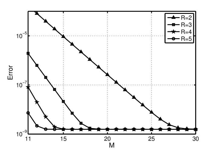
Figure 1: Error $E$ in logarithmic scale as a function of $M$ for different values of $R$ and for $N=10$

$\vartriangleright$ Spatial discretization: Computations have been carried out for ${\mathbf{u}}_{N,h}$ defined in (27) with $N=1$ and for ${\mathbf{u}}_{N,M,h}$ defined in (28) with $R=5$, $N=10$ and $M=11$ so that $e$ is in the range of $10^{-9}$ and is negligible compared to $E$. The approximation (28) is obtained from the formula (22) by substituting $\Phi_{U}$ and $\Phi_{Z}$ by the identity operator and by using the centered finite difference scheme of the second order derivative, i.e. by replacing $\Lambda$ by its discretization $\Lambda_{h}$. The spatial discretizations are compared to the expression of the approximations ${\mathbf{u}}_{N}(t,x)$ and ${\mathbf{u}}_{N,M}(t,x)$ that we calculate thanks to the modal decomposition of the operator $\partial_{xx}^{2}$ with homogeneous Dirichlet boundary conditions. It comes

$${\mathbf{u}}_{N}(t,x)=-\sum\limits_{i\in\mathbb{N}^{\ast}}w_{i}e^{-\left(\lambda_{i}^{-1}+p_{N}\left(\lambda_{i}\right)\right)t}p_{N}\left(\lambda_{i}\right)\phi_{i}\left(x\right),$$

where $\lambda_{i},$ $\phi_{i}$ and $w_{i}$ represent respectively the $i^{\text{th}}$ eigenvalue, the $i^{\text{th}}$ eigenvector and the $i^{\text{th}}$ modal coefficient of the initial condition. The same expression holds for ${\mathbf{u}}_{N,M}(t,x)$ after replacement of $p_{N}$ by $p_{N,M}$. Then, the errors,

$$\frac{\int_{0}^{T}\left(\sum_{i=0}^{\mathcal{N}}\left|{\mathbf{u}}_{N,i}-{\mathbf{u}}_{N}(x_{i})\right|^{2}\right)^{\frac{1}{2}}dt}{\int_{0}^{T}\left(\sum_{i=0}^{\mathcal{N}}\left|{\mathbf{u}}_{N,i}\right|^{2}\right)^{\frac{1}{2}}dt}\quad\text{and}\quad\frac{\int_{0}^{T}\left(\sum_{i=0}^{\mathcal{N}}\left|{\mathbf{u}}_{N,M,i}-{\mathbf{u}}_{N,M}(x_{i})\right|^{2}\right)^{\frac{1}{2}}dt}{\int_{0}^{T}\left(\sum_{i=0}^{\mathcal{N}}\left|{\mathbf{u}}_{N,M}(x_{i})\right|^{2}\right)^{\frac{1}{2}}dt},$$

are known to be theoretically quadratic with respect to $h$ the spatial discretization step, which is confirmed by our experiments.

7.2 Example 2: Heat equation with unbounded control operator

In this example, the control operator is internal and unbounded and the observation operator is internal and bounded. We apply the theory of Section 4 without going into much detail as for other examples. We only describe the state equation and the functional analysis framework.

7.2.1 The state equation

We keep the heat equation as the state equation with the same control space $U\subset L^{2}(\Omega)$ and the same functional $\mathcal{J}$ but the control operator is replaced by an unbounded one defined in the distribution sense by $\left\langle Bu,v\right\rangle=-\beta\int_{\Omega}u\beta_{1}.\nabla vdx$, where $\beta_{1}$ is a vector of $\mathbb{R}^{d}.$

7.2.2 The functional framework

First, we pose $V=H_{0}^{1}(\Omega)$, so $A=\Delta$ is an isomorphism from $V$ into $V^{\prime}$ from which we define $J=(-A)^{-1}$. It allows to give a precise definition of $B$: for all $v\in V$, $\left\langle Bu,v\right\rangle_{V^{\prime},V}=-\int_{\Omega}u\beta_{1}.\nabla v~{}dx$ for $u\in U$. Let us compute $B^{\ast}$ defined by $\left(Bu,v\right)_{V^{\prime}}=\left(u,B^{\ast}v\right)_{L^{2}(\Omega)}$ for $u\in U$ and $v\in V^{\prime}$. Since $\left(Bu,v\right)_{V^{\prime}}=\left\langle Bu,Jv\right\rangle_{V^{\prime},V}=-\left(u,\beta_{1}.\nabla Jv\right)_{L^{2}(\Omega)}$ then $B^{\ast}v=-\beta_{1}\nabla Jv$. We introduce the kernel of $B$, $K_{B}=\{u\in L^{2}\left(\Omega\right)|u$ constant in the direction$~{}\beta_{1}\},$ $U=L^{2}(\Omega)/K_{B}$ and the kernel of $B^{\ast}$, $K_{B^{\ast}}=\{v\in V^{\prime}~{}|~{}Jv~{}$constant in the direction$~{}\beta_{1}\}$. Since $Jv=0$ on the boundary $\partial\Omega$ then $K_{B^{\ast}}=\{0\}$. Then by using classical arguments, e.g. [10], one deduces that $B$ is an isomorphism from $U$ into $V^{\prime}.$ We pose also $Y=Z=L^{2}(\Omega),$ $S=C=I\in\mathcal{L}(Z,Y).$ Now, we introduce $X=V^{\prime},$ and $\Lambda=J$ which is a nonnegative operator. The fact that $\Lambda$ is self-adjoint, i.e. that $(\Lambda v,v^{\prime})_{V^{\prime}}=(v,\Lambda v^{\prime})_{V^{\prime}}$, comes from the equality $\left\langle\Lambda v,Jv^{\prime}\right\rangle_{V^{\prime},V}=\left\langle Jv,\Lambda v^{\prime}\right\rangle_{V,V^{\prime}}.$ To complete the construction, we pose $\Phi_{U}=(\beta_{1}.\nabla)^{-1},\Phi_{V}=\Lambda,\Phi_{V^{\prime}}=I,\Phi_{Y}=\Phi_{Z}=\Lambda^{1/2}$ which is an isomorphism from $V^{\prime}$ into $L^{2}(\Omega)$, $a(\Lambda)=I,\text{ }b(\Lambda)=I\text{ and }c(\Lambda)=I$. Finally, we proceed as in the first example for the computation of $p_{N,M}$.

7.3 Example 3: Beam or plate model

Here, we deal with a second order problem in time with distributed internal bounded observation and control.

7.3.1 The state equation and a choice of semi-decentralized controllers

The model under consideration is a fourth order equation posed in a domain $\Omega\subset\mathbb{R}^{d}$ which may correspond to a Euler-Bernoulli clamped beam equation when $d=1$ or to a Love-Kirchhoff clamped plate equation when $d=2$. The control is still distributed over the whole domain and the state is $z:=\begin{bmatrix}w&\partial_{t}w\end{bmatrix}^{T}$ where $w$ is solution to the boundary value problem

$$\partial_{tt}^{2}w = -\Delta^{2}w+\beta u\text{ in }\mathbb{R}^{+\ast}\times\Omega,$$ (33)

$$w = \nabla w.\nu=0\text{ on }\mathbb{R}^{+\ast}\times\partial\Omega,$$ (34)

$$w = w_{0}\text{ and }\partial_{t}w=w_{1}\text{ in }\Omega\text{ at }t=0,$$ (35)

for a given function $\beta$ and given initial conditions $w_{0}$ and $w_{1}$ all defined in $\Omega.$ Choosing the cost functional $\mathcal{J}\left(w_{0},w_{1};u\right)=\int_{0}^{+\infty}\left\|\Delta w\right\|_{L^{2}\left(\Omega\right)}^{2}+\left\|\gamma u\right\|_{L^{2}\left(\Omega\right)}^{2}dt$, we pose $\Lambda=\left(\Delta^{2}\right)^{-1},$ defined as the inverse of the biharmonic operator $\Delta^{2}:H_{0}^{2}(\Omega)\cap H^{4}(\Omega)\rightarrow L^{2}(\Omega)$. The method can handle the general case, however in the special case $\gamma=\beta=1$, we show in the following Section that the optimal control ${\mathbf{u}}$ may be approached by

$${\mathbf{u}}_{N,M,h}=-\frac{1}{2\pi}\sum_{\ell=1}^{M}\omega_{\ell}({\mathbf{v}}_{1,h}^{\ell}+\overline{{\mathbf{v}}}_{1,h}^{\ell}),$$ (36)

where $({\mathbf{v}}_{1,h}^{\ell},\overline{{\mathbf{v}}}_{1,h}^{\ell})$ are solution to

$$\begin{bmatrix}\xi_{1}-\Lambda_{h}&-\xi_{2}\\ \xi_{2}&\xi_{1}-\Lambda_{h}\end{bmatrix}\begin{bmatrix}{\mathbf{v}}_{1,h}^{\ell}\\ {\mathbf{v}}_{2,h}^{\ell}\end{bmatrix} =\begin{bmatrix}\Re e\left(-i\xi^{\prime}k_{1,N}\left(\xi\right)\right)w_{h}\\ \Im m\left(-i\xi^{\prime}k_{1,N}\left(\xi\right)\right)w_{h}\end{bmatrix},$$ (37)

$$\begin{bmatrix}\xi_{1}-\Lambda_{h}&-\xi_{2}\\ \xi_{2}&\xi_{1}-\Lambda_{h}\end{bmatrix}\begin{bmatrix}\overline{{\mathbf{v}}}_{1,h}^{\ell}\\ \overline{{\mathbf{v}}}_{2,h}^{\ell}\end{bmatrix} =\begin{bmatrix}\Re e\left(-i\xi^{\prime}k_{2,N}\left(\xi\right)\right)\partial_{t}w_{h}\\ \Im m\left(-i\xi^{\prime}k_{2,N}\left(\xi\right)\right)\partial_{t}w_{h}\end{bmatrix},$$

for each quadrature point $\xi_{\ell}:=\xi_{1,\ell}+i\xi_{2,\ell}$, and

$$\Lambda_{h}^{-1}=\dfrac{1}{h^{4}}\begin{bmatrix}2h^{3}&-\frac{1}{2}h^{3}&&&&&\\ -4&6&-4&1&&&\\ 1&\ddots&6&\ddots&\ddots&&\\ &\ddots&\ddots&\ddots&\ddots&\ddots&\\ &&\ddots&\ddots&6&\ddots&1\\ &&&1&-4&6&-4\\ &&&&&-\frac{1}{2}h^{3}&2h^{3}\end{bmatrix},$$ (38)

the vectors ${\mathbf{v}}_{i,h}^{T}$, $\overline{{\mathbf{v}}}_{i,h}^{T}$, $w_{h}^{T}$, $\partial_{t}w_{h}^{T}$ being the approximations of $\left[\begin{smallmatrix}{\mathbf{v}}_{i}(x_{1})&\ldots&{\mathbf{v}}_{i}(x_{\mathcal{N}-1})\end{smallmatrix}\right]$, $\left[\begin{smallmatrix}\overline{{\mathbf{v}}}_{i}(x_{1})&\ldots&\overline{{\mathbf{v}}}_{i}(x_{\mathcal{N}-1})\end{smallmatrix}\right]$, $\left[\begin{smallmatrix}w(x_{1})&\ldots&w(x_{\mathcal{N}-1})\end{smallmatrix}\right]$, $\left[\begin{smallmatrix}\partial_{t}w(x_{1})&\ldots&\partial_{t}w(x_{\mathcal{N}-1})\end{smallmatrix}\right]$ and $k_{i,N}$ being defined in the following section.

7.3.2 Construction and study of the semi-decentralized controllers

Firstly, the plate equation must be formulated under the form of a first order system. We set $z^{T}=\begin{bmatrix}w&\partial_{t}w\end{bmatrix}$, so we find that $A=\begin{bmatrix}0&I\\ -\Delta^{2}&0\end{bmatrix}$, the operators $B^{T}=\begin{bmatrix}0&I\end{bmatrix}$, $C=\begin{bmatrix}\Delta&0\end{bmatrix},\text{ }S=I$ and the functional spaces $U=L^{2}\left(\Omega\right)$, $Y\subset L^{2}\left(\Omega\right)$. The usual state space is $Z=H_{0}^{2}\left(\Omega\right)\times L^{2}\left(\Omega\right)$ thus $B$ and $C$ are bounded. We pose $X=L^{2}\left(\Omega\right)$, $\Lambda=\left(\Delta^{2}\right)^{-1}$ an isomorphism from $X$ into $H^{4}\left(\Omega\right)\cap H_{0}^{2}\left(\Omega\right)$, $\Phi_{Z}=\begin{bmatrix}\Lambda^{\frac{1}{2}}&0\\ 0&I\end{bmatrix}$, $\Phi_{U}=I$ and $\Phi_{Y}=\Delta\Lambda^{1/2}$, so $Y=\Delta\Lambda^{\frac{1}{2}}L^{2}\left(\Omega\right)=\Delta H_{0}^{2}\left(\Omega\right)$ and $a\left(\lambda\right)=\begin{bmatrix}0&\lambda^{-1/2}\\ -\lambda^{-1/2}&0\end{bmatrix}$, $b^{T}\left(\lambda\right)=\begin{bmatrix}0&1\end{bmatrix}$, $c\left(\lambda\right)=\begin{bmatrix}1&0\end{bmatrix}$ and $s\left(\lambda\right)=1.$

Remark 7.1.

1. We indicate how isomorphisms $\Phi_{Y}$ and $\Phi_{Z}$ have been chosen. The choice of $\Phi_{Z}$ directly comes from the expression of the inner product $\left(z,z^{\prime}\right)_{Z}=\left(\Phi_{Z}^{-1}z,\Phi_{Z}^{-1}z^{\prime}\right)_{X^{2}}$ and from $\left(z_{1},z_{1}^{\prime}\right)_{H_{0}^{2}\left(\Omega\right)}=\left(\left(\Delta^{2}\right)^{\frac{1}{2}}z_{1},\left(\Delta^{2}\right)^{\frac{1}{2}}z_{1}^{\prime}\right)_{L^{2}\left(\Omega\right)}$. For $\Phi_{Y}$, we start from $C=\Phi_{Y}c(\Lambda)\Phi_{Z}^{-1}$ and from the relation $\left(y,y^{\prime}\right)_{Y}=\left(\Phi_{Y}^{-1}y,\Phi_{Y}^{-1}y^{\prime}\right)_{X}$ which imply that $\Delta=\Phi_{Y}c_{1}\Lambda^{-\frac{1}{2}}$. The expression of $\Phi_{Y}$ follows.

2. The isomorphisms $\Phi_{Z}$ and $\Phi_{U}$ are some matrices of functions of $\Lambda$, and so $Q$ is also. Thus, the approximation is directly developed on $Q=k(\Lambda)$.

The controller $Q$ is a $1\times 2$ matrix of operators $k=\begin{bmatrix}k_{1}&k_{2}\end{bmatrix}$, with $k_{1}=p_{21}\Lambda^{-\frac{1}{2}}$ and $k_{2}=p_{22}$. So $\left(k_{i}\right)_{i=1,2}$ is solution to the system

$$\lambda k_{1}^{2}+2k_{1}-1=0\quad\text{and}\quad 2k_{1}-k_{2}^{2}=0.$$ (39)

As in the first example, a nonnegative exact solution

$$k_{1}(\lambda)=\frac{-1+\sqrt{1+\lambda}}{\lambda}\quad\text{and}\quad k_{2}(\lambda)=\sqrt{2\frac{-1+\sqrt{1+\lambda}}{\lambda}}$$

can be exhibited, so it is used to discuss numerical validation. Again, the functions $k_{i}(\lambda)$ are sufficiently regular to be accurately approximated by polynomials which computation is done using the spectral method with Legendre polynomials and the LGL quadrature formulae. The weak formulation equivalent to (39) is

$$\int_{I_{\sigma}}\left(\lambda k_{1}^{2}+2k_{1}-1\right)\eta_{1}(\lambda)\text{ }d\lambda=0\quad\text{and}\quad\int_{I_{\sigma}}\left(2k_{1}-k_{2}^{2}\right)\eta_{2}(\lambda)\text{ }d\lambda=0$$ (40)

for all $\eta_{1},$ $\eta_{2}\in\mathcal{C}^{0}\left(I_{\sigma}\right),$ it is solved by the semi-implicit Algorithm 2 below.

Algorithm 2 Semi-Implicit scheme for (40)

1:  $k_{1,N_{1}}^{0}$, $k_{2,N_{2}}^{0}$ are given.

2:  $(m+1)^{\text{th}}$ step: Knowing $(k_{1,N_{1}}^{m},k_{2,N_{2}}^{m})\in\mathbb{P}_{N_{1}}\times\mathbb{P}_{N_{2}}$, find $(k_{1,N_{1}}^{m+1},k_{2,N_{2}}^{m+1})\in\mathbb{P}_{N_{1}}\times\mathbb{P}_{N_{2}}$ such that $\forall\left(\eta_{1},\eta_{2}\right)\in\mathbb{P}_{N_{1}}\times\mathbb{P}_{N_{2}}$,

$$\int_{I_{\sigma}}k_{1,N_{1}}^{m+1}\left(\lambda\right)\left(\lambda k_{1,N_{1}}^{m}\left(\lambda\right)+2\right)\mathit{\eta}_{1}\left(\lambda\right)d\lambda=\int_{I_{\sigma}}\eta_{1}\left(\lambda\right)d\lambda,$$

$$\int_{I_{\sigma}}k_{2,N_{2}}^{m+1}\left(\lambda\right)\left(k_{2,N_{2}}^{m}\left(\lambda\right)+1\right)\eta_{2}\left(\lambda\right)d\lambda=\int_{I_{\sigma}}\left(2k_{1,N_{1}}^{m+1}\left(\lambda\right)+k_{2,N_{2}}^{m}\left(\lambda\right)\right)\eta_{2}\left(\lambda\right)d\lambda.$$

3:  If $\|k_{i,N_{i}}^{m+1}-k_{i,N_{i}}^{m}\|_{L^{2}\left(I_{\sigma}\right)}\leq\varepsilon_{i}$ then terminate the algorithm else return to Step 2

7.3.3 Numerical results

The simulations are conducted for a Euler-Bernoulli beam model with length $L=4.73m$ so that all eigenvalues of $\Lambda$ are included in $I_{\sigma}=\left(0,1\right)$.

$\vartriangleright$ Polynomial approximation: Numerical tests show an exponential convergence of the Algorithm 2. For $N_{1}=N_{2}=10$ and for null initial conditions, the exponential decay rate is about $-1.80$ and this of the differences of successive iterates $(\left\|k_{i,N_{i}}^{m+1}-k_{i,N_{i}}^{m}\right\|_{L^{2}\left(I_{\sigma}\right)})_{i=1,2}$ is about $-1.83$. The two polynomial approximation errors

$$e_{i}=\frac{\|k_{i,N_{i}}-k_{i}\|_{L^{2}(I_{\sigma})}}{\|k_{i}\|_{L^{2}(I_{\sigma})}}$$

are in the order of $10^{-10}$ and $10^{-11}$.

$\vartriangleright$ Approximation through the Cauchy formula combined with a polynomial approximation: The numerical integrations, carried out as in the first example, yield relative errors

$$E_{i}=\frac{\|k_{i,N_{i},M}-k_{i}\|_{L^{2}(I_{\sigma})}}{\|k_{i}\|_{L^{2}(I_{\sigma})}}$$

parameterized by the number $M$ of integration nodes. They decrease exponentially with respect to $M$ as shown on Figure 2 where both $M$ are varying from $11$ to $30$. Several values of the radius $R$ have been tested showing that the convergence rate is increasing with $R$.

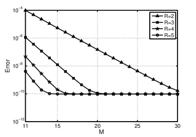
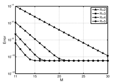
Figure 2: Relative errors 2 $E_{1}$ and 2 $E_{2}$ in logarithmic scale with respect to $M_{i}$ for different values of $R$ and for $N_{1}=N_{2}=10$

$\vartriangleright$ Spatial discretization: Taking the same notation as in Example 1, the finite difference discretization of the one-dimensional fourth order boundary value problem

$$\Delta^{2}{\mathbf{v}}=f~{}\text{in }\Omega,\quad{\mathbf{v}}=\nabla{\mathbf{v}}.\nu=0~{}\text{on }\partial\Omega,$$ (41)

is

$$\frac{1}{h^{4}}\left({\mathbf{v}}_{i-2}-4{\mathbf{v}}_{i-1}+6{\mathbf{v}}_{i}-4{\mathbf{v}}_{i+1}+{\mathbf{v}}_{i+2}\right)=f({x_{i}}),\quad\text{for }i=2,...,\mathcal{N}-2$$

for the equation in $\Omega,$ and ${\mathbf{v}}_{0}=0$, ${\mathbf{v}}_{\mathcal{N}}=0$ for the boundary conditions on ${\mathbf{v}}$. This scheme is consistant at the order 2. To do not deteriorate the error we use a second order scheme for the boundary conditions on $\partial_{x}$. From Taylor’s Theorem, ${\mathbf{v}}(x_{1})={\mathbf{v}}(0)+h\partial_{x}{\mathbf{v}}(0)+\frac{h^{2}}{2}\partial_{xx}^{2}{\mathbf{v}}(0)+\mathcal{O}\left(h^{3}\right)$ and ${\mathbf{v}}(x_{2})={\mathbf{v}}(0)+2h\partial_{x}{\mathbf{v}}(0)+2h^{2}\partial_{xx}^{2}{\mathbf{v}}(0)+\mathcal{O}\left(h^{3}\right)$. By eliminating the term in $\partial_{xx}^{2}{\mathbf{v}}(0)$ it comes $\partial_{x}{\mathbf{v}}(0)=\frac{-3{\mathbf{v}}(0)+4{\mathbf{v}}(x_{1})-{\mathbf{v}}(x_{2})}{2h}+\mathcal{O}\left(h^{2}\right)\text{.}$ The same is done for $\partial_{x}{\mathbf{v}}(L)$, we find $\partial_{x}{\mathbf{v}}(L)=\frac{-3{\mathbf{v}}(x_{\mathcal{N}})+4{\mathbf{v}}(x_{\mathcal{N}-1})-{\mathbf{v}}(x_{\mathcal{N}-2})}{2h}+\mathcal{O}\left(h^{2}\right)\text{.}$ In total, the discretization of the problem (41) after elimination of ${\mathbf{v}}_{0}$ and ${\mathbf{v}}_{\mathcal{N}}$ is written in matrix form $[\Delta_{h}^{2}]{\mathbf{v}}_{h}=f_{h},$ where ${\mathbf{v}}_{h}^{T}=\begin{bmatrix}{\mathbf{v}}_{1}&\ldots&{\mathbf{v}}_{\mathcal{N}-1}\end{bmatrix}$, $f_{h}^{T}=\begin{bmatrix}f(x_{1})&\ldots&f(x_{\mathcal{N}-1})\end{bmatrix}$ and $[\Delta_{h}^{2}]$ is the matrix in (38). The full optimal control approximation (36) is obtained by using the formulae (20-21) and the formula of ${\mathbf{u}}_{N,M,h}$ in (23) with $\Lambda_{h}=[\Delta_{h}^{2}]^{-1}$. To validate this full strategy, we have carried a computation with $R=5$, $M=11$, $10^{2}$ points in the mesh of $\Omega$ and for the time $t\in(0,T)$ with $T=15s$.

The spatial discretization is compared to the expression of the approximation ${\mathbf{u}}_{N,M}(t,x)$ that we calculate thanks to the modal decomposition of the operator $\partial_{xxxx}^{4}$ with homogeneous Dirichlet boundary conditions. Its expression is too big to be presented, it has been detailed in [25]. Denoting by ${\mathbf{u}}_{N,M,i}=\left({\mathbf{u}}_{N,M,h}\right)_{i}$ the discrete values of the control, the spatial discretization relative error

$$\frac{\int_{0}^{T}\left(\sum_{i=0}^{\mathcal{N}}\left|{\mathbf{u}}_{N,M,i}(t)-{\mathbf{u}}_{N,M}(x_{i},t)\right|^{2}\right)^{\frac{1}{2}}dt}{\int_{0}^{T}\left(\sum_{i=0}^{\mathcal{N}}\left|{\mathbf{u}}_{N,M}(x_{i},t)\right|^{2}\right)^{\frac{1}{2}}dt}$$

between $u_{N,M}$ and $u_{N,M,h}$ is equal to $1.10\times 10^{-4}$.

7.4 Example 4: Two-dimensional heat equation with a boundary control

This example deals with a special case of boundary control.

7.4.1 The state equation and a choice of semi-decentralized controller

Let $\Omega$ be the rectangle $\left(0,1\right)\times\left(0,\pi\right)\subset\mathbb{R}^{2}$ and $\Gamma_{0}=\left\{\left(0,y\right):0<y<\pi\right\}$ a part of its boundary. Let us consider the heat equation with a control $v(t,y)$ applied to the boundary $\Gamma_{0}$,

$$\left\{\begin{aligned} \partial_{t}w\left(t,x,y\right)-\partial_{xx}^{2}w\left(t,x,y\right)-\partial_{yy}^{2}w\left(t,x,y\right)&=0&&\text{in }\mathbb{R}^{+\ast}\times\Omega,\\ w\left(t,0,y\right)&=v\left(t,y\right)&&\text{on }\mathbb{R}^{+\ast}\times\Gamma_{0},\\ w\left(t,x,y\right)&=0&&\text{on }\mathbb{R}^{+\ast}\times\partial\Omega\backslash\Gamma_{0},\\ w\left(0,x,y\right)&=w_{0}\left(x,y\right)&&\text{in }\Omega\text{.}\end{aligned}\right.$$

Since our method is not directly applicable, we reduce the problem to an internal control problem. We introduce $\overline{w}\left(t,x,y\right)=w\left(t,x,y\right)-\left(1-x\right)v\left(t,y\right)$ solution to the heat equation with homogeneous boundary conditions,

$$\left\{\begin{aligned} \partial_{t}\overline{w}\left(t,x,y\right)&=\partial_{xx}^{2}\overline{w}\left(t,x,y\right)+\partial_{yy}^{2}\overline{w}\left(t,x,y\right)-\left(1-x\right)u\left(t,y\right)&&\text{in }\mathbb{R}^{+\ast}\times\Omega,\\ \overline{w}\left(t,x,y\right)&=0&&\text{on }\mathbb{R}^{+\ast}\times\partial\Omega,\\ \overline{w}\left(0,x,y\right)&=\overline{w}_{0}\left(x,y\right)=w_{0}\left(x,y\right)-\left(1-x\right)w_{0}\left(0,y\right)&&\text{in }\Omega,\end{aligned}\right.$$

with $u\left(t,y\right)=\partial_{t}v\left(t,y\right)-\partial_{yy}^{2}v\left(t,y\right)$ that allows for easy computation of $v$ once $u$ is known. For simplicity, we define the cost function and the control space with $u$ instead of $v$. So, we chose the control space $U\subset L^{2}\left(\Gamma_{0}\right)$ and the cost functional

$$\mathcal{J}\left(\overline{w}_{0};u\right)=\int_{0}^{+\infty}\left\|\overline{w}\left(t,x,y\right)\right\|_{L^{2}\left(\Omega\right)}^{2}+\left\|u\left(t,y\right)\right\|_{L^{2}\left(\Gamma_{0}\right)}^{2}\text{ }dt\text{.}$$ (42)

Then, the approximation of the control is done by using $J$ terms in a modal decomposition of $\partial_{xx}^{2}$. Without entering into much details, that are given in sub-Section 7.4.2, the state vector is comprised with $J$ components $\overline{w}_{j}\left(t,y\right)=\sqrt{2}\int_{0}^{1}\overline{w}\left(t,x,y\right)\sin\left(j\pi x\right)$ $dx$ and the associated control is therefore ${\mathbf{u}}=-k(\Lambda)z$ where $k$ is a $J$-row vector of functions and $\Lambda$ is the isomorphism $(-\partial_{yy}^{2})^{-1}:L^{2}(\Gamma_{0})\rightarrow H^{2}(\Gamma_{0})\cap H_{0}^{1}(\Gamma_{0})$. A semi-decentralized control is built from a rational approximation $k_{j,N_{j}}$ of each component $k_{j}$ and from a quadrature rule in the Cauchy formula,

$${\mathbf{u}}_{N,M,h}=-\frac{1}{2\pi}\sum_{\ell=1}^{M}\omega_{\ell}\sum_{j=1}^{J}{\mathbf{v}}_{1,h}^{\ell,j},$$ (43)

where each ${\mathbf{v}}_{1,h}^{\ell,j}$ is solution to a system like (29) with $\overline{w}_{j,h}$ instead of $w_{h}$ and $k_{j,N_{j}}$ instead of $p_{N}.$

7.4.2 Construction and study of the semi-decentralized controller

We start with projecting the model on the $J$ first components of the orthonormal basis $\psi_{j}\left(x\right)=\sqrt{2}\sin\left(j\pi x\right)$ in $L^{2}(0,1)$. Since $\int_{0}^{1}\left(1-x\right)\psi_{j}(x)~{}dx=\frac{\sqrt{2}}{j\pi}$ the components $\overline{w}_{j}\left(t,y\right)$ are solution to the equations posed on $\Gamma_{0}$,

$$\left\{\begin{aligned} \partial_{t}\overline{w}_{j}\left(t,y\right)&=-j^{2}\pi^{2}\overline{w}_{j}\left(t,y\right)+\partial_{yy}^{2}\overline{w}_{j}\left(t,y\right)-\frac{\sqrt{2}}{j\pi}u\left(t,y\right)&&\text{in }\mathbb{R}^{+\ast}\times\Gamma_{0},\\ \overline{w}_{j}\left(t,0\right)&=\overline{w}_{j}\left(t,\pi\right)=0&&\text{in }\mathbb{R}^{+\ast},\\ \overline{w}_{j}\left(0,y\right)&=\overline{w}_{j,0}\left(y\right)=\int_{0}^{1}\overline{w}_{0}\left(x,y\right)\psi_{j}\left(x\right)dx&&\text{in }\Gamma_{0}\text{.}\end{aligned}\right.$$ (44)

This is the system of state equations coupled by a common internal control $u\left(t,y\right)$. The cost functional (42) is reduced to

$$\mathcal{J}\left(\overline{w}_{0};u\right)\simeq\mathcal{J}\left(\overline{w}_{.,0};u\right)=\int_{0}^{+\infty}\sum_{j=1}^{J}||\overline{w}_{j}\left(t,y\right)||_{L^{2}\left(\Gamma_{0}\right)}^{2}+||u\left(t,y\right)||_{L^{2}\left(\Gamma_{0}\right)}^{2}~{}dt.$$

Then, the state variable is $z^{T}=\begin{bmatrix}\overline{w}_{1}&\ldots&\overline{w}_{J}\end{bmatrix}$, $A=-{\rm diag}[(j^{2}\pi^{2}+\Lambda^{-1})_{j=1\ldots J}]$, $B^{T}=\frac{\sqrt{2}}{\pi}\begin{bmatrix}\frac{I}{1}&\ldots&\frac{I}{J}\end{bmatrix}$, and $C$ is the identity operator. The control and the observation spaces are $U=L^{2}\left(\Gamma_{0}\right)$ and $Y=\left(L^{2}\left(\Gamma_{0}\right)\right)^{J}$. In addition we pose $X=L^{2}\left(\Gamma_{0}\right)$ and the state space $Z=\left(L^{2}\left(\Gamma_{0}\right)\right)^{J}$ thus $B$ and $C$ are bounded. Thus $\Phi_{Z}=\Phi_{Y}=I_{J\times J}$, $\Phi_{U}=I$ and $a\left(\lambda\right)=-{\rm diag}\left[(j^{2}\pi^{2}+\frac{1}{\lambda})_{j=1\ldots J}\right]$, $b^{T}\left(\lambda\right)=\frac{\sqrt{2}}{\pi}\begin{bmatrix}\frac{1}{1}&\ldots&\frac{1}{J}\end{bmatrix}$ and $c\left(\text{.}\right)$ is the identity operator on $\mathbb{R}^{J}$. Since $\Phi_{Z}$ and $\Phi_{U}$ are the identity operators, the approximation is developed on $Q=k(\Lambda)$ with $k(\Lambda)=q(\Lambda)$, and the exact optimal control is ${\mathbf{u}}=-k(\Lambda)z$.

To build a rational interpolation $k_{N}\left(\lambda\right)$ of the form (15) the interval $I_{\sigma}=(0,1]$ is meshed with $L+1$ distinct nodes $\lambda_{0},\ldots,\lambda_{L}$ and each $p\left(\lambda_{n}\right)$ solutions to the ARE is accurately computed with a standard solver. The exact expression of $k\left(\lambda_{n}\right)=b^{T}p\left(\lambda_{n}\right)$ follows and the coefficients of the rational approximation are solution to the $L+1$ equations $k_{j,N_{j}}\left(\lambda_{n}\right)=k_{j}\left(\lambda_{n}\right)$ i.e. to

$$\sum\limits_{m=0}^{N_{j}^{N}}d_{m}\lambda_{n}^{m}-k_{j}\left(\lambda_{n}\right)\sum_{m^{\prime}=0}^{N_{j}^{D}}d_{m^{\prime}}^{\prime}\lambda_{n}^{m^{\prime}}=0\text{ for }n=0,\ldots,L.$$

The number $L$ of equations is taken sufficiently large so that the system with $N^{N}+N^{D}+2$ unknowns is over-determined and is solved in the mean square sense by using the singular value decomposition.

7.4.3 Numerical results

The simulation have been conducted with four modes i.e. for $J=4$. The shape of the four first functions $k_{j}(\lambda)$ are represented in Figure 3 which shows that they exhibit a singular behavior at the origin. Thus, they can not be accurately approximated by polynomials but may be by rational functions.

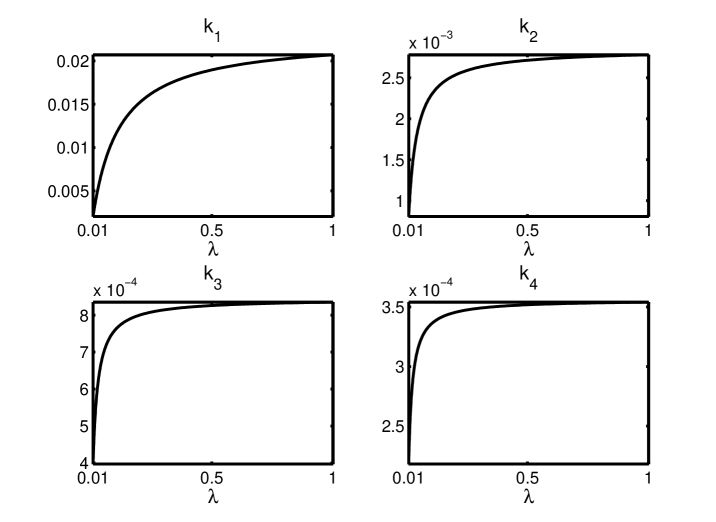
Figure 3: Shapes of the Spectral Functions $k$

$\vartriangleright$ Rational approximation: In order to get an accurate approximation, we choose a logarithmic distribution of $100$ nodes in $(10^{-2},1)$, which corresponds to a truncation of high frequencies. In Table 1, we report the relative errors in the discrete $\ell^{2}$-norm on the other set $\{\lambda_{n}\}_{n=0\ldots 200}$

$$e_{j}=\frac{\left(\sum_{n=0}^{200}\left|k_{j,N_{j}}\left(\lambda_{n}\right)-k_{j}\left(\lambda_{n}\right)\right|^{2}\right)^{\frac{1}{2}}}{\left(\sum_{n=0}^{200}\left|k_{j}\left(\lambda_{n}\right)\right|^{2}\right)^{\frac{1}{2}}},\text{ with }\lambda_{n}=10^{-2+\frac{n}{100}}\quad\text{for }j=1,\ldots,4,$$

between the exact function $k_{j}$ and its rational approximation $k_{j,N_{j}}$ for special values of numerator’s and denominator’s polynomial degrees $N_{j}=\left(N_{j}^{N},N_{j}^{D}\right)$

Table 1: Errors of the rational approximations with numerator’s and denominator’s degrees $N_{j}=\left(N_{j}^{N},N_{j}^{D}\right)$

$j$	$1$	$2$	$3$	$4$
$N_{j}$	$\left(19,3\right)$	$\left(18,3\right)$	$\left(17,1\right)$	$\left(20,2\right)$
$e_{j}\times 10^{-10}$	$0.003$	$0.013$	$1.003$	$0.182$

$\vartriangleright$ The Cauchy formula combined with rational approximations: Then, according to Remark 6.3, numerical integrations are performed with a standard trapezoidal quadrature rule along the ellipse defined by the two radii in the real and imaginary directions $R_{1}=1.02$ and $R_{2}=0.07$. The relative errors

$$E_{j}=\frac{\left(\sum_{n=0}^{200}\left|k_{j,N_{j},M}\left(\lambda_{n}\right)-k_{j}\left(\lambda_{n}\right)\right|^{2}\right)^{\frac{1}{2}}}{\left(\sum_{n=0}^{200}\left|k_{j}\left(\lambda_{n}\right)\right|^{2}\right)^{\frac{1}{2}}}\text{ with }\lambda_{n}=10^{-2+\frac{n}{100}}\quad\text{for }j=1,\ldots,4,$$

between the exact functions and final approximations are plotted in logarithmic scale in Figure 4 for $M$ varying from $10$ to $5\times 10^{2}$. The errors converge exponentially with an exponential decay rate given in Figure 4. Note that the parameters $R_{1}$ and $R_{2}$ of the ellipse affects the rate of convergence errors, which is confirmed by our numerical calculation.

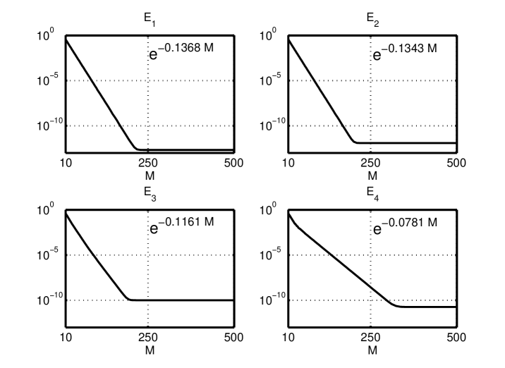
Figure 4: Errors between $k$ and $k_{N,M}$

$\vartriangleright$ Spatial discretization: The approximation (43) is obtained from the formula of ${\mathbf{u}}_{N,M,h}$ in (23) and by using the centered finite difference scheme of the second order derivative $\partial_{yy}^{2}$. The expression of $\Lambda_{h}$ is the same as in Example 1 and the error between ${\mathbf{u}}_{N,M,h}$ and ${\mathbf{u}}$ is quadratic in the space step $h$.

8 Conclusion

We have proposed a method to compute distributed control applied to linear distributed systems with a control operator that is bounded or not. It has been conceived for architectures of semi-decentralized processors. Its construction uses a functional calculus for matrices of functions of an operator, based on spectral theory and Cauchy formula. In the case of polynomial approximation of $k$, we have noticed that the numerical integration needs few integration points, and that the radius of the contour affects the accuracy of the numerical integration of the Cauchy formula. If the approximation is rational, we have concluded that numerical integration requires more integration points in the ellipse which parameters have been chosen heuristically. We think that the performance of the method could be further improved by finding optimal contour parameters depending on the number of quadrature nodes following the ideas in J. A. C. Weideman and L. N. Trefethen [24]. Finally, the method can be extended to other frameworks for distributed control and for functional calculus.

References

• [1] B. Bamieh, F. Paganini, and M.A. Dahleh. Distributed control of spatially invariant systems. IEEE Transactions on Automatic Control, 47(7):1091–107, 2002.
• [2] H. T. Banks and K. Ito. Approximation in lqr problems for infinite-dimensional systems with unbounded input operators. J. Math. Systems Estim. Control, 7(1):p. 34 pp., 1997.
• [3] C. Bernardi and Y. Maday. Some spectral approximations of one-dimensional fourth-order problems, in: P. nevai and a. pinkus, eds. In Progress in approximation theory, page 43116, 1991.
• [4] C. Bernardi and Y. Maday. Approximations spectrales de problèmes aux limites elliptiques. Mathematiques et Applications 10. Springer-Verlag, (1992).
• [5] M. Crouzeix and A. L. Mignot. Analyse numérique des équations différentielles. Collection Mathématiques Appliquées pour la Maitrise. Masson, Paris, 1984.
• [6] R. F. Curtain and H. Zwart. An introduction to infinite-dimensional linear systems theory, volume 21 of Texts in Applied Mathematics. Springer-Verlag, 1995.
• [7] R. D’Andrea and G. E. Dullerud. Distributed control design for spatially interconnected systems. IEEE Trans. Automat. Control, 48(9):1478–1495, 2003.
• [8] R. Dautray and J.-L. Lions. Mathematical analysis and numerical methods for science and technology, volume 3. Springer-Verlag, Berlin, 1990.
• [9] P. J. Davis and P. Rabinowitz. Methods of Numerical Integration. Computer Science and Applied Mathematics. Academic Press Inc., Orlando, FL,, edition, 1984.
• [10] V. Girault and P.-A. Raviart. Finite element methods for Navier-Stokes equations, volume 5 of Springer Series in Computational Mathematics. Springer-Verlag, Berlin, 1986. theory and algorithms.
• [11] P. Grisvard. Elliptic problems in nonsmooth domains, volume 24 of Monographs and Studies in Mathematics. Pitman Advanced Publications Program, Boston-London-Melbourne, 1985. theory and algorithms.
• [12] M. Haase. The functional calculus for sectorial operators, volume 169 of Operator Theory: Advances and Applications. Birkh user Verlag, Boston, 2006.
• [13] H. Hui, Y. Yakoubi, M. Lenczner, and Ratier. Semi-decentralized approximation of a lqr-based controller for a one-dimensional cantilever array. 18th IFAC World Congress, August 28 - September 2, 2011, Milano, Italy.
• [14] M. R. Jovanović. On the optimality of localized distributed controllers. Int. J. Systems, Control and Communications, 2(1/2/3):82–99, 2010.
• [15] M. Kader, M. Lenczner, and Z. Mrcarica. Approximation of an optimal control law using a distributed electronic circuit: application to vibration control. Comptes Rendus de l’Academie des Sciences Serie II b/Mecanique, 328(7):547 – 53, 2000.
• [16] C. Langbort and R. D’Andrea. Distributed control of spatially reversible interconnected systems with boundary conditions. SIAM J. Control Optim., 44(1):1–28, 2005.
• [17] I. Lasiecka and R. Triggiani. Control theory for partial differential equations: continuous and approximation theories. I, volume 74 of Encyclopedia of Mathematics and its Applications. Birkhäuser Verlag, 2000.
• [18] M. Lenczner, G. Montseny, and Y. Yakoubi. Diffusive realizations for solutions of some operator equations. Math. Comput., 81(277):319–344, 2012.
• [19] M. Lenczner and Y. Yakoubi. Semi-decentralized approximation of optimal control for partial differential equations in bounded domains. Comptes Rendus Mécanique, 337(4):245–250, 2009.
• [20] J.-L. Lions. Optimal control of systems governed by partial differential equations. Die Grundlehren der mathematischen Wissenschaften, Band 170. Springer-Verlag, 1971.
• [21] C. Martinez Carracedo and M. Sanz Alix. The theory of fractional powers of operators, volume 187 of North-Holland Mathematics Studies. North-Holland Publishing Co., 2001.
• [22] F. Paganini and B. Bamieh. Decentralization properties of optimal distributed controllers. Proceedings of the IEEE Conference on Decision and Control, 2:1877–1882, 1998.
• [23] J. Sanchez Hubert and E. Sanchez-Palencia. Vibration and coupling of continuous systems: asymptotic methods. Springer-Verlag, 1989.
• [24] J. A. C. Weideman and L. N. Trefethen. Parabolic and hyperbolic contours for computing the bromwich integral. Math. Comp., 76(259):1341–1356, 2007.
• [25] Y. Yakoubi. Two approximation methods for semi-decentralized optimal control of distributed systems. PhD Thesis, University de Franche-Comté, July 15th 2010.
• [26] K. Yosida. Functional analysis. Classics in Mathematics. Springer-Verlag, 1995. Reprint of the sixth (1980) edition.