A microscopic model for detecting the surface states photoelectrons in Topological Insulators
D.Schmeltzer
Physics Department, City College of the City University of New York
New York, New York 10031
Abstract
We present a model for the photoelectrons emitted from the surface of a Topological insulator induced by a polarized laser source. The model is based on the tunneling of the surface electrons into the vacuum in the presence of a photon field. Using the Hamiltonian which describes the coupling of the photons to the surface electrons we compute the intensity and polarization of the photoelectrons.
Recently the use of an innovative spectrometer with a high laser-based light source have shown that the spin polarization of the photoelectrons emitted from the surface of the B β i 2 β S β e 3 π΅ subscript π 2 π subscript π 3 Bi_{2}Se_{3} Topological Insulator (T . I . formulae-sequence π πΌ T.I. ) Volkov ; Zhang ; Kane ; David can be manipulated through the laser light polarization Nature . One finds that the photoelectrons polarization is completely different from the initial states and is controlled by the photon polarization. A number of theories have been proposed Park ; Wang ; Moore .
A correct theory for this effect is important since the photoemission experiments are used to investigate the nature of the surface states.
The theory given by Park suggest that the photoelectron current with the spin part in the t ^ ^ π‘ \hat{t} direction is given by S β β
t ^ β
β π ^ π‘ \vec{S}\cdot\hat{t} where S β β π \vec{S} is the spin polarization of the photoelectrons. The state recorded by the photodetector at position R β d subscript β π
π \vec{R}_{d} is given by | t ^ , R β d > ket ^ π‘ subscript β π
π
|\hat{t},\vec{R}_{d}> . The photocurrent induced from the intial T.I. state | i > ket π |i> depends on the photoexcited states | f > ket π |f> of the Topological Surface States. (T . S . S . formulae-sequence π π π T.S.S. ) is given in ref. Park :
I t ^ β | β E f = E i + β β Ξ© < t ^ , , R β d | f > < f | H i β n β t | i > | 2 I_{\hat{t}}\propto|\sum_{E_{f}=E_{i}+\hbar\Omega}<\hat{t},,\vec{R}_{d}|f><f|H^{int}|i>|^{2} where H i β n β t superscript π» π π π‘ H^{int} is the matrix element between the initial surface electron and final state and β¨ t ^ , R β d | f β© inner-product ^ π‘ subscript β π
π
π \langle\hat{t},\vec{R}_{d}|f\rangle is the projection of the final state | f β© ket π |f\rangle measured by the detector.
This phenomenological description is based the Fermi Golden rule for the photoemission cross section.
Recently it has been suggested Lin that interactions and hybridization between the bands in a T.I. might be responsible for the modification of the photoemission spectrum.
The purpose of this paper is to present a microscopic model which explains the photoemission experimental results. We present a model where the surface T . I . formulae-sequence π πΌ T.I. conduction band are coupled to the normal electrons of the vacuum states. Such a model emerges when we consider the bulk T . I . formulae-sequence π πΌ T.I. electrons which give rise to the surface states , the surface states have a non-zero amplitude to tunnel into the vacuum Fan ; David .
The basic T . S . S . formulae-sequence π π π T.S.S. Hamiltonian in the presence of the vector potential A β β π΄ \vec{A} is given by the Weyl model D.S. :
H = β β v β β« d 2 β r β Ξ¨ β β ( r β ) β [ Ο 1 β ( β i β β 2 β e β β A 2 β ( r β , t ) ) β Ο 2 β ( β i β β 1 β e β β A 1 β ( r β , t ) ) ] β Ξ¨ β ( r β ) , π» Planck-constant-over-2-pi π£ superscript π 2 π superscript Ξ¨ β β π delimited-[] superscript π 1 π subscript 2 π Planck-constant-over-2-pi subscript π΄ 2 β π π‘ superscript π 2 π subscript 1 π Planck-constant-over-2-pi subscript π΄ 1 β π π‘ Ξ¨ β π \displaystyle H=\hbar v\int\,d^{2}r\Psi^{\dagger}(\vec{r})\left[\sigma^{1}\left(-i\partial_{2}-\frac{e}{\hbar}A_{2}(\vec{r},t)\right)-\sigma^{2}\left(-i\partial_{1}-\frac{e}{\hbar}A_{1}(\vec{r},t)\right)\right]\Psi(\vec{r}),
The spinor operator Ξ¨ β ( r β ) Ξ¨ β π \Psi(\vec{r}) is decomposed into the eigenvalues of the unperturbed Weyl Hamiltonian
Ξ¨ β ( r β ) = v β β k β e i β k β β
r β β [ C β ( k β ) β u ( + ) β ( k β ) + B β β ( β k β ) β u ( β ) β ( β k β ) ] β‘ v β β k β e i β k β β
r β β Ξ¨ β ( k β ) . Ξ¨ β π π£ subscript β π superscript π β
π β π β π delimited-[] πΆ β π superscript π’ β π superscript π΅ β β π superscript π’ β π π£ subscript β π superscript π β
π β π β π Ξ¨ β π \Psi(\vec{r})=\sqrt{v}\sum_{\vec{k}}e^{i\vec{k}\cdot\vec{r}}[C(\vec{k})u^{(+)}(\vec{k})+B^{\dagger}(-\vec{k})u^{(-)}(-\vec{k})]\equiv\sqrt{v}\sum_{\vec{k}}e^{i\vec{k}\cdot\vec{r}}\Psi(\vec{k}).
(2)
where | u ( + ) β ( k β ) β© ket superscript π’ β π |u^{(+)}(\vec{k})\rangle is the eigenvector for particles (positive energies) and | u ( β ) β ( k β ) β© ket superscript π’ β π |u^{(-)}(\vec{k})\rangle is the spinor for antiparticles (negative energies) :
| u ( β ) β ( k β ) β© = 1 2 β [ | k β β© β [ i β e β i β Ο β ( k β ) , 1 ] T ] . , ket superscript π’ β π 1 2 delimited-[] tensor-product ket β π superscript π superscript π π π β π 1 π \displaystyle|u^{(-)}(\vec{k})\rangle=\frac{1}{\sqrt{2}}\Big{[}|\vec{k}\rangle\otimes[ie^{-i\chi(\vec{k})},1]^{T}\Big{]}.,
| u ( + ) β ( k β ) β© = 1 2 β [ | k β β© β [ 1 , β i β e i β Ο β ( k β ) ] T ] , . ket superscript π’ β π 1 2 delimited-[] tensor-product ket β π superscript 1 π superscript π π π β π π \displaystyle|u^{(+)}(\vec{k})\rangle=\frac{1}{\sqrt{2}}\Big{[}|\vec{k}\rangle\otimes[1,-ie^{i\chi(\vec{k})}]^{T}\Big{]},\hskip 14.45377pt.
(3)
The eigenvectors are given in terms of the multivalued phase Ο β ( k β ) π β π \chi(\vec{k}) , tan β‘ ( Ο β ( k β ) ) = k 2 k 1 π β π subscript π 2 subscript π 1 \tan(\chi(\vec{k}))=\frac{k_{2}}{k_{1}} .
We choose for the particle operators C β ( k β ) πΆ β π C(\vec{k}) , C β β ( k β ) superscript πΆ β β π C^{\dagger}(\vec{k}) and for the anti-particles the operators B β ( k β ) π΅ β π B(\vec{k}) , B β β ( k β ) superscript π΅ β β π B^{\dagger}(\vec{k}) .
In order to construct the explicit model we will take the chemical potential ΞΌ = 0.3 π 0.3 \mu=0.3 ev.
We can consider only the particle band, electrons excitations above the Dirac Cone.The momentum k β β π \vec{k} is the momentum parallel to the surface located at z = 0 π§ 0 z=0 . For simplicity we have ignored the hexagonal warping effect on the energy spectrum of the quasi-particles Liang and consider only the effect on the spinors D.S. .
Next we present the three parts of the model : A- the one band Hamiltonian and the coupling to the photon field ; B-The coupling of the surface electrons to the vacuum electrons ; C-The spin detection Hamiltonian:
A- The one band Hamiltonian and the coupling to the external photon field is given by :
H ( c ) = β k β ( β β v β | k β | β ΞΌ ) β C β β ( k β , z = 0 ) β C β ( k β , z = 0 ) superscript π» π subscript β π Planck-constant-over-2-pi π£ β π π superscript πΆ β β π π§
0 πΆ β π π§
0 H^{(c)}=\sum_{\vec{k}}(\hbar v|\vec{k}|-\mu)C^{\dagger}(\vec{k},z=0)C(\vec{k},z=0)
(4)
The Hamiltonian H ( c ) superscript π» π H^{(c)} with the chemical potential ΞΌ π \mu describe the surface conduction electrons localized on the surface z = 0 π§ 0 z=0 . In agreement with ref. D.S. we only consider the conduction electrons and ignore the antiparticles excitations.
The coupling to the photon field is given according to ref.D.S. and depends explicitly on the matrix elements β¨ u ( + ) β ( k β ) | Ο 1 | u ( + ) β ( p β ) β© quantum-operator-product superscript π’ β π superscript π 1 superscript π’ β π \langle u^{(+)}(\vec{k})|\sigma^{1}|u^{(+)}(\vec{p})\rangle and β¨ u ( + ) β ( k β ) | β Ο 2 | u ( + ) β ( p β ) β© quantum-operator-product superscript π’ β π superscript π 2 superscript π’ β π \langle u^{(+)}(\vec{k})|-\sigma^{2}|u^{(+)}(\vec{p})\rangle .
H e β x β t β ( t ) = β« d 2 β r β [ J 1 β ( r β , t ) β A 1 β ( r β , t ) + J 2 β ( r β , t ) β A 2 β ( r β , t ) ] = ( β e β v ) β β« d 2 β k ( 2 β Ο ) 2 β β« d 2 β p ( 2 β Ο ) 2 superscript π» π π₯ π‘ π‘ superscript π 2 π delimited-[] subscript π½ 1 β π π‘ subscript π΄ 1 β π π‘ subscript π½ 2 β π π‘ subscript π΄ 2 β π π‘ π π£ superscript π 2 π superscript 2 π 2 superscript π 2 π superscript 2 π 2 \displaystyle H^{ext}(t)=\int\ d^{2}r[J_{1}(\vec{r},t)A_{1}(\vec{r},t)+J_{2}(\vec{r},t)A_{2}(\vec{r},t)]=(-ev)\int\frac{d^{2}k}{(2\pi)^{2}}\int\frac{d^{2}p}{(2\pi)^{2}}
C β β ( k β , t ) β C β ( p β , t ) β [ β¨ u ( + ) β ( k β ) | β Ο 2 | u ( + ) β ( p β ) β© β A 1 β ( β ( k β β p β ) , t ) + β¨ u ( + ) β ( k β ) | Ο 1 | u ( + ) β ( p β ) β© β A 2 β ( β ( k β β p β ) , t ) ] superscript πΆ β β π π‘ πΆ β π π‘ delimited-[] quantum-operator-product superscript π’ β π superscript π 2 superscript π’ β π subscript π΄ 1 β π β π π‘ quantum-operator-product superscript π’ β π superscript π 1 superscript π’ β π subscript π΄ 2 β π β π π‘ \displaystyle C^{\dagger}(\vec{k},t)C(\vec{p},t)[\langle u^{(+)}(\vec{k})|-\sigma^{2}|u^{(+)}(\vec{p})\rangle A_{1}(-(\vec{k}-\vec{p}),t)+\langle u^{(+)}(\vec{k})|\sigma^{1}|u^{(+)}(\vec{p})\rangle A_{2}(-(\vec{k}-\vec{p}),t)]
= ( β e β v ) β β« d 2 β k ( 2 β Ο ) 2 β β« d 2 β p ( 2 β Ο ) 2 β C ^ β β ( k β , t ) β C ^ β ( p β , t ) β [ W x β ( k β , p β ) β A x β ( β ( k β β p β ) , t ) + W y β ( k β , p β ) β A y β ( β ( k β β p β ) , t ) ] absent π π£ superscript π 2 π superscript 2 π 2 superscript π 2 π superscript 2 π 2 superscript ^ πΆ β β π π‘ ^ πΆ β π π‘ delimited-[] subscript π π₯ β π β π subscript π΄ π₯ β π β π π‘ subscript π π¦ β π β π subscript π΄ π¦ β π β π π‘ \displaystyle=(-ev)\int\frac{d^{2}k}{(2\pi)^{2}}\int\frac{d^{2}p}{(2\pi)^{2}}\hat{C}^{\dagger}(\vec{k},t)\hat{C}(\vec{p},t)\Big{[}W_{x}(\vec{k},\vec{p})A_{x}(-(\vec{k}-\vec{p}),t)+W_{y}(\vec{k},\vec{p})A_{y}(-(\vec{k}-\vec{p}),t)\Big{]}
W x β ( k β , p β ) = cos β‘ [ 1 2 β ( Ο β ( k β ) + Ο β ( p β ) ) ] ; W y β ( k β , p β ) = β sin β‘ [ 1 2 β ( Ο β ( k β ) + Ο β ( p β ) ) ] formulae-sequence subscript π π₯ β π β π 1 2 π β π π β π subscript π π¦ β π β π 1 2 π β π π β π \displaystyle W_{x}(\vec{k},\vec{p})=\cos[\frac{1}{2}(\chi(\vec{k})+\chi(\vec{p}))];W_{y}(\vec{k},\vec{p})=-\sin[\frac{1}{2}(\chi(\vec{k})+\chi(\vec{p}))]
The photon field A β β ( P β β‘ p β β k β , p z ) β π΄ β π β π β π subscript π π§
\vec{A}(\vec{P}\equiv\vec{p}-\vec{k},p_{z}) characterized by the coherent state | Ξ© > ket Ξ© |\Omega> . The direction of the incoming photon with respect the surface located at z = 0 π§ 0 z=0 is given by the vector P β | P β | β π β π \frac{\vec{P}}{|\vec{P}|} . The two transversal polarization are given by the vectors e β s = 1 β ( P β ) subscript β π π 1 β π \vec{e}_{s=1}(\vec{P}) and e β s = 2 β ( P β ) subscript β π π 2 β π \vec{e}_{s=2}(\vec{P}) which are perpendicular to the photon propagation.
A β ( P β , t ) = β s = 1 , 2 [ e s β ( P β ) a s ( P β ) e β i β Ξ© β t + e s β ( P β ) a s β ( P ) β e i β Ξ© β t ] \displaystyle\vec{A}(\vec{P},t)=\sum_{s=1,2}[\vec{e_{s}}(\vec{P})a_{s}(\vec{P})e^{-i\Omega t}+\vec{e_{s}}(\vec{P})a^{\dagger}_{s}(\vec{P)}e^{i\Omega t}]
P β | P β | = ( s β i β n β [ ΞΈ ] β c β o β s β [ Ο ] , s β i β n β [ ΞΈ ] β s β i β n β [ Ο ] , c β o β s β [ ΞΈ ] ) β π β π π π π delimited-[] π π π π delimited-[] italic-Ο π π π delimited-[] π π π π delimited-[] italic-Ο π π π delimited-[] π \displaystyle\frac{\vec{P}}{|\vec{P}|}=(sin[\theta]cos[\phi],sin[\theta]sin[\phi],cos[\theta])
e β s = 1 β ( P β ) = ( c β o β s β [ ΞΈ ] β c β o β s β [ Ο ] , c β o β s β [ ΞΈ ] β s β i β n β [ Ο ] , β s β i β n β [ ΞΈ ] ) subscript β π π 1 β π π π π delimited-[] π π π π delimited-[] italic-Ο π π π delimited-[] π π π π delimited-[] italic-Ο π π π delimited-[] π \displaystyle\vec{e}_{s=1}(\vec{P})=(cos[\theta]cos[\phi],cos[\theta]sin[\phi],-sin[\theta])
e β s = 2 β ( P β ) = ( β s β i β n β [ Ο ] , c β o β s β [ Ο ] , 0 ) subscript β π π 2 β π π π π delimited-[] italic-Ο π π π delimited-[] italic-Ο 0 \displaystyle\vec{e}_{s=2}(\vec{P})=(-sin[\phi],cos[\phi],0)
The coherent state condition for the photon field with the frequency Ξ© Ξ© \Omega is given by:a s β ( P β ) β | Ξ© > = a ^ s β ( P β ) β | Ξ© β© subscript π π β π ket Ξ© subscript ^ π π β π ket Ξ© a_{s}(\vec{P})|\Omega>=\hat{a}_{s}(\vec{P})|\Omega\rangle . For the remaining part the photon momentum will be neglected in comparison with the electrons quasi-momentum.
B-The hybridization between the surface electrons and emitted vacuum electrons.
We will assume that the electrons in the vacuum are described by the creation and annihilation operators b Ξ± β β ( k β , k z ) subscript superscript π β πΌ β π subscript π π§ b^{\dagger}_{\alpha}(\vec{k},k_{z}) and b Ξ± β ( k β , k z ) subscript π πΌ β π subscript π π§ b_{\alpha}(\vec{k},k_{z}) with the single particles energy,
E f β ( k β , k z ) = β 2 β K 2 2 β m + V 0 subscript πΈ π β π subscript π π§ superscript Planck-constant-over-2-pi 2 superscript πΎ 2 2 π subscript π 0 E_{f}(\vec{k},k_{z})=\frac{\hbar^{2}K^{2}}{2m}+V_{0} , where V 0 subscript π 0 V_{0} is the binding- work function for the T . S . S . formulae-sequence π π π T.S.S. surface. The tunneling Hamiltonian between the surface at z = 0 π§ 0 z=0 and the vacuum is given by:
H t z = 0 = β« d 2 β k ( 2 β Ο ) 2 β« d β k z 1 2 β Ο β« d β k z 1 2 β Ο [ t ( k z 1 , k z 2 ) C Ξ± β ( k β , k z 1 ) b Ξ± ( k β , k z 2 ) + h . c . ] \displaystyle H^{z=0}_{t}=\int\frac{d^{2}k}{(2\pi)^{2}}\int\frac{dk_{z_{1}}}{2\pi}\int\frac{dk_{z_{1}}}{2\pi}[t(k_{z_{1}},k_{z_{2}})C_{\alpha}^{\dagger}(\vec{k},k_{z_{1}})b_{\alpha}(\vec{k},k_{z_{2}})+h.c.]
C Ξ± β ( k β , k z 1 ) β‘ C β ( k β , k z 1 ) β u Ξ± ( + ) β ( k β ) ; u Ξ± ( + ) β ( k β ) β‘ β¨ Ξ± | u ( + ) β ( k β ) β© formulae-sequence subscript πΆ πΌ β π subscript π subscript π§ 1 πΆ β π subscript π subscript π§ 1 superscript subscript π’ πΌ β π superscript subscript π’ πΌ β π inner-product πΌ superscript π’ β π \displaystyle C_{\alpha}(\vec{k},k_{z_{1}})\equiv C(\vec{k},k_{z_{1}})u_{\alpha}^{(+)}(\vec{k});u_{\alpha}^{(+)}(\vec{k})\equiv\langle\alpha|u^{(+)}(\vec{k})\rangle
H 0 = β k β , k z ( β 2 β ( k 2 + k z 2 ) 2 β m + V 0 β ΞΌ ) β b Ξ± β β ( k β , k z ) β b Ξ± β ( k β , k z ) subscript π» 0 subscript β π subscript π π§
superscript Planck-constant-over-2-pi 2 superscript π 2 subscript superscript π 2 π§ 2 π subscript π 0 π superscript subscript π πΌ β β π subscript π π§ subscript π πΌ β π subscript π π§ \displaystyle H_{0}=\sum_{\vec{k},k_{z}}(\frac{\hbar^{2}(k^{2}+k^{2}_{z})}{2m}+V_{0}-\mu)b_{\alpha}^{\dagger}(\vec{k},k_{z})b_{\alpha}(\vec{k},k_{z})
t β ( k z 1 , k z 2 ) π‘ subscript π subscript π§ 1 subscript π subscript π§ 2 t(k_{z_{1}},k_{z_{2}}) is the tunneling matrix element between the surface and the vacuum. The momentum is not conserved in the z π§ z direction.
The diagonal Hamiltonian is given in eq.( 7 ) 7 (7) .:
C Ξ± β ( K β ) = cos β‘ [ Ξ· ] β Ο Ξ± β ( K β ) + sin β‘ [ Ξ· ] β B Ξ± β ( K β ) ; b Ξ± β ( K β ) = cos β‘ [ Ξ· ] β B Ξ± β ( K β ) β sin β‘ [ Ξ· ] β Ο Ξ± β ( K β ) formulae-sequence subscript πΆ πΌ β πΎ π subscript π πΌ β πΎ π subscript π΅ πΌ β πΎ subscript π πΌ β πΎ π subscript π΅ πΌ β πΎ π subscript π πΌ β πΎ \displaystyle C_{\alpha}(\vec{K})=\cos[\eta]\psi_{\alpha}(\vec{K})+\sin[\eta]B_{\alpha}(\vec{K});b_{\alpha}(\vec{K})=\cos[\eta]B_{\alpha}(\vec{K})-\sin[\eta]\psi_{\alpha}(\vec{K})
tan β‘ [ Ξ· ] = β 2 β t β ( k z , k z ) E f β ( k β , k z ) β β β | k β | π 2 π‘ subscript π π§ subscript π π§ subscript πΈ π β π subscript π π§ Planck-constant-over-2-pi β π \displaystyle\tan[\eta]=-\frac{\sqrt{2}t(k_{z},k_{z})}{E_{f}(\vec{k},k_{z})-\hbar|\vec{k}|}
H = β« d 2 β k ( 2 β Ο ) 2 β β« d β k z 2 β Ο β [ ( E β β ( k β , k z ) β ΞΌ ) β Ο Ξ± β β ( k β , k z ) β Ο Ξ± β ( k β , k z ) + ( E + β ( k β , k z ) β ΞΌ ) β B Ξ± β β ( k β , k z ) β B Ξ± β ( k β , k z ) ] π» superscript π 2 π superscript 2 π 2 π subscript π π§ 2 π delimited-[] subscript πΈ β π subscript π π§ π subscript superscript π β πΌ β π subscript π π§ subscript π πΌ β π subscript π π§ subscript πΈ β π subscript π π§ π subscript superscript π΅ β πΌ β π subscript π π§ subscript π΅ πΌ β π subscript π π§ \displaystyle H=\int\frac{d^{2}k}{(2\pi)^{2}}\int\frac{dk_{z}}{2\pi}\Big{[}(E_{-}(\vec{k},k_{z})-\mu)\psi^{\dagger}_{\alpha}(\vec{k},k_{z})\psi_{\alpha}(\vec{k},k_{z})+(E_{+}(\vec{k},k_{z})-\mu)B^{\dagger}_{\alpha}(\vec{k},k_{z})B_{\alpha}(\vec{k},k_{z})\Big{]}
E Β± β ( k β , k z ) = 1 2 β [ β β v β | k β | + β 2 β ( k 2 + k z 2 ) 2 β m + V 0 ] Β± Ξ β ( k β , k z ) β [ 1 + ( t 2 β Ξ β ( k β , k z ) ) 2 ] subscript πΈ plus-or-minus β π subscript π π§ plus-or-minus 1 2 delimited-[] Planck-constant-over-2-pi π£ β π superscript Planck-constant-over-2-pi 2 superscript π 2 subscript superscript π 2 π§ 2 π subscript π 0 Ξ β π subscript π π§ delimited-[] 1 superscript π‘ 2 Ξ β π subscript π π§ 2 \displaystyle E_{\pm}(\vec{k},k_{z})=\frac{1}{2}[\hbar v|\vec{k}|+\frac{\hbar^{2}(k^{2}+k^{2}_{z})}{2m}+V_{0}]\pm\Delta(\vec{k},k_{z})\sqrt{[1+(\frac{t}{\sqrt{2}\Delta(\vec{k},k_{z})})^{2}]}
Ξ β ( k β , k z ) β‘ 1 2 β [ β 2 β ( k 2 + k z 2 ) 2 β m + V 0 β β β v β | k β | ] Ξ β π subscript π π§ 1 2 delimited-[] superscript Planck-constant-over-2-pi 2 superscript π 2 subscript superscript π 2 π§ 2 π subscript π 0 Planck-constant-over-2-pi π£ β π \displaystyle\Delta(\vec{k},k_{z})\equiv\frac{1}{2}[\frac{\hbar^{2}(k^{2}+k^{2}_{z})}{2m}+V_{0}-\hbar v|\vec{k}|]
C-The spin detection Hamiltonian.
The detector is characterized by the vector t ^ ^ π‘ \hat{t} which in the frame of the T . S . S . formulae-sequence π π π T.S.S. is given by the three vector components:
t ^ β = ( t ^ x , t ^ y , t ^ z ) = ( sin β‘ [ ΞΈ d ] β c β o β s β [ Ο d ] , sin β‘ [ ΞΈ d ] β s β i β n β [ Ο d ] , cos β‘ [ ΞΈ d ] ) β ^ π‘ subscript ^ π‘ π₯ subscript ^ π‘ π¦ subscript ^ π‘ π§ subscript π π π π π delimited-[] subscript italic-Ο π subscript π π π π π delimited-[] subscript italic-Ο π subscript π π \vec{\hat{t}}=(\hat{t}_{x},\hat{t}_{y},\hat{t}_{z})=(\sin[\theta_{d}]cos[\phi_{d}],\sin[\theta_{d}]sin[\phi_{d}],\cos[\theta_{d}]) .
The momentum parallel to the surface of the T . I . formulae-sequence π πΌ T.I. is conserved therefore the angle Ο d subscript italic-Ο π \phi_{d} determines the phase Ο β ( k β ) π β π \chi(\vec{k}) of the T.S.S. which is measured, cos β‘ [ Ο d ] = cos β‘ [ Ο β ( k β ) ] subscript italic-Ο π π β π \cos[\phi_{d}]=\cos[\chi(\vec{k})] .
The detector Hamiltonian measures the polarization energy as function of the local magnetization M β β π \vec{M} .
Computation of the Intensity of the polarized Photoelectrons
The number of polarized photoelectrons measured in the t ^ β β ^ π‘ \vec{\hat{t}} direction is given by:
I t ^ = β¨ g | [ t ^ r b Ξ± β ( Q β ) [ Ο ( r ) ] Ξ± , Ξ² b Ξ² ( Q β ) ] | g β© d 3 Q ) I_{\hat{t}}=\langle g|[\hat{t}_{r}b_{\alpha}^{\dagger}(\vec{Q})[\sigma^{(r)}]_{\alpha,\beta}b_{\beta}(\vec{Q})]|g\rangle d^{3}Q) ,
| g β© ket π |g\rangle is the perturbed ground state given in terms of the matrix S = e β i β β« β β β H e β x β t β ( t β² ) β π t β² π superscript π π superscript subscript superscript π» π π₯ π‘ superscript π‘ β² differential-d superscript π‘ β² S=e^{-i\int_{-\infty}^{\infty}H^{ext}(t^{\prime})dt^{\prime}} Doniach and the vacuum state | O β© β‘ | E + , E β β© ket π ket subscript πΈ subscript πΈ
|O\rangle\equiv|E_{+},E_{-}\rangle ( obtained from eq.( 8 ) 8 (8) ). We find :
I t ^ β ( Q β , Ο ) = β« β β β π t β e i β Ο β t β β¨ g | [ t ^ r β e i β Ο β t β b Ξ± β β ( Q β , t ) β [ Ο ( r ) ] Ξ± , Ξ² β b Ξ² β ( Q β , t ) ] | g β© β d 3 β Q = I t ^ ( 1 ) β ( Q β , Ο ) + I t ^ ( 2 ) β ( Q β , Ο ) β β¦ subscript πΌ ^ π‘ β π π superscript subscript differential-d π‘ superscript π π π π‘ quantum-operator-product π delimited-[] subscript ^ π‘ π superscript π π π π‘ subscript superscript π β πΌ β π π‘ subscript delimited-[] superscript π π πΌ π½
subscript π π½ β π π‘ π superscript π 3 π subscript superscript πΌ 1 ^ π‘ β π π subscript superscript πΌ 2 ^ π‘ β π π β¦ \displaystyle I_{\hat{t}}(\vec{Q},\omega)=\int_{-\infty}^{\infty}\,dte^{i\omega t}\langle g|[\hat{t}_{r}e^{i\omega t}b^{\dagger}_{\alpha}(\vec{Q},t)[\sigma^{(r)}]_{\alpha,\beta}b_{\beta}(\vec{Q},t)]|g\rangle d^{3}Q=I^{(1)}_{\hat{t}}(\vec{Q},\omega)+I^{(2)}_{\hat{t}}(\vec{Q},\omega)...
I t ^ ( 1 ) ( Q β , Ο ) = ( β i ) β« β β β d t e i β Ο β t β« β β β d t 1 β¨ 0 | T [ t ^ r b Ξ± β ( Q β , t ) [ Ο ( r ) ] Ξ± , Ξ² b Ξ² ( Q β , t ) ] H e β x β t ( t 1 ) ] | 0 β© d 3 Q \displaystyle I^{(1)}_{\hat{t}}(\vec{Q},\omega)=(-i)\int_{-\infty}^{\infty}\,dte^{i\omega t}\int_{-\infty}^{\infty}\,dt_{1}\langle 0|T\Big{[}\hat{t}_{r}b^{\dagger}_{\alpha}(\vec{Q},t)[\sigma^{(r)}]_{\alpha,\beta}b_{\beta}(\vec{Q},t)]H^{ext}(t_{1})\Big{]}|0\rangle d^{3}Q
I t ^ ( 2 ) β ( Q β , Ο ) = ( β i ) 2 2 β β« β β β π t β e i β Ο β t β β« β β β π t 1 β β« β β β π t 2 β β¨ 0 | T β [ t ^ r β b Ξ± β β ( Q β , t ) β [ Ο ( r ) ] Ξ± , Ξ² β b Ξ² β ( Q β , t ) β H e β x β t β ( t 1 ) β H e β x β t β ( t 2 ) ] | 0 β© subscript superscript πΌ 2 ^ π‘ β π π superscript π 2 2 superscript subscript differential-d π‘ superscript π π π π‘ superscript subscript differential-d subscript π‘ 1 superscript subscript differential-d subscript π‘ 2 quantum-operator-product 0 π delimited-[] subscript ^ π‘ π subscript superscript π β πΌ β π π‘ subscript delimited-[] superscript π π πΌ π½
subscript π π½ β π π‘ superscript π» π π₯ π‘ subscript π‘ 1 superscript π» π π₯ π‘ subscript π‘ 2 0 \displaystyle I^{(2)}_{\hat{t}}(\vec{Q},\omega)=\frac{(-i)^{2}}{2}\int_{-\infty}^{\infty}\,dte^{i\omega t}\int_{-\infty}^{\infty}\,dt_{1}\int_{-\infty}^{\infty}\,dt_{2}\langle 0|T\Big{[}\hat{t}_{r}b^{\dagger}_{\alpha}(\vec{Q},t)[\sigma^{(r)}]_{\alpha,\beta}b_{\beta}(\vec{Q},t)H^{ext}(t_{1})H^{ext}(t_{2})\Big{]}|0\rangle
d 3 β Q superscript π 3 π \displaystyle d^{3}Q
In order to compute the number of polarized photoelectrons we substitute the operators b Ξ± β ( Q β , t ) subscript π πΌ β π π‘ b_{\alpha}(\vec{Q},t) and C β ( Q β , t ) πΆ β π π‘ C(\vec{Q},t) in terms of the new operators
Ο Ξ± β ( K β ) subscript π πΌ β πΎ \psi_{\alpha}(\vec{K}) B Ξ± β ( K β ) subscript π΅ πΌ β πΎ B_{\alpha}(\vec{K}) given in eq.( 8 ) 8 (8) .
Using Wick theorem Doniach we perform the expectation values for the intensity operator I t ^ β ( Q β , Ο β 0 ) subscript πΌ ^ π‘ β β π π
0 I_{\hat{t}}(\vec{Q},\omega\rightarrow 0) .
To first order in the laser field we find : I t ^ ( 1 ) β ( Q β , Ο β 0 ) subscript superscript πΌ 1 ^ π‘ β β π π
0 I^{(1)}_{\hat{t}}(\vec{Q},\omega\rightarrow 0) , this photon amplitude is a function of the coherent time and time duration of the laser pulse .
For the coherent state | Ξ© > ket Ξ© |\Omega> we have : a s β ( P β ) β | Ξ© > = a ^ s β ( P β ) β | Ξ© > subscript π π β π ket Ξ© subscript ^ π π β π ket Ξ© a_{s}(\vec{P})|\Omega>=\hat{a}_{s}(\vec{P})|\Omega> where the amplitude a ^ s β ( P β ) subscript ^ π π β π \hat{a}_{s}(\vec{P}) needs to be averaged over the coherency time or pulse duration . As a result this amplitude is reduced and < < a ^ s β ( P β ) > > β 0 expectation expectation subscript ^ π π β π 0 <<\hat{a}_{s}(\vec{P})>>\approx 0 with the polarization P ( 1 ) superscript π 1 P^{(1)} ,
P ( 1 ) β [ Ο β ( q β ) , ΞΈ , ΞΈ d , Ο , Ο d ] = β r = x , y , z t ^ r β < Ο r > β W r β ( q β ) β e s r superscript π 1 π β π π subscript π π italic-Ο subscript italic-Ο π
subscript π π₯ π¦ π§
subscript ^ π‘ π expectation superscript π π subscript π π β π subscript superscript π π π P^{(1)}[\chi(\vec{q}),\theta,\theta_{d},\phi,\phi_{d}]=\sum_{r=x,y,z}\hat{t}_{r}<\sigma^{r}>W_{r}(\vec{q})e^{r}_{s} .
I t ^ ( 1 ) β ( Q β , Ο β 0 ) β < < a ^ s β ( P β ) > > β [ ( t β ( k z , k z ) E + β ( q β , q z ) β E β β ( q β , q z ) ) 2 β f F . D . β [ E β β ( q β , q z ) β ΞΌ ] β
2 β Ξ ( E + β ( q β , q z ) β β β Ξ© β E β β ( q β , q z ) ) 2 + ( 2 β Ξ ) 2 ] β d 3 β Q β
P ( 1 ) β [ Ο β ( k β ) , ΞΈ , ΞΈ d , Ο , Ο d ] proportional-to subscript superscript πΌ 1 ^ π‘ β β π π
0 β
expectation expectation subscript ^ π π β π delimited-[] superscript π‘ subscript π π§ subscript π π§ subscript πΈ β π subscript π π§ subscript πΈ β π subscript π π§ 2 β
subscript π formulae-sequence πΉ π·
delimited-[] subscript πΈ β π subscript π π§ π 2 Ξ superscript subscript πΈ β π subscript π π§ Planck-constant-over-2-pi Ξ© subscript πΈ β π subscript π π§ 2 superscript 2 Ξ 2 superscript π 3 π superscript π 1 π β π π subscript π π italic-Ο subscript italic-Ο π
I^{(1)}_{\hat{t}}(\vec{Q},\omega\rightarrow 0)\propto<<\hat{a}_{s}(\vec{P})>>\Big{[}(\frac{t(k_{z},k_{z})}{E_{+}(\vec{q},q_{z})-E_{-}(\vec{q},q_{z})})^{2}\frac{f_{F.D.}[E_{-}(\vec{q},q_{z})-\mu]\cdot 2\Gamma}{(E_{+}(\vec{q},q_{z})-\hbar\Omega-E_{-}(\vec{q},q_{z}))^{2}+(2\Gamma)^{2}}\Big{]}d^{3}Q\cdot P^{(1)}[\chi(\vec{k}),\theta,\theta_{d},\phi,\phi_{d}] .
The photoelectron intensity I t ^ ( 2 ) β ( Q β , Ο β 0 ) subscript superscript πΌ 2 ^ π‘ β β π π
0 I^{(2)}_{\hat{t}}(\vec{Q},\omega\rightarrow 0) to second order in the photon field
The photoelectron intensity , I t ^ ( 2 ) β ( Q β , Ο β 0 ) subscript superscript πΌ 2 ^ π‘ β β π π
0 I^{(2)}_{\hat{t}}(\vec{Q},\omega\rightarrow 0) is computed for two different photon polarizations s = s β² = 1 , 2 formulae-sequence π superscript π β² 1 2 s=s^{\prime}=1,2 as a function of the detector direction t ^ β β ^ π‘ \vec{\hat{t}} . The expectation values are obtained using the averaged Greenβs function with the lifetime Ξ Ξ \Gamma Doniach and the Fermi-Dirac occupation function.
I t ^ ( 2 ) β ( Q β , Ο β 0 ) β ( e β v ) 2 β ( sin β‘ [ 2 β Ξ· ] β cos β‘ [ Ξ· ] ) 2 β ( a ^ s β β a ^ s + 1 2 ) β f F . D . β ( E β β ( q β , q z ) β ΞΌ ) β [ 1 β f F . D . β ( E + β ( q β , q z ) β ΞΌ ) ] 2 proportional-to subscript superscript πΌ 2 ^ π‘ β β π π
0 superscript π π£ 2 superscript 2 π π 2 subscript superscript ^ π π subscript ^ π π 1 2 subscript π formulae-sequence πΉ π·
subscript πΈ β π subscript π π§ π superscript delimited-[] 1 subscript π formulae-sequence πΉ π·
subscript πΈ β π subscript π π§ π 2 \displaystyle I^{(2)}_{\hat{t}}(\vec{Q},\omega\rightarrow 0)\propto(ev)^{2}(\sin[2\eta]\cos[\eta])^{2}(\hat{a}^{*}_{s}\hat{a}_{s}+\frac{1}{2})f_{F.D.}(E_{-}(\vec{q},q_{z})-\mu)[1-f_{F.D.}(E_{+}(\vec{q},q_{z})-\mu)]^{2}
[ 1 ( E + β ( q β , q z ) β E β β ( q β , q z ) β β β Ξ© ) 2 + ( 2 β Ξ ) 2 [ 1 β β β Ξ© ( E + ( q β , q z ) β E β ( q β , q z ) ) ( 1 + ( 2 β Ξ ( E + β ( q β , q z ) β E β β ( q β , q z ) ) ) 2 ] \displaystyle\Big{[}\frac{1}{(E_{+}(\vec{q},q_{z})-E_{-}(\vec{q},q_{z})-\hbar\Omega)^{2}+(2\Gamma)^{2}}[1-\frac{\hbar\Omega}{(E_{+}(\vec{q},q_{z})-E_{-}(\vec{q},q_{z}))(1+(\frac{2\Gamma}{(E_{+}(\vec{q},q_{z})-E_{-}(\vec{q},q_{z}))})^{2}}]
+ 1 ( E + β ( q β , q z ) β E β β ( q β , q z ) + β β Ξ© ) 2 + ( 2 β Ξ ) 2 [ 1 + β β Ξ© ( E + ( q β , q z ) β E β ( q β , q z ) ) ( 1 + ( 2 β Ξ ( E + β ( q β , q z ) β E β β ( q β , q z ) ) ) 2 ] ] \displaystyle+\frac{1}{(E_{+}(\vec{q},q_{z})-E_{-}(\vec{q},q_{z})+\hbar\Omega)^{2}+(2\Gamma)^{2}}[1+\frac{\hbar\Omega}{(E_{+}(\vec{q},q_{z})-E_{-}(\vec{q},q_{z}))(1+(\frac{2\Gamma}{(E_{+}(\vec{q},q_{z})-E_{-}(\vec{q},q_{z}))})^{2}}]\Big{]}
P ( 2 ) β [ Ο β ( k β ) , ΞΈ , ΞΈ d , Ο , Ο d ] β d 3 β Q superscript π 2 π β π π subscript π π italic-Ο subscript italic-Ο π
superscript π 3 π \displaystyle P^{(2)}[\chi(\vec{k}),\theta,\theta_{d},\phi,\phi_{d}]d^{3}Q
where P ( 2 ) β [ Ο β ( k β ) , ΞΈ , ΞΈ d , Ο , Ο d ] β‘ P ( 2 ) β [ Ο β ( k β ) , e β s β ( ΞΈ , Ο ) , ΞΈ d , Ο d ] superscript π 2 π β π π subscript π π italic-Ο subscript italic-Ο π
superscript π 2 π β π subscript β π π π italic-Ο subscript π π subscript italic-Ο π
P^{(2)}[\chi(\vec{k}),\theta,\theta_{d},\phi,\phi_{d}]\equiv P^{(2)}[\chi(\vec{k}),\vec{e}_{s}(\theta,\phi),\theta_{d},\phi_{d}] is the polarization matrix of the photoelectrons. For the case considered k β = q β β π β π \vec{k}=\vec{q} , the parallel component of the momentum which reaches the detector is equal to the surface momentum k β β π \vec{k} , therefore we have Ο β ( k β ) = Ο β ( q β ) π β π π β π \chi(\vec{k})=\chi(\vec{q}) .
The polarization is given by:
P ( 2 ) β [ Ο β ( k β ) , e β s β ( ΞΈ , Ο ) , ΞΈ d , Ο d ] = [ β r = x , y W r β ( k β ) β e s r β ( ΞΈ , Ο ) ] 2 β β r β² = x , y , z t ^ r β ( ΞΈ d , Ο d ) β < ( Ο r ) β > superscript π 2 π β π subscript β π π π italic-Ο subscript π π subscript italic-Ο π
superscript delimited-[] subscript π π₯ π¦
subscript π π β π subscript superscript π π π π italic-Ο 2 subscript superscript π β² π₯ π¦ π§
subscript ^ π‘ π subscript π π subscript italic-Ο π expectation superscript superscript π π P^{(2)}[\chi(\vec{k}),\vec{e}_{s}(\theta,\phi),\theta_{d},\phi_{d}]=\Big{[}\sum_{r=x,y}W_{r}(\vec{k})e^{r}_{s}(\theta,\phi)\Big{]}^{2}\sum_{r^{\prime}=x,y,z}\hat{t}_{r}(\theta_{d},\phi_{d})<(\sigma^{r})^{*}>
(11)
We will consider first the scalar part of I t ^ ( 2 ) β ( Q β , Ο β 0 ) subscript superscript πΌ 2 ^ π‘ β β π π
0 I^{(2)}_{\hat{t}}(\vec{Q},\omega\rightarrow 0) and second we will study the explicit dependence of the polarization vector P ( 2 ) β [ Ο β ( k β ) , ΞΈ , ΞΈ d , Ο , Ο d ] superscript π 2 π β π π subscript π π italic-Ο subscript italic-Ο π
P^{(2)}[\chi(\vec{k}),\theta,\theta_{d},\phi,\phi_{d}] .
a-The scalar amplitude of the emitted electrons
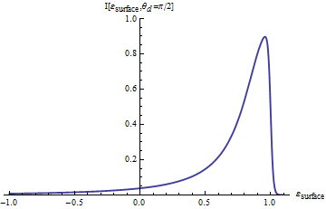
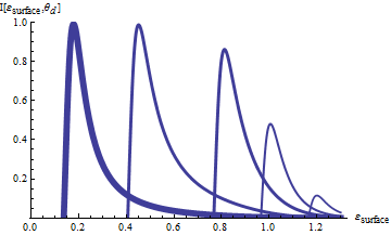
Using the formula I t ^ ( 2 ) β ( Q β , Ο β 0 ) subscript superscript πΌ 2 ^ π‘ β β π π
0 I^{(2)}_{\hat{t}}(\vec{Q},\omega\rightarrow 0) we plot the intensity as a function of the surface electron energy Ο΅ β ( k β ) italic-Ο΅ β π \epsilon(\vec{k}) for different values of the outgoing momentum which is determined by the angle ΞΈ d subscript π π \theta_{d} . We use the chemical potential ΞΌ = 0.3 β e β v . π 0.3 π π£ \mu=0.3ev. binding- work function V 0 β 5 β e β v subscript π 0 5 π π£ V_{0}\approx 5ev and laser energy β β Ξ© β 5 β e β v . Planck-constant-over-2-pi Ξ© 5 π π£ \hbar\Omega\approx 5ev. . The energy of the emitted electrons can be obtained from the fact that the surface momentum k β = q | | = | Q β | β s β i β n β [ ΞΈ d ] \vec{k}=q_{||}=|\vec{Q}|\ sin[\theta_{d}] and the z π§ z component q z = | Q β | β cos β‘ [ ΞΈ d ] subscript π π§ β π subscript π π q_{z}=|\vec{Q}|\cos[\theta_{d}] . If Ο΅ italic-Ο΅ \epsilon is the surface electron energy the free electron energy is given by E f β ( q β , q z ) = β 2 β Q 2 2 β m + V 0 β‘ [ Ο΅ sin β‘ [ ΞΈ d ] ] 2 2 β m + V 0 subscript πΈ π β π subscript π π§ superscript Planck-constant-over-2-pi 2 superscript π 2 2 π subscript π 0 superscript delimited-[] italic-Ο΅ subscript π π 2 2 π subscript π 0 E_{f}(\vec{q},q_{z})=\frac{\hbar^{2}Q^{2}}{2m}+V_{0}\equiv\frac{[\frac{\epsilon}{\sin[\theta_{d}]}]^{2}}{2m}+V_{0} .
The intensity I t ^ ( 2 ) β ( Q β , Ο β 0 ) subscript superscript πΌ 2 ^ π‘ β β π π
0 I^{(2)}_{\hat{t}}(\vec{Q},\omega\rightarrow 0) as a function of surface electrons energy Ο΅ italic-Ο΅ \epsilon for a fixed angle ΞΈ d = Ο 2 subscript π π π 2 \theta_{d}=\frac{\pi}{2} in figure 1 1 1 . In figure 2 2 2 we tune laser frequency and the binding-work function to be 5 . e β v . formulae-sequence 5 π π£ 5.ev. . The plots are for diferent detector angles ΞΈ d subscript π π \theta_{d} .
Figure 1: The intensity I t ^ ( 2 ) β ( Q β , Ο β 0 ) subscript superscript πΌ 2 ^ π‘ β β π π
0 I^{(2)}_{\hat{t}}(\vec{Q},\omega\rightarrow 0) in arbitrary units as a function of surface electrons energy Ο΅ italic-Ο΅ \epsilon for a fixed angle ΞΈ d = Ο 2 subscript π π π 2 \theta_{d}=\frac{\pi}{2} .
Figure 2: The intensity I t ^ ( 2 ) β ( Q β , Ο β 0 ) subscript superscript πΌ 2 ^ π‘ β β π π
0 I^{(2)}_{\hat{t}}(\vec{Q},\omega\rightarrow 0) in arbitrary units as a function of surface electrons energy Ο΅ italic-Ο΅ \epsilon for different detector angle ΞΈ d subscript π π \theta_{d} . Laser frequency and the binding-work function have been chosen to be 5 β e β v . 5 π π£ 5ev. We plot the intensity for ΞΈ d = 0.87 subscript π π 0.87 \theta_{d}=0.87 (the smallest peak) and ΞΈ d = 0.27 subscript π π 0.27 \theta_{d}=0.27 corresponds to the peak around Ο΅ = 0.2 italic-Ο΅ 0.2 \epsilon=0.2 . The values of ΞΈ d subscript π π \theta_{d} considered are ΞΈ d = 0.87 ; 0.77 ; 0.67 ; 0.47 ; 0.27 subscript π π 0.87 0.77 0.67 0.47 0.27
\theta_{d}=0.87;0.77;0.67;0.47;0.27 . The surface energies Ο΅ italic-Ο΅ \epsilon are normalized in units of 0.3 e β v . π π£ ev. , the bottom of the surface conduction band is at Ο΅ = 0 italic-Ο΅ 0 \epsilon=0 . (1 corresponds to0.3 . 0.3 0.3. )
b-The polarization of the emitted electrons
In order to evaluate the polarization of the photoelectrons we need to use the explicit form of the photon polarization vectors e β s β ( ΞΈ , Ο ) subscript β π π π italic-Ο \vec{e}_{s}(\theta,\phi) ,s = 1 , 2 π 1 2
s=1,2 .
In addition we need the photon matrix elements W x β ( k β ) superscript π π₯ β π W^{x}(\vec{k}) , W y β ( k β ) superscript π π¦ β π W^{y}(\vec{k}) and the polarization of the surface electrons < Ο x > expectation superscript π π₯ <\sigma^{x}> ,< Ο y > expectation superscript π π¦ <\sigma^{y}> .
W x β ( k β ) = cos β‘ [ Ο β ( k β ) ] ; W y β ( k β ) = β sin β‘ [ Ο β ( k β ) ] ; < Ο x > = sin β‘ [ Ο β ( k β ) ] ; < Ο y > = β cos β‘ [ Ο β ( k β ) ] ; < Ο z > = 0 formulae-sequence subscript π π₯ β π π β π formulae-sequence subscript π π¦ β π π β π formulae-sequence expectation superscript π π₯ π β π formulae-sequence expectation superscript π π¦ π β π expectation superscript π π§ 0 W_{x}(\vec{k})=\cos[\chi(\vec{k})];W_{y}(\vec{k})=-\sin[\chi(\vec{k})];\hskip 7.22743pt<\sigma^{x}>=\sin[\chi(\vec{k})];<\sigma^{y}>=-\cos[\chi(\vec{k})];<\sigma^{z}>=0
(12)
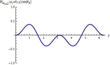
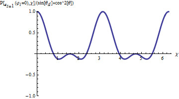
Next we consider the case that the detector is oriented in the t ^ β β ^ π‘ \vec{\hat{t}} direction.
The polarization in the t ^ β β ^ π‘ \vec{\hat{t}} direction is given by :
t ^ β β
< Ο β > = sin β‘ [ ΞΈ d ] β cos β‘ [ Ο β ( k β ) + Ο d ] = sin β‘ [ ΞΈ d ] β cos β‘ [ 2 β Ο β ( k β ) ] = cos β‘ [ ΞΈ d ] β cos β‘ [ 2 β Ο d ] β
β ^ π‘ expectation β π subscript π π π β π subscript italic-Ο π subscript π π 2 π β π subscript π π 2 subscript italic-Ο π \vec{\hat{t}}\cdot<\vec{\sigma}>=\sin[\theta_{d}]\cos[\chi(\vec{k})+\phi_{d}]=\sin[\theta_{d}]\cos[2\chi(\vec{k})]=\cos[\theta_{d}]\cos[2\phi_{d}]
(13)
Therefore the surface polarization electrons will be given by:
P T . S . S . = t ^ β β
< Ο β > = sin β‘ [ ΞΈ d ] β cos β‘ [ Ο β ( k β ) ] subscript π formulae-sequence π π π
β
β ^ π‘ expectation β π subscript π π π β π P_{T.S.S.}=\vec{\hat{t}}\cdot<\vec{\sigma}>=\sin[\theta_{d}]\cos[\chi(\vec{k})] .
For the incoming photons polarization e β s = 2 β ( ΞΈ , Ο ) subscript β π π 2 π italic-Ο \vec{e}_{s=2}(\theta,\phi) we obtain the photoelectrons polarization P ( 2 ) β [ Ο β ( k β ) = Ο d , e β s = 2 β ( ΞΈ = 0 , Ο ) , ΞΈ d , Ο d ] superscript π 2 delimited-[] π β π subscript italic-Ο π subscript β π π 2 π 0 italic-Ο
subscript π π subscript italic-Ο π
P^{(2)}[\chi(\vec{k})=\phi_{d},\vec{e}_{s=2}(\theta=0,\phi),\theta_{d},\phi_{d}] :
P ( 2 ) β [ Ο β ( k β ) = Ο d , e β s = 2 β ( ΞΈ = 0 , Ο ) , ΞΈ d , Ο d ] = sin β‘ [ ΞΈ d ] β cos β‘ [ Ο β ( k β ) + Ο d ] β sin 2 β‘ [ Ο + Ο β ( k β ) ] = superscript π 2 delimited-[] π β π subscript italic-Ο π subscript β π π 2 π 0 italic-Ο
subscript π π subscript italic-Ο π
subscript π π π β π subscript italic-Ο π superscript 2 italic-Ο π β π absent \displaystyle P^{(2)}[\chi(\vec{k})=\phi_{d},\vec{e}_{s=2}(\theta=0,\phi),\theta_{d},\phi_{d}]=\sin[\theta_{d}]\cos[\chi(\vec{k})+\phi_{d}]\sin^{2}[\phi+\chi(\vec{k})]=
sin β‘ [ ΞΈ d ] β cos β‘ [ 2 β Ο β ( k β ) ] β sin 2 β‘ [ Ο + Ο β ( k β ) ] subscript π π 2 π β π superscript 2 italic-Ο π β π \displaystyle\sin[\theta_{d}]\cos[2\chi(\vec{k})]\sin^{2}[\phi+\chi(\vec{k})]
P ( 2 ) β [ Ο β ( k β ) = Ο d , e β s = 2 β ( ΞΈ = 0 , Ο = 0 ) , ΞΈ d , Ο d ] = sin β‘ [ ΞΈ d ] β cos β‘ [ 2 β Ο β ( k β ) ] β sin 2 β‘ [ Ο β ( k β ) ] superscript π 2 delimited-[] π β π subscript italic-Ο π subscript β π π 2 formulae-sequence π 0 italic-Ο 0 subscript π π subscript italic-Ο π
subscript π π 2 π β π superscript 2 π β π \displaystyle P^{(2)}[\chi(\vec{k})=\phi_{d},\vec{e}_{s=2}(\theta=0,\phi=0),\theta_{d},\phi_{d}]=\sin[\theta_{d}]\cos[2\chi(\vec{k})]\sin^{2}[\chi(\vec{k})]
The polarization operator P ( 2 ) superscript π 2 P^{(2)} for the photon polarization e β s = 1 β ( ΞΈ , Ο ) subscript β π π 1 π italic-Ο \vec{e}_{s=1}(\theta,\phi) is given by:
P ( 2 ) β [ Ο β ( k β ) = Ο d , e β s = 1 β ( ΞΈ , Ο ) , ΞΈ d , Ο d ] = sin β‘ [ ΞΈ d ] β cos β‘ [ Ο β ( k β ) + Ο d ] β cos 2 β‘ [ ΞΈ ] β cos 2 β‘ [ Ο β ( k β ) + Ο ] superscript π 2 delimited-[] π β π subscript italic-Ο π subscript β π π 1 π italic-Ο subscript π π subscript italic-Ο π
subscript π π π β π subscript italic-Ο π superscript 2 π superscript 2 π β π italic-Ο \displaystyle P^{(2)}[\chi(\vec{k})=\phi_{d},\vec{e}_{s=1}(\theta,\phi),\theta_{d},\phi_{d}]=\sin[\theta_{d}]\cos[\chi(\vec{k})+\phi_{d}]\cos^{2}[\theta]\cos^{2}[\chi(\vec{k})+\phi]
= sin β‘ [ ΞΈ d ] β cos 2 β‘ [ ΞΈ ] β cos β‘ [ 2 β Ο β ( k β ) ] β cos 2 β‘ [ Ο β ( k β ) + Ο ] absent subscript π π superscript 2 π 2 π β π superscript 2 π β π italic-Ο \displaystyle=\sin[\theta_{d}]\cos^{2}[\theta]\cos[2\chi(\vec{k})]\cos^{2}[\chi(\vec{k})+\phi]
P ( 2 ) β [ Ο β ( k β ) = Ο d , e β s = 1 β ( ΞΈ , Ο = 0 ) , ΞΈ d , Ο d ] = sin β‘ [ ΞΈ d ] β cos 2 β‘ [ ΞΈ ] β cos β‘ [ 2 β Ο β ( k β ) ] β cos 2 β‘ [ Ο β ( k β ) ] superscript π 2 delimited-[] π β π subscript italic-Ο π subscript β π π 1 π italic-Ο
0 subscript π π subscript italic-Ο π
subscript π π superscript 2 π 2 π β π superscript 2 π β π \displaystyle P^{(2)}[\chi(\vec{k})=\phi_{d},\vec{e}_{s=1}(\theta,\phi=0),\theta_{d},\phi_{d}]=\sin[\theta_{d}]\cos^{2}[\theta]\cos[2\chi(\vec{k})]\cos^{2}[\chi(\vec{k})]
We observe that for th surface polarization electrons electrons given by cos β‘ [ Ο β ( k β ) ] π β π \cos[\chi(\vec{k})]
the measured photoelectrons have a polarization
proportional to sin 2 β‘ [ Ο β ( k β ) ] superscript 2 π β π \sin^{2}[\chi(\vec{k})] for photons given by the polarization e β s = 2 β ( ΞΈ = 0 , Ο = 0 ) subscript β π π 2 formulae-sequence π 0 italic-Ο 0 \vec{e}_{s=2}(\theta=0,\phi=0) and cos 2 β‘ [ Ο β ( k β ) ] superscript 2 π β π \cos^{2}[\chi(\vec{k})] for e β s = 2 β ( ΞΈ , Ο = 0 ) subscript β π π 2 π italic-Ο
0 \vec{e}_{s=2}(\theta,\phi=0) .
The two polarizations are shown in figures 2 2 2 and 3 3 3 .
To conclude a model for computing the photoelectrons intensity and polarization has been introduced. We show that the polarization of the photoelectrons depends on the laser polarization.
Figure 3: The photoelectrons polarization P ( 2 ) β [ Ο β ( k β ) = Ο d , e β s = 2 β ( ΞΈ = 0 , Ο = 0 ) , ΞΈ d , Ο d ] superscript π 2 delimited-[] π β π subscript italic-Ο π subscript β π π 2 formulae-sequence π 0 italic-Ο 0 subscript π π subscript italic-Ο π
P^{(2)}[\chi(\vec{k})=\phi_{d},\vec{e}_{s=2}(\theta=0,\phi=0),\theta_{d},\phi_{d}] for the photon polarization e β s = 2 β ( ΞΈ = 0 , Ο = 0 ) subscript β π π 2 formulae-sequence π 0 italic-Ο 0 \vec{e}_{s=2}(\theta=0,\phi=0) as a function the surface electron polar angle Ο β ( k β ) = Ο d π β π subscript italic-Ο π \chi(\vec{k})=\phi_{d} .
Figure 4: The photoelectrons polarization P ( 2 ) β [ Ο β ( k β ) = Ο d , e β s = 1 β ( ΞΈ , Ο = 0 ) , ΞΈ d , Ο d ] superscript π 2 delimited-[] π β π subscript italic-Ο π subscript β π π 1 π italic-Ο
0 subscript π π subscript italic-Ο π
P^{(2)}[\chi(\vec{k})=\phi_{d},\vec{e}_{s=1}(\theta,\phi=0),\theta_{d},\phi_{d}] for the polarization photon e β s = 1 β ( ΞΈ , Ο = 0 ) subscript β π π 1 π italic-Ο
0 \vec{e}_{s=1}(\theta,\phi=0) as a function the surface electron polar angle Ο β ( k β ) = Ο d π β π subscript italic-Ο π \chi(\vec{k})=\phi_{d}
References
(1)
Chris Jozwiak , Cheol-Hwan Park ,Keneth Gotlieb, Choongyu Hwang, Dung-Hai Lee , Steven G.Louie, Jonathan D. Denlinger , Costel R. Rotundu, Robert J. Birgeneau ,Zahid Hussainand Ale Lanzara, Nature Physics 293, vol 9 May (2013).
(2)
Oleg V.Yazyev ,Joel Moore, and Steven G.Louie, Phys.Rev.Lett 105 , 266806(2010).
(3)
Phys.Rev.Lett 109 , 097601(2012)
Cheo-Hwan Park and Steven G.Louie , Phys.Rev.Lett 109 , 097601(2012)
(4)
Y.H.Wang ,D.Hsieh D.Pilon ,L.Fu, D.R. Gardner ,Y.S. :ee and N.Gedik. Phys.Rev.Lett 107 , 207602(2011)
(5)
Fan Zhang,C.L. Kane, and E.J. Mele ,Phys. Rev.B 86 ,081303(R)(2012)
(6)
Liang Fu , Phys.Rev.Lett 103 ,266801 (2009).
(7)
C.L.Kane and E.J. Mele Phys.Rev.Lett.75 ,146802(2005)
(8)
B.A,Volkov and O.A.Pankratov Jetp Lett. 61 2015 (1988)
(9)
Xiao-Liang Qi and Shou-Cheng-Zhang Rev.Of Modern Physics 83 1057(2011)
(10)
D.Schmeltzer, Advances in Condensed Matter and Material Research Editors Hans Geelvinck and Sjaak Reyst volume 10 chapter 9 9 9 , pages 379 β 403 379 403 379-403 (2011).
(11)
D.Schmeltzer and Avadh Saxena, Phys.Rev.B 88 035140(20013).
(12)
S.Donaich and E.H. Sondheimer ββGreenβs Functions for Solid State Physicistsββ Imperial College Press (1988)
(13)
Lin Miao, Z.F.Wang, Wenmei Ming, Meng-Yu Yao ,Meixiano Wang, Fang Yang, Y.R. Song, Fengfeng Zhu, Alexei V. Fedorov, Z.Sun, C.L. Gao, Canhua Liu, Qi-Kun Xue, Chao-Xing Liu, FengLiu, Dong Qian and Jin-Feng Jia, PNAS ,2758-2762 ,vol 110 no.8 (2013).