Perturbatively improving renormalization constants

Abstract:

Renormalization factors relate the observables obtained on the lattice to their measured counterparts in the continuum in a suitable renormalization scheme. They have to be computed very precisely which requires a careful treatment of lattice artifacts. In this work we present a method to suppress these artifacts by subtracting one-loop contributions proportional to the square of the lattice spacing calculated in lattice perturbation theory.

DESY 13 - 190, Edinburgh 2013/25

1 Introduction

Renormalization factors in lattice Quantum Chromodynamics (QCD) relate observables computed on finite lattices to their continuum counterparts in specific renormalization schemes. Therefore, their determination should be as precise as possible in order to allow for a reliable comparison with experimental results. A widely used method to calculate these factors is the so-called Rome-Southampton method [1] (utilizing the RI-MOM scheme). Like (almost) all quantities evaluated in lattice QCD also renormalization factors computed in this non-perturbative scheme suffer from discretization effects. In this paper we describe a method to suppress these lattice artifacts using a subtraction procedure based on perturbation theory. It has been published in Ref. [2] and the reader is referred for all details to this reference.

In a recent paper of the QCDSF/UKQCD collaboration [3] a comprehensive discussion and comparison of perturbative and nonperturbative renormalization have been given. It was shown that a subtraction of the complete lattice artifacts in one-loop lattice perturbation theory improves the results for the Z factors significantly. While being very effective this procedure is rather involved and not suited as a general method for more complex operators, especially for operators with more than one covariant derivative, and complicated lattice actions. An alternative approach can be based on the subtraction of one-loop terms of order $a^{2}$, with $a$ being the lattice spacing. The computation of those terms has been developed by the authors of Ref. [4] and applied to various operators for different actions.

We study the flavor-nonsinglet quark-antiquark operators given in Table 1.

Operator (multiplet)	Notation	Representation	Operator basis
$\bar{u}\,d$	$\mathcal{O}^{S}$	$\tau_{1}^{(1)}$	$\mathcal{O}^{S}$
$\bar{u}\,\gamma_{\mu}\,d$	$\mathcal{O}_{\mu}^{V}$	$\tau_{1}^{(4)}$	$\mathcal{O}_{1}^{V},\mathcal{O}_{2}^{V},\mathcal{O}_{3}^{V},\mathcal{O}_{4}^{V}$
$\bar{u}\,\gamma_{\mu}\gamma_{5}\,d$	$\mathcal{O}_{\mu}^{A}$	$\tau_{4}^{(4)}$	$\mathcal{O}_{1}^{A},\mathcal{O}_{2}^{A},\mathcal{O}_{3}^{A},\mathcal{O}_{4}^{A}$
$\bar{u}\,\sigma_{\mu\nu}\,d$	$\mathcal{O}_{\mu\nu}^{T}$	$\tau_{1}^{(6)}$	$\mathcal{O}_{12}^{T},\mathcal{O}_{13}^{T},\mathcal{O}_{14}^{T},\mathcal{O}_{23}^{T},\mathcal{O}_{24}^{T},\mathcal{O}_{34}^{T}$
$\bar{u}\,\gamma_{\mu}\stackrel{{\scriptstyle\leftrightarrow}}{{D_{\nu}}}\,d$	$\mathcal{O}_{\mu\nu}\to\mathcal{O}^{v_{2,a}}$	$\tau_{3}^{(6)}$	$\mathcal{O}_{\{12\}},\mathcal{O}_{\{13\}},\mathcal{O}_{\{14\}},\mathcal{O}_{\{23\}},\mathcal{O}_{\{24\}},\mathcal{O}_{\{34\}}$
$\bar{u}\,\gamma_{\mu}\stackrel{{\scriptstyle\leftrightarrow}}{{D_{\nu}}}\,d$	$\mathcal{O}_{\mu\nu}\to\mathcal{O}^{v_{2,b}}$	$\tau_{1}^{(3)}$	$1/2(\mathcal{O}_{11}+\mathcal{O}_{22}-\mathcal{O}_{33}-\mathcal{O}_{44})$,
			$1/\sqrt{2}(\mathcal{O}_{33}-\mathcal{O}_{44}),1/\sqrt{2}(\mathcal{O}_{11}-\mathcal{O}_{22})$

Table 1: Operators and their representations with respect to the hypercubic group as investigated in the present paper. The symbol $\{...\}$ means total symmetrization. A detailed group theoretical discussion is given in [5].

The corresponding renormalization factors have been measured (and chirally extrapolated) at the lattice coupling $\beta=6/g^{2}=5.20,5.25,5.29$ and $5.40$ using $N_{f}=2$ clover improved Wilson fermions with plaquette gauge action [3]. The Sommer scale $r_{0}$ is taken to be $r_{0}=0.501\,{\rm fm}$ and the relation between the lattice spacing $a$ and $\beta$ is given by $r_{0}/a=6.050\,(\beta=5.20),6.603\,(\beta=5.25),7.004\,(\beta=5.29)$ and $8.285\,(\beta=5.40)$ [6]. This results in the corresponding values $a(\beta)=(0.42,0.39,0.36,0.31){\rm GeV}^{-1}$. All results are computed in Landau gauge. The clover parameter $c_{SW}$ used in the perturbative calculation discussed below is set to its lowest order value $c_{SW}=1$.

2 Renormalization group invariant operators

We define a so-called RGI (renormalization group invariant) operator, which is independent of scale $M$ and scheme $\mathcal{S}$, by [3]

$$\mathcal{O}^{\rm RGI}=\Delta Z^{\mathcal{S}}(M)\,\mathcal{O}^{\mathcal{S}}(M)=Z^{\rm RGI}(a)\,\mathcal{O}_{\rm bare}\,$$ (1)

with

$$\Delta Z^{\mathcal{S}}(M)=\left(2\beta_{0}\frac{g^{\mathcal{S}}(M)^{2}}{16\,\pi^{2}}\right)^{-(\gamma_{0}/2\beta_{0})}\,{\rm exp}\left\{\int_{0}^{g^{\mathcal{S}}(M)}dg^{\prime}\left(\frac{\gamma^{\mathcal{S}}(g^{\prime})}{\beta^{\mathcal{S}}(g^{\prime})}+\frac{\gamma_{0}}{\beta_{0}g^{\prime}}\right)\right\}$$ (2)

and the RGI renormalization constant (depending on the lattice spacing $a$ via the lattice coupling)

$$Z^{\rm RGI}(a)=\Delta Z^{\mathcal{S}}(M)\,\,Z^{\mathcal{S}}_{\rm bare}(M,a)\,.$$ (3)

Here $g^{\mathcal{S}}$, $\gamma^{\mathcal{S}}$ and $\beta^{\mathcal{S}}$ are the coupling constant, the anomalous dimension and the $\beta$-function in scheme $\mathcal{S}$, respectively. Relations (1), (2) and (3) allow us to compute the operator $\mathcal{O}$ in any scheme and at any scale we like, once $Z^{\rm RGI}$ is known. Ideally, $Z^{\rm RGI}$ depends only on the bare lattice coupling, but not on the momentum $p$ which determines the scale via $M^{2}=p^{2}$. Computed on a lattice, however, it suffers from lattice artifacts, e.g., it contains contributions proportional to $a^{2}p^{2}$, $(a^{2}p^{2})^{2}$ etc. For a precise determination it is essential to have these discretization errors under control.

As the ${\rm RI}^{\prime}$-MOM scheme is in general not $O(4)$-covariant even in the continuum limit, it is not very suitable for computing the anomalous dimensions needed in (2). Therefore we use an intermediate scheme $\mathcal{S}$ with known anomalous dimensions and calculate $Z^{\rm RGI}$ as follows:

$$Z^{\rm RGI}(a)=\Delta Z^{\mathcal{S}}(M)\,Z^{\mathcal{S}}_{\rm RI^{\prime}-MOM}(M)\,Z^{\rm RI^{\prime}-MOM}_{\rm bare}(M,a)\,.$$ (4)

It turns out that a type of momentum subtraction scheme is a good choice for $\mathcal{S}$ (for details see Ref. [3]).

3 Subtraction of order $a^{2}$ one-loop lattice artifacts

The diagrammatic approach to compute the one-loop $a^{2}$ terms for the $Z$ factors of local and one-link operators has been developed in Ref. [4]. The general case of Wilson type improved fermions is discussed in [7]. We compute a common $Z$ factor for each multiplet given in Table 1. As examples we give here (up to terms of higher order in the bare coupling $g^{2}$ and $a^{2}$)

$$Z_{S} = 1+\frac{g^{2}\,C_{F}}{16\pi^{2}}\,\Bigg{\{}-23.3099+3\,\log(a^{2}S_{2})$$ (5)

$$+\,a^{2}\left[S_{2}\left(1.64089-\frac{239}{240}\log(a^{2}{S_{2}})\right)+\frac{S_{4}}{S_{2}}\left(1.95104-\frac{101}{120}\log(a^{2}{S_{2}})\right)\right]\Bigg{\}}\,,$$

$$Z_{v_{2,a}} = 1+\frac{g^{2}\,C_{F}}{16\pi^{2}}\,\Bigg{\{}6.93831-\frac{8}{3}\log(a^{2}S_{2})-\frac{2}{9}\frac{S_{4}}{(S_{2})^{2}}$$ (6)

$$+\,{a^{2}}\,\Bigg{[}S_{2}\,\left(-1.50680+\frac{167}{180}\log(a^{2}S_{2})\right)$$

$$\hskip 8.5359pt+\frac{S_{4}}{S_{2}}\,\left(2.63125-\frac{197}{180}\log(a^{2}S_{2})\right)-\frac{71}{540}\frac{{S_{4}}^{2}}{(S_{2})^{3}}-\frac{82}{135}\frac{S_{6}}{(S_{2})^{2}}\Bigg{]}\Bigg{\}}\,,$$

where we have introduced the notations $S_{n}=\sum_{\lambda=1}^{4}\,p_{\lambda}^{n}$ ($p_{\lambda}$ being the momentum components) and $C_{F}=4/3$. The $Z$ factors are written generically as

$$Z=1+\frac{g^{2}\,C_{F}}{16\pi^{2}}\,Z_{\rm 1-loop}(p,a)+{a^{2}}g^{2}Z^{(a^{2})}_{\rm 1-loop}(p,a)\,.$$ (7)

We emphasize that the numerical coefficients in the above expressions are either exact rationals or can be computed to a very high precision.

Now we turn to the subtraction procedure applied to the Monte Carlo data $Z^{\rm RI^{\prime}-MOM}_{\rm bare}(p,a)_{\rm MC}$. The subtraction of order $a^{2}$ terms is not unique - we have different possibilities. The only restriction is that in one-loop perturbation theory they should agree. We investigate the following definitions (choices (s) and (m)) of subtracted renormalization constants,

$$Z^{\rm RI^{\prime}-MOM}_{\rm bare}(p,a)_{\rm MC,sub,s} = Z^{\rm RI^{\prime}-MOM}_{\rm bare}(p,a)_{\rm MC}-{a^{2}}\,g_{\star}^{2}\,Z^{(a^{2})}_{\rm 1-loop}(p,a)\,,$$ (8)

$$Z^{\rm RI^{\prime}-MOM}_{\rm bare}(p,a)_{\rm MC,sub,m} = Z^{\rm RI^{\prime}-MOM}_{\rm bare}(p,a)_{\rm MC}\,\times\left(1-{a^{2}}\,g_{\star}^{2}\,Z^{(a^{2})}_{\rm 1-loop}(p,a)\right)\,,$$ (9)

where $g_{\star}^{2}$ can be chosen to be either $g^{2}$ or the boosted coupling $g_{\rm B}^{2}=g^{2}/P(g)=g^{2}+O(g^{4})$, $P(g)$ being the measured plaquette at $\beta=6/g^{2}$. The effect of the different subtractions is shown in Fig. 1.

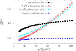
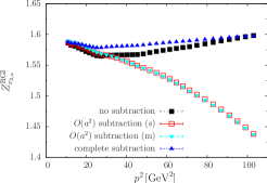
Figure 1: Unsubtracted and subtracted renormalization constants for the scalar operator $\mathcal{O}^{S}$ (left) and the one-link operator $\mathcal{O}^{v_{2,a}}$ (right) at $\beta=5.40$, for $p^{2}\gtrsim 10\,{\rm GeV}^{2}$ and $r_{0}\,\Lambda_{\rm\overline{MS}}=0.700$. The $a^{2}$ subtractions are of type (s) and (m) with $g_{\star}=g_{\rm B}$.

The complete one-loop subtraction leads to almost flat $Z^{\rm RGI}$, whereas the Z factors obtained from the one-loop $a^{2}$ subtractions show a significant dependence on $p^{2}$ which has to be taken into account in the calculation.

We expect that $Z^{\rm RI^{\prime}-MOM}_{\rm bare}(p,a)_{\rm MC,sub}$ contains terms proportional to $a^{2n}$ ($n\geq 2$) even at order $g^{2}$, as well as the lattice artifacts from higher orders in perturbation theory, constrained only by hypercubic symmetry. Therefore, we parametrize the subtracted data for each $\beta$ in terms of the hypercubic invariants $S_{n}$ as follows

$$Z^{\mathcal{S}}_{\rm RI^{\prime}-MOM}(p)\, Z^{\rm RI^{\prime}-MOM}_{\rm bare}(p,a)_{\rm MC,sub}=\frac{Z^{\rm RGI}(a)}{\Delta Z^{\mathcal{S}}(p)\,\left[1+b_{1}\,(g^{\mathcal{S}})^{8}\right]}+$$

$$a^{2}\left(c_{1}\,S_{2}+c_{2}\,\frac{S_{4}}{S_{2}}+c_{3}\,\frac{S_{6}}{(S_{2})^{2}}\right)+a^{4}\,\left(c_{4}\,(S_{2})^{2}+c_{5}\,S_{4}\right)+a^{6}\left(c_{6}\,(S_{2})^{3}+c_{7}\,S_{4}\,S_{2}+c_{8}\,S_{6}\right)\,.$$

The parameter $b_{1}$ is introduced to compensate for the truncation errors in the expressions from continuum perturbation theory. There are also further non-polynomial invariants at order $a^{4},a^{6}$, but their behavior is expected to be well described by the invariants which have been included already.

Together with the target parameter $Z^{\rm RGI}(a)$ we have ten parameters for this general case. In view of the limited number of data points for each single $\beta$ value $(5.20$, $5.25$, $5.29$, $5.40)$ we apply the ansatz (3) at several $\beta$ values simultaneously, assuming $\beta$-independent fit parameters $b_{1}$ and $c_{i}$. The renormalization factors are influenced by the choice for $r_{0}\,\Lambda_{\rm\overline{MS}}$. This quantity enters $\Delta Z^{\mathcal{S}}(M)$ in (2) via the corresponding coupling $g^{\mathcal{S}}(M)$ (for details see [3]). We choose $r_{0}\,\Lambda_{\rm\overline{MS}}=0.700$ [8] and $0.789$ [9] in order to test the influence of $r_{0}\,\Lambda_{\rm\overline{MS}}$.

The fit procedure as sketched above has quite a few degrees of freedom and it is essential to investigate their influence carefully. A criterion for the choice of the minimal value of $p^{2}$ is provided by the breakdown of perturbation theory at small momenta. The data suggest [3] that we are on the ’safe side’ when choosing $p^{2}_{\min}=10\,\mbox{GeV}^{2}$. As the upper end of the fit interval we take the maximal available momentum at given coupling $\beta$.

Other important factors are

• Type of subtraction: As discussed above, the procedure of the one-loop subtraction is not unique. We consider the two choices (s) and (m) with either bare $g$ or boosted coupling $g_{B}$.

• Selection of hypercubic invariants: For the quality of the fit it is essential to have an appropriate description of the lattice artifacts which remain after subtraction. This is connected to the question whether the $a^{2}$ subtraction has been sufficient to subtract (almost) all $a^{2}$ artifacts. Therefore, we perform fits with various combinations of structures in (3). One should mention that the concrete optimal (i.e. minimal) set of $c_{i}$ depends strongly on the momenta of the available Monte Carlo data - momenta close to the diagonal in the Brillouin zone require fewer structures to be fitted than far off-diagonal ones.

As discussed in detail in [2] we are not able to find one combination of the investigated subtraction types and parameter sets $\{c_{i}\}$ which is superior to all others. This is partly due to the fact that the available data set is almost diagonal in the momentum components. Therefore, we rely on our experience, which suggests, e.g., the use of the boosted coupling $g_{B}$ in the subtraction prodecure. One further important consideration is the comparison with the results based on the complete one-loop subtraction which serve as benchmarks. In the end, we favor the simple subtraction (s) with boosted coupling $g_{B}$ using all parameters $c_{i}$ in the ansatz (3).

In Fig. 2 we show as examples the corresponding results for the operators $\mathcal{O}^{S}$ and $\mathcal{O}^{v_{2,a}}$ compared to the results obtained by the complete one-loop subtraction.

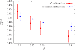
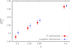
Figure 2: $Z_{S}^{\rm RGI}$ (left) and $Z_{v_{2,a}}^{\rm RGI}$ (right) at $r_{0}\,\Lambda_{\rm\overline{MS}}=0.700$ as a function of $\beta$ using all $c_{i}$ compared to the complete one-loop subtraction.

The final renormalization factors are collected in Table 2

Op.	$r_{0}\,\Lambda_{\rm\overline{MS}}$	$Z^{\rm RGI}|_{\beta=5.20}$	$Z^{\rm RGI}|_{\beta=5.25}$	$Z^{\rm RGI}|_{\beta=5.29}$	$Z^{\rm RGI}|_{\beta=5.40}$
$\mathcal{O}^{S}$	$0.700$	$0.4530(34)$	$0.4475(33)$	$0.4451(32)$	$0.4414(30)$
	$0.789$	$0.4717(44)$	$0.4661(65)$	$0.4632(54)$	$0.4585(27)$
$\mathcal{O}^{V}$	$0.700$	$0.7163(26)$	$0.7253(26)$	$0.7308(25)$	$0.7451(24)$
	$0.789$	$0.7238(72)$	$0.7319(94)$	$0.7365(99)$	$0.7519(50)$
$\mathcal{O}^{A}$	$0.700$	$0.7460(41)$	$0.7543(40)$	$0.7590(39)$	$0.7731(37)$
	$0.789$	$0.7585(46)$	$0.7634(77)$	$0.7666(81)$	$0.7805(30)$
$\mathcal{O}^{T}$	$0.700$	$0.8906(43)$	$0.9036(42)$	$0.9108(41)$	$0.9319(39)$
	$0.789$	$0.8946(85)$	$0.9041(111)$	$0.9075(120)$	$0.9316(49)$
$\mathcal{O}^{v_{2,a}}$	$0.700$	$1.4914(55)$	$1.5131(55)$	$1.5266(54)$	$1.5660(53)$
	$0.789$	$1.4635(108)$	$1.4776(112)$	$1.4926(90)$	$1.5397(58)$
$\mathcal{O}^{v_{2,b}}$	$0.700$	$1.5061(37)$	$1.5218(37)$	$1.5329(36)$	$1.5534(35)$
	$0.789$	$1.4601(151)$	$1.4727(206)$	$1.4863(165)$	$1.5115(140)$

Table 2: $Z^{\rm RGI}$ values using the subtraction (s) with $g_{B}$. The errors are obtained from the nonlinear fit procedure.

using the two different $r_{0}\,\Lambda_{\rm\overline{MS}}$ values $0.700$ and $0.789$. This shows the influence of the choice of $r_{0}\,\Lambda_{\rm\overline{MS}}$ (depending on the anomalous dimension of the operator). For the investigated operators and $\beta$ values we find for the relative differences of the $Z^{\rm RGI}$

$$\delta Z^{\rm RGI}=\Bigg{|}\frac{Z^{\rm RGI}_{r_{0}\,\Lambda_{\rm\overline{MS}}=0.700}-Z^{\rm RGI}_{r_{0}\,\Lambda_{\rm\overline{MS}}=0.789}}{Z^{\rm RGI}_{r_{0}\,\Lambda_{\rm\overline{MS}}=0.700}}\Bigg{|}\lesssim 0.04\,.$$ (11)

The $Z$ factors of the local (one-link) operators differ with $1\,\%$ ($2\,\%$) from the corresponding results obtained via the complete one-loop subtraction.

From the present investigation we conclude: The alternatively proposed ’reduced’ subtraction algorithm can be used for the determination of the renormalization factors if the complete subtraction method is not available. Possible applications could be $Z$ factors for $N_{f}=2+1$ calculations with more complicated fermionic and gauge actions where one-loop results to order $a^{2}$ are available (for the fermionic SLiNC action with improved Symanzik gauge action see Ref. [10]).

References

• [1] G. Martinelli, C. Pittori, C. T. Sachrajda, M. Testa and A. Vladikas, Nucl. Phys. B 445 (1995) 81 [arXiv:hep-lat/9411010].
• [2] M. Constantinou, M. Costa, M. Göckeler, R. Horsley, H. Panagopoulos, H. Perlt, P. E. L. Rakow, G. Schierholz and A. Schiller, Phys. Rev.  D 87 (2013) 096019 [arXiv:1303.6776[hep-lat]].
• [3] M. Göckeler, R. Horsley, Y. Nakamura, H. Perlt, D. Pleiter, P. E. L. Rakow, A. Schäfer, G. Schierholz, A. Schiller, H. Stüben and J. M. Zanotti, (QCDSF/UKQCD Collaborations), Phys. Rev. D 82 (2010) 114511 [Erratum-ibid. D 86 (2012) 099903] [arXiv:1003.5756[hep-lat]].
• [4] M. Constantinou, V. Lubicz, H. Panagopoulos and F. Stylianou, JHEP 0910 (2009) 064 [arXiv:0907.0381[hep-lat]].
• [5] M. Göckeler, R. Horsley, E.-M. Ilgenfritz, H. Perlt, P. E. L. Rakow, G. Schierholz and A. Schiller, Phys. Rev. D 54 (1996) 5705 [arXiv:hep-lat/9602029].
• [6] G. S. Bali, P. C. Bruns, S. Collins, M. Deka, B. Gläßle, M. Göckeler, L. Greil, T.R. Hemmert, R. Horsley, J. Najjar, Y. Nakamura, A. Nobile, D. Pleiter, P. E. L. Rakow, A. Schäfer, R. Schiel, G. Schierholz, A. Sternbeck and J. M. Zanotti (QCDSF Collaboration), Nucl. Phys. B 866 (2013) 1 [arXiv:1206.7034[hep-lat]].
• [7] C. Alexandrou, M. Constantinou, T. Korzec, H. Panagopoulos and F. Stylianou, Phys. Rev. D 86 (2012) 014505 [arXiv:1201.5025[hep-lat]].
• [8] QCDSF collaboration, in preparation.
• [9] P. Fritzsch, F. Knechtli, B. Leder, M. Marinkovic, S. Schaefer, R. Sommer and F. Virotta (ALPHA Collaboration), Nucl. Phys. B 865 (2012) 397 [arXiv:1205.5380[hep-lat]].
• [10] A. Skouroupathis and H. Panagopoulos, PoS LATTICE 2010, 240 (2010).